Two-dimensional defect modes in optically induced photonic lattices

Abstract

In this article, localized linear defect modes due to bandgap guidance in two-dimensional photonic lattices with localized or non-localized defects are investigated theoretically. First, when the defect is localized and weak, eigenvalues of defect modes bifurcated from edges of Bloch bands are derived analytically. It is shown that in an attractive (repulsive) defect, defect modes bifurcate out from Bloch-band edges with normal (anomalous) diffraction coefficients. Furthermore, distances between defect-mode eigenvalues and Bloch-band edges are exponentially small functions of the defect strength, which is very different from the one-dimensional case where such distances are quadratically small with the defect strength. It is also found that some defect-mode branches bifurcate not from Bloch-band edges, but from quasi-edge points within Bloch bands, which is very unusual. Second, when the defect is localized but strong, defect modes are determined numerically. It is shown that both the repulsive and attractive defects can support various types of defect modes such as fundamental, dipole, quadrupole, and vortex modes. These modes reside in various bandgaps of the photonic lattice. As the defect strength increases, defect modes move from lower bandgaps to higher ones when the defect is repulsive, but remain within each bandgap when the defect is attractive, similar to the one-dimensional case. The same phenomena are observed when the defect is held fixed while the applied dc field (which controls the lattice potential) increases. Lastly, if the defect is non-localized (i.e. it persists at large distances in the lattice), it is shown that defect modes can be embedded inside the continuous spectrum, and they can bifurcate out from edges of the continuous spectrum algebraically rather than exponentially.

I Introduction

Study of light propagation in periodic media such as photonic crystals and optically induced photonic lattices is of great interest to both fundamental physics and applications Russell ; Joannopoulos ; Christodoulides_review ; Kivshar_book . It is well known that the unique feature of such periodic systems is the existence of bandgap structures in its linear spectrum. Inside the bands, eigenmodes of its spectrum are Bloch waves, while inside bandgaps, wave propagation is forbidden because of the repeated Bragg reflections. To guide light in periodic media, one of the convenient ways is to introduce a defect into the medium. The defect can support linear localized modes (called defect modes) inside bandgaps of the periodic medium. Such modes could only propagate along the defect direction (their propagation along other directions is forbidden for being inside bandgaps), thus defect guidance (or bandgap guidance) of light is realized.

Defects and the corresponding defect modes (DMs) have been widely investigated in the field of photonic crystals Russell ; Joannopoulos , where bandgaps and defect modes are in the temporal frequency domains. Recently, reconfigurable optically induced photonic lattices in photorefractive crystals with and without defects were successfully generated Segev_nature ; ChenPRL04 ; ChenYangPRL ; Chen_OE . In photonic lattices, bandgaps are in the spatial frequency domains. Linear DMs in one-dimensional (1D) photonic lattices have been analyzed both theoretically and experimentally in YangOL ; YangChendefect ; Chen_OE . Nonlinear defect solitons in 1D photonic lattices have also been theoretically explored Kivshar_defect ; YangChenPRE (see also a study of DMs and defect solitons in 1D waveguide arrays in Silberberg ). A more interesting subject is DMs in 2D photonic lattices, where richer light-guiding possibilities can arise. Recently, we have observed that a localized defect in 2D lattices can guide not only fundamental modes, but also higher-order modes with delicate tail structures ChenYangPRL . However, our theoretical understanding on such new types of 2D DM structures is still far from satisfactory. For instance, it is still unclear what types of DMs a 2D defect can possibly support, and how localized these DMs can be in defects of various depths. We should mention that in uniformly periodic photonic lattices, a number of nonlinear localized modes such as fundamental, dipole, vortex, dipole-array and vortex-array solitons have been reported Eisenberg98 ; Segev_nature ; ChenPRL04 ; Neshev_dipole ; Yang_dipole ; Yang_Muss ; Chen_vortex ; Segev_vortex ; Segev_highervortex ; Kivshar_C_onemode ; Shi . Solitons in Bessel-ring lattices and 2D quasi-periodic lattices have been reported as well Kartashov ; Chen_ring ; Ablowitz . These nonlinear modes may be regarded as linear DMs of the defect induced by solitons themselves. Hence studies of linear DMs in defective lattices and nonlinear solitons in uniform lattices can stimulate each other. Indeed, many types of linear DMs we will report in this paper do resemble certain types of strongly localized solitons in 2D uniform lattices (see Segev_highervortex ; Kivshar_C_onemode ; Shi ). However, many differences exist between solitons in uniform lattices and linear DMs in defective lattices. For instance, low-amplitude solitons in uniform lattices are very broad and occupy many lattice sites, thus the “defects” these solitons generate are very different from the single-site defects as created in the experiments of ChenYangPRL and considered in several sections of this paper. Another difference is that, in uniform lattices, centers of solitons can be located at two positions (on-site and off-site) in the 1D case Peli_1D and four positions at or between lattice sites in the 2D case Shi . However, in defective lattices, linear DMs can only be centered at the defect site. Due to these differences, previous results on solitons in uniform lattices can not be naively copied over to linear DMs.

In this article, linear localized DMs in 2D optically induced photonic lattices with localized or non-localized defects are systematically studied theoretically. For localized defects, we show numerically that both the attractive and repulsive defects can support various types of 2D DMs such as fundamental, dipole, quadrupole, and vortex modes. These modes reside in various bandgaps of the photonic lattice. When the defect is weak, DMs are further studied analytically by asymptotic methods. We show that in a weak repulsive defect, DMs bifurcate out from Bloch-band edges with anomalous diffraction coefficients. The situation is opposite for attractive defects. We also show that distances between DM eigenvalues and Bloch-band edges are exponentially small functions of the defect strength, which is very different from the 1D case where such dependence is quadratic. In addition, we find that some DM branches bifurcate not from Bloch-band edges, but from quasi-edge points within Bloch bands, which is very unusual. As the defect strength increases, DMs move from lower bandgaps to higher ones when the defect is repulsive, but remain within each bandgap when the defect is attractive. The same phenomena are observed when the defect is held fixed while the applied dc field (which controls the lattice potential) increases. If the defect is non-localized (i.e. it does not disappear at large distances in the lattice), we show that DMs exhibit some new features, such as DMs can be embedded inside the continuous spectrum, and they can bifurcate out from edges of the continuous spectrum algebraically rather than exponentially.

II The Theoretical Model

We begin our study by considering one ordinarily polarized 2D square-lattice beam with a localized defect and one extraordinarily polarized probe beam with very low intensity launched simultaneously into a photorefractive crystal. The two beams are mutually incoherent, and the defective lattice beam is assumed to be uniform along the propagation direction (such defective 2D lattices have been created in our earlier experiments ChenYangPRL ). In this situation, the dimensionless governing equation for the probe beam is Segev_nature ; Christodoulides_model ; Segev_model ; YangChendefect :

$$iU_{z}+U_{xx}+U_{yy}-\frac{E_{0}}{1+I_{L}(x,y)}U=0.$$ (2.1)

Here $U$ is the slowly-varying amplitude of the probe beam, $(x,y)$ are transverse distances (in units of $D/\pi$ with $D$ being the lattice spacing), $z$ is the propagation distance (in units of $2k_{1}D^{2}/\pi^{2}$), $E_{0}$ is the applied dc field (in units of $\pi^{2}/(k_{0}^{2}n_{e}^{4}D^{2}r_{33})$),

$$I_{L}=I_{0}\cos^{2}(x)\cos^{2}(y)[1+\epsilon F_{D}(x,y)]$$ (2.2)

is the intensity function of the photonic lattice (normalized by $I_{d}+I_{b}$, where $I_{d}$ is the dark irradiance of the crystal and $I_{b}$ the background illumination), $I_{0}$ is the peak intensity of the otherwise uniform photonic lattice, $F_{D}(x,y)$ describes the shape of the defect, $\epsilon$ controls the strength of the defect, $k_{0}=2\pi/\lambda_{0}$ is the wave number ($\lambda_{0}$ is the wavelength), $k_{1}=k_{0}n_{e}$, $n_{e}$ is the unperturbed refractive index, and $r_{33}$ is the electro-optic coefficient of the crystal. Notice that the period of the square lattice has been normalized to be $\pi$. For localized defects which we are considering in this section as well as sections III and IV, $F_{D}(x,y)$ is a localized function (the case of non-localized defects will be considered in Sec. V). In our numerical computations, for simplicity, we choose $F_{D}(x,y)$ to be YangChendefect ; ChenYangPRL

$$F_{D}(x,y)=\exp[-(x^{2}+y^{2})^{4}/128],$$ (2.3)

which describes a single-site defect. When $\epsilon>0$, the lattice intensity $I_{L}$ at the defect site is higher than that at the surrounding regions, and a defect like this is called an attractive defect. Otherwise, the defect is called a repulsive one. The defected lattice profiles with $\epsilon=\pm 0.9$ will be displayed later in the text (see Figs. 5 and 7). Throughout this paper (except in section V), we will choose the lattice peak intensity to be $I_{0}=6$.

Localized defect modes in Eq. (2.1) are sought in the form of

$$U(x,y;z)=u(x,y)\exp(-i\mu z),$$ (2.4)

where $\mu$ is the propagation constant, and $u(x,y)$ is a localized function in $x$ and $y$. After substituting the above expression into Eq. (2.1), a linear eigenvalue equation for $u(x,y)$ is derived:

$$u_{xx}+u_{yy}+[\mu-\frac{E_{0}}{1+I_{L}(x,y)}]u=0.$$ (2.5)

In the rest of this paper, we will comprehensively analyze DMs in this 2D Schrödinger equation with defective lattice potentials by both analytical and numerical techniques.

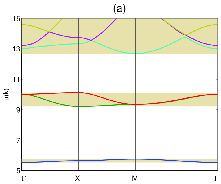
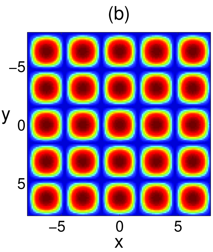
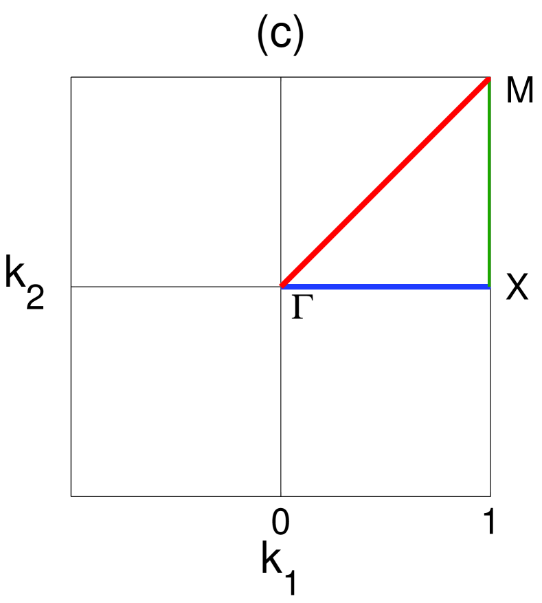
Figure 1: (a) Diffraction relation of the uniform lattice potential (2.8) with $E_{0}=15$ and $I_{0}=6$ in the reduced Brillouin zone along the direction of $\Gamma\rightarrow X\rightarrow M\rightarrow\Gamma$. Shaded: first three Bloch bands. (b) Potential (i.e. effective refractive index change) (2.8) in the $(x,y)$ plane. (c) The first Brillouin zone of the 2D lattice in the reciprocal lattice space.

Before the analysis of DMs, let us first look at the diffraction relation and bandgap structure of Eq. (2.5) without defects (i.e., $\epsilon=0$). According to the Bloch theorem, eigenfunctions of Eq. (2.5) can be sought in the form of

$$u(x,y)=e^{ik_{1}x+ik_{2}y}G(x,y;k_{1},k_{2}),\quad\mu=\mu(k_{1},k_{2}),$$ (2.6)

where $\mu=\mu(k_{1},k_{2})$ is the diffraction relation, wavenumbers $k_{1}$, $k_{2}$ are in the first Brillouin zone, i.e. $-1\leq k_{1},k_{2}\leq 1$, and $G(x,y;k_{1},k_{2})$ is a periodic function in $x$ and $y$ with the same period $\pi$ (in normalized units) as the uniform lattice of (2.2). By substituting the above Bloch solution into Eq. (2.5) (with $\epsilon=0$), we find that the diffraction relation $\mu(k_{1},k_{2})$ of our 2D uniform lattice will be obtained by solving the following eigenvalue problem

$$[(\partial_{x}+ik_{1})^{2}+(\partial_{y}+ik_{2})^{2}+V(x,y)]G(x,y)=-\mu G(x,y)$$ (2.7)

with the uniform periodic potential

$$V(x,y)=-\frac{E_{0}}{1+I_{0}\cos^{2}(x)\cos^{2}(y)}.$$ (2.8)

Figure 1 shows the diffraction relation of Eq. (2.5) along three characteristic high-symmetry directions ($\Gamma\rightarrow X\rightarrow M\rightarrow\Gamma$) of the irreducible Brillouin zone. It can be seen that there exist three complete gaps which are named the semi-infinite, first and second gaps respectively. They correspond to the white areas in Figure 1 from the bottom to the top, separated by the shaded Bloch bands.

Loosely speaking, a lattice with an attractive defect is like a uniform lattice superimposed with a bright beam (soliton) under self-focusing nonlinearity, while a lattice with a repulsive defect corresponds to that under self-defocusing nonlinearity. It is well known that spatial solitons can be formed if the diffraction of the medium is normal (corresponding to $\mu^{\prime\prime}(k)>0$ in our current notations), and the nonlinearity of the medium is self-focusing; or the diffraction is anomalous ($\mu^{\prime\prime}(k)<0$) and the nonlinearity is self-defocusing. From Figure 1(a), we can see that the diffraction relation $\mu(k_{1},k_{2})$ is normal at the lower edge of every band, and anomalous at the upper edge of every band. Thus it can be anticipated that in a weak attractive defect, DMs will bifurcate out from the lower edge of every Bloch band; while in a weak repulsive defect, DMs will bifurcate out from the upper edge of every Bloch band. For 1D defects, this heuristic argument has been fully confirmed in YangChendefect . For 2D defects, it will be validated in this paper as well. Of course, such heuristic arguments can not offer us any insight on quantitative behaviors of DM bifurcations. In the 1D case, it has been shown that eigenvalues of DMs depend on the defect strength $\epsilon$ quadratically when the defect is weak YangChendefect . For 2D defects, DM eigenvalues turn out to be exponentially small with the defect strength $\epsilon$ (see below), which is distinctively different from the 1D case. In the next section, we will study in detail how DMs bifurcate from edges of Bloch bands both analytically and numerically. Another interesting phenomenon which we will demonstrate there is that some DM branches do not bifurcate from Bloch-band edges. Rather, they bifurcate from points inside Bloch bands.

III Dependence of defect modes on the strength $\epsilon$ of localized defects

In this section, we consider DMs in the model equations (2.1)-(2.2) under localized defects, and investigate how they depend on the defect strength $\epsilon$. First, we analytically study how DMs bifurcate from edges of Bloch bands when the defect is weak. The method we will use is analogous to one used in Peli_exp for eigenvalue bifurcations in the Schrödinger equation with a weak radially symmetric potential. Second, we numerically determine various types of DMs under both weak and strong defects of the form (2.3) by directly solving the 2D eigenvalue problem (2.5). The numerical method we use is a power-conserving squared-operator iteration method developed in YangLakoba .

III.1 Bifurcations of defect modes from Bloch-band edges in weak localized defects

Consider the general two-dimensional perturbed Hill’s equation

$$\psi_{xx}+\psi_{yy}+\left[\mu+V(x,y)\right]\psi=\epsilon f(x,y)\psi,$$ (3.1)

where the unperturbed potential function $V(x,y)$ is periodic along both the $x$ and $y$ directions with periods $T_{1}$ and $T_{2}$ respectively, the perturbation to the potential, $f(x,y)$, is a 2D-localized defect function in the $(x,y)$ plane (i.e. $f(x,y)\to 0$ as $(x,y)\to\infty$), and $\epsilon\ll 1$. Application of our general results on Eq. (3.1) to the specific case of Eq. (2.5) will be given in the end of this subsection. Note that the 2D-localization assumption on the function $f(x,y)$ is important for the analysis below. If $f(x,y)$ is not 2D-localized, then DM bifurcation behaviors could be quite different (see section V).

When $\epsilon=0$, Eq. (3.1) admits Bloch solutions of the form

$$\psi(x,y)=B_{n}(x,y;k_{1},k_{2})\equiv e^{ik_{1}x+ik_{2}y}G_{n}(x,y;k_{1},k_{2}),\quad\mu=\mu_{n}(k_{1},k_{2}),$$ (3.2)

where $\mu=\mu_{n}(k_{1},k_{2})$ is the diffraction relation of the $n$-th Bloch surface, ($k_{1}$, $k_{2}$) lies in the first Brillouin zone, i.e. $-\pi/T_{1}\leq k_{1}\leq\pi/T_{1}$, $-\pi/T_{2}\leq k_{2}\leq\pi/T_{2}$, and $G_{n}(x,y;k_{1},k_{2})$ is a periodic function in both $x$ and $y$ with periods $T_{1}$ and $T_{2}$ respectively. All these Bloch modes $\{B_{n}(x,y;k_{1},k_{2}),(k_{1},k_{2})\in\mbox{the Brillouin zone},n=1,2,\dots\}$ form a complete set keller . In addition, the orthogonality condition between these Bloch modes is

$$\int_{-\infty}^{\infty}\int_{-\infty}^{\infty}B_{m}^{*}(x,y;k_{1},k_{2})B_{n}(x,y;\hat{k}_{1},\hat{k}_{2})dxdy=(2\pi)^{2}\>\delta(k_{1}-\hat{k}_{1})\delta(k_{2}-\hat{k}_{2})\delta(m-n).$$ (3.3)

Here the Bloch functions have been normalized by

$$\frac{\int_{0}^{T_{1}}dx\int_{0}^{T_{2}}dy|G_{n}(x,y;k_{1},k_{2})|^{2}}{T_{1}T_{2}}=1,$$

$\delta(.)$ is the $\delta$-function, and the superscript “*” represents complex conjugation. When $\epsilon\neq 0$, localized eigenfunctions (i.e. DMs) can bifurcate out from edges of Bloch bands into band gaps. Asymptotic analysis of these DMs for $\epsilon\ll 1$ will be presented below.

Consider bifurcations of defect modes from an edge point $\mu=\mu_{c}$ of the $n$-th Bloch diffraction surface. If two or more Bloch diffraction surfaces share the same edge point, each diffraction surface would generate its own defect mode upon bifurcation, thus one could treat each diffraction surface separately. After bifurcation, the propagation constant $\mu$ of the defect mode will enter the band gap adjacent to the diffraction surface. Without loss of generality, we assume that the edge point of this diffraction surface is located at a $\Gamma$ symmetry point of the Brillouin zone where $(k_{1},k_{2})=(0,0)$. If the bifurcation point is located at other points such as $M$ or $X$ points, the analysis would remain the same.

When $\epsilon\neq 0$, defect modes can be expanded into Bloch waves as

$$\psi\left(x,y\right)=\sum_{n=1}^{\infty}\int_{-\pi/T_{1}}^{\pi/T_{1}}dk_{1}\int_{-\pi/T_{2}}^{\pi/T_{2}}dk_{2}\ \alpha_{n}(k_{1},k_{2})B_{n}(x,y;k_{1},k_{2}),$$ (3.4)

where $\alpha_{n}(k_{1},k_{2})$ is the Bloch-mode coefficient in the expansion. In the remainder of this subsection, unless otherwise indicated, integrations for $dk_{1}$ and $dk_{2}$ are always over the first Brillouin zone, i.e. the lower and upper limits for $k_{1}$ and $k_{2}$ in the integrals are always $\{-\pi/T_{1},\pi/T_{1}\}$ and $\{-\pi/T_{2},\pi/T_{2}\}$ respectively, thus such lower and upper limits will be omitted below.

When solution expansion (3.4) is substituted into the left hand side of Eq. (3.1), we get

$$\sum_{n=1}^{\infty}\int\!\!\!\int\phi_{n}(k_{1},k_{2})B_{n}(x,y;k_{1},k_{2})\>dk_{1}dk_{2}=\epsilon f(x,y)\psi(x,y),$$ (3.5)

where $\phi_{n}(k_{1},k_{2})$ is defined as

$$\phi_{n}(k_{1},k_{2})\equiv\alpha_{n}(k_{1},k_{2})\left[\mu-\mu_{n}(k_{1},k_{2})\right].$$ (3.6)

Due to our localization assumption on the defect function $f(x,y)$, the right hand side of Eq. (3.5) is a 2D-localized function, thus its Bloch-expansion coefficient $\phi_{n}(k_{1},k_{2})$ is uniformly bounded in the Brillouin zone for all values of $n$ and $\epsilon$. When solution expansion (3.4) is further substituted into the right hand side of Eq. (3.5) and orthogonality conditions (3.3) utilized, we find that $\phi_{n}(k_{1},k_{2})$ satisfies the following integral equation

$$\phi_{n}(k_{1},k_{2})=\frac{\epsilon}{(2\pi)^{2}}\sum_{m=1}^{\infty}\int\!\!\!\int\frac{\phi_{m}(\hat{k}_{1},\hat{k}_{2})}{\mu-\mu_{m}(\hat{k}_{1},\hat{k}_{2})}W_{m,n}(k_{1},k_{2},\hat{k}_{1},\hat{k}_{2})d\hat{k}_{1}d\hat{k}_{2},$$ (3.7)

where function $W_{m,n}$ in the kernel is defined as

$$W_{m,n}(k_{1},k_{2},\hat{k}_{1},\hat{k}_{2})=\int_{-\infty}^{\infty}\int_{-\infty}^{\infty}f(x,y)B_{n}^{*}(x,y;k_{1},k_{2})B_{m}(x,y;\hat{k}_{1},\hat{k}_{2})dxdy.$$ (3.8)

Again, since $f(x,y)$ is a 2D-localized function, $W_{m,n}(k_{1},k_{2},\hat{k}_{1},\hat{k}_{2})$ is also uniformly bounded for all $(k_{1},k_{2})$ and $(\hat{k}_{1},\hat{k}_{2})$ points in the Brillouin zone. The fact of functions $\phi_{n}$ and $W_{m,n}$ being uniformly bounded is important in the following calculations. Otherwise (when $f(x,y)$ is not 2D-localized, for instance), the results below would not be valid.

At the edge point $\mu=\mu_{c}$, $\partial\mu_{n}/\partial k_{1}=\partial\mu_{n}/\partial k_{2}=0$. For simplicity, we also assume that $\partial^{2}\mu_{n}/\partial k_{1}\partial k_{2}=0$ at this edge point — an assumption which is always satisfied for Eqs. (2.1)-(2.3) we considered in Sec. 2 due to symmetries of its defective lattice. If $\partial^{2}\mu_{n}/\partial k_{1}\partial k_{2}\neq 0$ in some other problems, the analysis below only needs minor modifications. Under the above assumption, the local diffraction function near a $\Gamma$-symmetry edge point can be expanded as

$$\mu_{n}(k_{1},k_{2})=\mu_{c}+\gamma_{1}k_{1}^{2}+\gamma_{2}k_{2}^{2}+o(k_{1}^{2},k_{1}k_{2},k_{2}^{2}),$$ (3.9)

where

$$\gamma_{1}=\left.\frac{1}{2}\frac{\partial^{2}\mu_{n}}{\partial k_{1}^{2}}\right|_{(0,0)},\quad\gamma_{2}=\left.\frac{1}{2}\frac{\partial^{2}\mu_{n}}{\partial k_{2}^{2}}\right|_{(0,0)}.$$ (3.10)

Since $\mu=\mu_{c}$ is an edge point, which should certainly be a local maximum or minimum point of the $n$-th diffraction surface, clearly $\gamma_{1}$ and $\gamma_{2}$ must be of the same sign, i.e. $\gamma_{1}\gamma_{2}>0$. The DM eigenvalue can be written as

$$\mu=\mu_{c}+\sigma h^{2},$$ (3.11)

where $\sigma=\pm 1$, and $0<h(\epsilon)\ll 1$ when $\epsilon\ll 1$. The dependence of $h$ on $\epsilon$ will be determined next.

When Eqs. (3.9) and (3.11) are substituted into Eq. (3.7), we see that only a single term in the summation with index $m=n$ makes $O(\phi_{n})$ contribution. In this term, the denominator $\mu-\mu_{n}(\hat{k}_{1},\hat{k}_{2})$ is very small near the $\Gamma$ symmetry point (bifurcation point) $(\hat{k}_{1},\hat{k}_{2})=(0,0)$, which makes it $O(\phi_{n})$ rather than $O(\epsilon\phi_{n})$. The rest of the terms in the summation give $O(\epsilon\phi_{m})$ contributions, because the denominators $\mu-\mu_{m}(\hat{k}_{1},\hat{k}_{2})$ in such terms are not small anywhere in the first Brillouin zone. Thus

$$\phi_{n}(k_{1},k_{2})=\frac{\epsilon}{(2\pi)^{2}}\int\!\!\!\int\frac{\phi_{n}(\hat{k}_{1},\hat{k}_{2})}{\mu-\mu_{n}(\hat{k}_{1},\hat{k}_{2})}W_{n,n}(k_{1},k_{2},\hat{k}_{1},\hat{k}_{2})d\hat{k}_{1}d\hat{k}_{2}+O(\epsilon\phi_{n}).$$ (3.12)

Since the first term on the right hand side of the above equation is $O(\phi_{n})$ rather than $O(\epsilon\phi_{n})$, it can balance the left hand side of that equation. This issue will be made more clear in the calculations below. In order for the denominator in the integral of Eq. (3.12) not to vanish in the Brillouin zone, we must require that

$$\sigma=-\mbox{sgn}(\gamma_{1})=-\mbox{sgn}(\gamma_{2}).$$ (3.13)

This simply means that the DM eigenvalue $\mu$ must lie inside the band gap as expected.

Now we substitute expressions (3.9) and (3.11) into Eq. (3.12), and can easily find that

$$\phi_{n}(k_{1},k_{2})=\frac{\epsilon\sigma}{(2\pi)^{2}}\int\!\!\!\int\frac{\phi_{n}(\hat{k}_{1},\hat{k}_{2})}{h^{2}+|\gamma_{1}|\hat{k}_{1}^{2}+|\gamma_{2}||\hat{k}_{2}^{2}}W_{n,n}(k_{1},k_{2},\hat{k}_{1},\hat{k}_{2})d\hat{k}_{1}d\hat{k}_{2}+O(\epsilon\phi_{n}).$$ (3.14)

The above equation can be further simplified, up to error $O(\epsilon\phi_{n})$, as

$$\phi_{n}(k_{1},k_{2})=\frac{\epsilon\sigma}{(2\pi)^{2}}\phi_{n}(0,0)W_{n,n}(k_{1},k_{2},0,0)\int\!\!\!\int\frac{1}{h^{2}+|\gamma_{1}|\hat{k}_{1}^{2}+|\gamma_{2}||\hat{k}_{2}^{2}}d\hat{k}_{1}d\hat{k}_{2}+O(\epsilon\phi_{n}).$$ (3.15)

To calculate the integral in the above equation, we introduce variable scalings: $\tilde{k}_{1}=\sqrt{|\gamma_{1}|}\>\hat{k}_{1},\tilde{k}_{2}=\sqrt{|\gamma_{2}|}\>\hat{k}_{2}$. Then Eq. (3.15) becomes

$$\phi_{n}(k_{1},k_{2})=\frac{\epsilon\sigma}{(2\pi)^{2}\sqrt{\gamma_{1}\gamma_{2}}}\phi_{n}(0,0)W_{n,n}(k_{1},k_{2},0,0)\int\!\!\!\int\frac{1}{h^{2}+\tilde{k}_{1}^{2}+\tilde{k}_{2}^{2}}d\tilde{k}_{1}d\tilde{k}_{2}+O(\epsilon\phi_{n}),$$ (3.16)

where the integration is over the scaled Brillouin zone with $|\tilde{k}_{1}|\leq\pi\sqrt{|\gamma_{1}|}/T_{1}$ and $|\tilde{k}_{2}|\leq\pi\sqrt{|\gamma_{2}|}/T_{2}$. This integration region can be replaced by a disk of radius $\sqrt{1-h^{2}}$ in the $(\tilde{k}_{1},\tilde{k}_{2})$ plane, which causes error of $O(\epsilon\phi_{n})$ to Eq. (3.16). Over this disk of radius $\sqrt{1-h^{2}}$, the integral in Eq. (3.16) can be easily calculated using polar coordinates to be $-2\pi\ln h$, thus Eq. (3.16) becomes

$$\phi_{n}(k_{1},k_{2})=-\frac{\epsilon\sigma\ln h}{2\pi\sqrt{\gamma_{1}\gamma_{2}}}\phi_{n}(0,0)W_{n,n}(k_{1},k_{2},0,0)+O(\epsilon\phi_{n}).$$ (3.17)

Lastly, we take $k_{1}=k_{2}=0$ in the above equation. In order for it to be consistent, we must have

$$\ln h=-\frac{2\pi\sigma\sqrt{\gamma_{1}\gamma_{2}}}{\epsilon W_{n,n}(0,0,0,0)}+O(1).$$ (3.18)

When this equation is substituted into (3.11), we finally get a formula for the DM eigenvalue $\mu$ as

$$\mu=\mu_{c}+\sigma Ce^{-\beta/\epsilon},$$ (3.19)

where $\sigma$ is given by Eq. (3.13),

$$\beta=\frac{4\pi\sigma\sqrt{\gamma_{1}\gamma_{2}}}{W_{n,n}(0,0,0,0)},$$ (3.20)

and $C$ is some positive constant. Obviously $\beta$ and $\epsilon$ must have the same sign, thus $\epsilon$ and $\sigma W_{n,n}(0,0,0,0)$ must have the same sign. Since we have shown that $\sigma$ and $\gamma_{1}$, $\gamma_{2}$ have opposite signs, we conclude that the condition for defect-mode bifurcations from a $\Gamma$-symmetry edge point is that

$$\mbox{sgn}\left[\epsilon W_{n,n}(0,0,0,0)\right]=-\mbox{sgn}(\gamma_{1})=-\mbox{sgn}(\gamma_{2}).$$ (3.21)

Under this condition, the DM eigenvalue $\mu$ bifurcated from the edge point $\mu_{c}$ is given by formula (3.19). Its distance from the edge point, i.e. $\mu-\mu_{c}$, is exponentially small with the defect strength $|\epsilon|$. This contrasts the 1D case where such dependence is quadratic YangChendefect . The constant $C$ in formula (3.19) is much more difficult to calculate analytically, thus will not be pursued here.

If the edge point of DM bifurcations is not at a $\Gamma$ symmetry point, the DM bifurcation condition (3.21) and the DM eigenvalue formula (3.19) still hold, except that $\gamma_{1},\gamma_{2}$ and $W_{n,n}$ in these formulas should now be evaluated at the underlying edge point in the Brillouin zone.

Now we apply the above general results to the special system (2.2)-(2.5) we were considering in Sec. 2. When $\epsilon\ll 1$, this system can be written as

$$u_{xx}+u_{yy}+\left[\mu+V(x,y)\right]u=\epsilon f(x,y)u+O(\epsilon^{2}),$$ (3.22)

where $V(x,y)$ is given in Eq. (2.8), and

$$f(x,y)=-\frac{E_{0}I_{0}\cos^{2}(x)\cos^{2}(y)F_{D}(x,y)}{\left[1+I_{0}\cos^{2}(x)\cos^{2}(y)\right]^{2}}.$$ (3.23)

In this case, $W(0,0,0,0)$ is always negative, thus DM bifurcation condition (3.21) reduces to

$$\mbox{sgn}(\epsilon)=\mbox{sgn}(\gamma_{1})=\mbox{sgn}(\gamma_{2}).$$ (3.24)

Thus, in an attractive defect, DMs bifurcate out from normal-diffraction band edges (i.e. lower edges) of Figure 1(a) where the diffraction coefficients are positive; in a repulsive defect, DMs bifurcate out from anomalous-diffraction band edges (i.e. upper edges) of Figure 1(a) where the diffraction coefficients are negative. This analytical result is in agreement with the heuristic argument in the end of Section 2.

It should be mentioned that at some band edges, two linearly independent Bloch modes exist. Due to the symmetry of the lattice in Eq. (2.2), these two Bloch modes are related as $B(x,y)$ and $B(y,x)$, where $B(x,y)\neq B(y,x)$. Under weak defects (2.3), two different DMs of forms $u(x,y)$ and $u(y,x)$ but with identical eigenvalues $\mu$ will bifurcate out from these two Bloch modes of edge points respectively. This can be plainly seen from the above analysis. Since these DMs have the same propagation constant, their linear superposition remains a defect mode due to the linear nature of Eq. (2.5). Such superpositions can create more interesting DM patterns. This issue will be explored in more detail in the next subsection.

III.2 Numerical results of defect modes in localized defects of various depths

The analytical results of the previous subsection hold under weak localized defects. If the defect becomes strong (i.e. $|\epsilon|$ not small), the DM formula (3.19) will be invalid. In this subsection, we determine DMs in Eq. (2.5) numerically for both weak and strong localized defects, and present various types of DM solutions. In addition, in the case of weak defects, we will compare numerical results with analytical ones in the previous subsection, and show that they fully agree with each other. The numerical method we will use is a power-conserving squared-operator method developed in YangLakoba .

In these numerical computations, we fix $E_{0}=15$, $I_{0}=6$, and vary the defect strength parameter $\epsilon$ from $-1$ to 1. We found a number of DM branches which are plotted in Figure 2 (solid lines). First, we look at these numerical results under weak defects ($|\epsilon|\ll 1$). In this case, we see that DMs bifurcate out from edges of every Bloch band. When the defect is attractive ($\epsilon>0$), the bifurcation occurs at the left edge of each Bloch band, while when the defect is repulsive ($\epsilon<0$), the bifurcation occurs at the right edge of each Bloch band. Recall that the left and right edges of Bloch bands in Figure 2 correspond to the lower and upper edges of Bloch bands in Figure 1(a) (where diffractions are normal and anomalous respectively), thus these DM bifurcation results qualitatively agree with the theoretical analysis in the previous subsection. We can further make quantitative comparisons between numerical values of $\mu$ and the theoretical formula (3.19). This will be done in two different ways. One way is that we have carefully examined the numerical $\mu$ values for $|\epsilon|\ll 1$, and found that they are indeed well described by functions of the form (3.19). Data fitting of numerical values of $\mu$ into the form (3.19) gives $\beta$ values which are very close to the theoretical values of (3.20). For instance, for the DM branch in the semi-infinite bandgap in Figure 2, numerical data fitting for $0<\epsilon\ll 1$ gives $\beta_{num}=0.1289$ ($C_{num}=0.4870$). The theoretical $\beta$ value, obtained from Eqs. (3.20) and (3.23), is $\beta_{anal}=0.1297$, which agrees with $\beta_{num}$ very well. Another way of quantitative comparison we have done is to plot the theoretical formula (3.19) alongside the numerical curves in Figure 2. To do so, we first calculate the theoretical value $\beta$ from Eq. (3.20) at each band edge. Regarding the constant $C$ in the $\mu$ formula (3.19), we do not have a theoretical expression for it. To get around this problem, we fit this single constant from the numerical values of $\mu$. The theoretical formulas thus obtained at every Bloch-band edge are plotted in Figure 2 as dashed lines. Good quantitative agreement between numerical and analytical values can be seen as well.

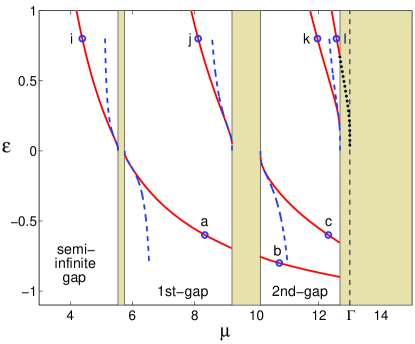
Figure 2: Bifurcations of defect modes with the defect described by Eq. (2.2) at $E_{0}=15$ and $I_{0}=6$. Solid lines: numerical results; dashed lines: analytical results. The shaded regions are the Bloch bands. Profiles of DMs at the circled points in this figure are displayed in Figs. 3 and 4.

As $|\epsilon|$ increases, DM branches move away from band edges (toward the left when $\epsilon>0$ and toward the right when $\epsilon<0$). Notice that in attractive defects ($\epsilon>0$), these branches stay inside their respective bandgaps. But in repulsive defects ($\epsilon<0$), DM branches march to edges of higher Bloch bands and then re-appear in higher bandgaps. For instance, the DM branch in the first bandgap reaches the edge of the second Bloch band at $\epsilon\approx-0.70$ and re-appears in the second bandgap when $\epsilon\approx-0.76$. These behaviors resemble those in the 1D case (see Fig. 4 in YangChendefect ). One difference between the 1D and 2D cases seems to be, in 1D repulsive defects, when DM branches approach edges of higher Bloch bands, the curves become tangential to the vertical band-edge line. This indicates that these 1D defect modes can not enter Bloch bands as embedded eigenvalues inside the continuous spectrum. This fact is consistent with the statement “(discrete) eigenvalues cannot lie in the continuous spectrum” in Beketov for locally perturbed periodic potentials in 1D linear Schrödinger equations. In the present 2D repulsive defects, on the other hand, the curves seem to intersect the vertical band-edge lines non-tangentially. This may lead one to suspect that these DM branches might enter Bloch bands and become embedded discrete eigenvalues. This suspicion appears to be wrong however for two reasons. First, the mathematical work by Kuchment and Vainberg Kuchment shows that for separable periodic potentials perturbed by localized defects, embedded DMs can not exist. In our theoretical model (2.5), the periodic potential is non-separable, thus their result does not directly apply. But their result strongly suggests that embedded DMs can not exist either in our case. Second, our preliminary numerical computations support this non-existence of embedded DMs. We find numerically that when a DM branch enters Bloch bands in Figure 2, the DM mode starts to develop oscillatory tails in the far field and becomes non-localized (thus not being a DM anymore).

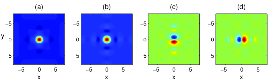
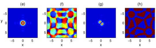
Figure 3: Profiles of defect modes in repulsive defects in Figure 2. (a)-(c): DMs at the circled points ‘a, b, c’ in Figure 2, with $(\epsilon,\mu)$=$(-0.6,8.33)$, $(-0.8,10.73)$, and $(-0.6,12.31)$, respectively; (d) the coexisting DM of mode (c); (e) and (f): intensity and phase of the vortex mode obtained by superimposing modes (c) and (d) with $\pi/2$ phase delay, i.e. in the form of $u(x,y)+iu(y,x)$; (g) and (h): intensity and phase of the diagonally-oriented dipole mode obtained by superimposing modes (c) and (d) with no phase delay, i.e. in the form of $u(x,y)+u(y,x)$.

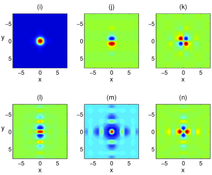
Figure 4: Profiles of defect modes in attractive defects in Figure 2. (i)-(l): DMs at the circled points ‘i, j, k, l’ in Figure 2, with $(\epsilon,\mu)$=(0.8, 4.39), (0.8, 8.12), (0.8, 11.96), and (0.8, 12.57), respectively. (m) and (n): DMs obtained by superimposing mode (l) and its coexisting mode with zero and $\pi$ phase delays, i.e. in the form of $u(x,y)+u(y,x)$ and $u(x,y)-u(y,x)$ respectively.

Now we examine profiles of defect modes on DM branches in Figure 2. For this purpose, we select one representative point from each DM branch, mark them by circles, and label them by letters in Figure 2. DM profiles at these marked points are displayed in Figs. 3 and 4. The letter labels for these defect modes are identical to those for the marked points on DM branches in Figure 2. First, we look at Figure 3, which shows DM profiles in repulsive defects $(\epsilon<0)$. We see that DMs at points ‘a, b’ of Figure 2 are symmetric in both $x$ and $y$, with a dominant hump at the defect site, and satisfy the relation $u(x,y)=u(y,x)$. These DMs are the simplest in their respective bandgaps, thus we will call them fundamental DMs. Notice that these fundamental DMs are sign-indefinite, i.e. they have nodes where the intensities are zero, because they do not lie in the semi-infinite bandgap. Although DMs in Figure 3(a, b) look similar, differences between them (mainly in their tail oscillations) do exist due to their residing in different bandgaps. These differences are qualitatively similar to the 1D case, which has been carefully examined before (see Fig. 8 (b, d) in YangChendefect and Fig. 4 (b, d) in Chen_OE ). The DM branch of point ‘c’ is more interesting. At each point on this branch, there are two linearly independent DMs, the reason being that this DM branch bifurcates from the right edge of the second Bloch band where two linearly independent Bloch modes exist (this band edge is a $X$ symmetry point, see Fig. 1). These two DMs are shown in Figure 3(c, d). One of them is symmetric in $x$ and anti-symmetric in $y$, while the other is opposite. They are related as $u(x,y)$ and $u(y,x)$ with $u(x,y)\neq u(y,x)$. These DMs are dipole-like. However, these dipoles are largely confined inside the defect site. They are closely related to certain single-Bloch-mode solitons reported in Shi .

Since the DM branch of point ‘c’ admits two linearly independent defect modes, their arbitrary linear superposition would remain a defect mode since Eq. (2.5) is linear. Such linear superpositions could lead to new interesting DM structures. For instance, if the two DMs in Figure 3(c, d) are superimposed with $\pi/2$ phase delay, i.e. in the form of $u(x,y)+iu(y,x)$, we get a vortex-type DM whose intensity and phase structures are shown in Figure 3(e, f). This vortex DM is strongly confined in the defect site and looks like a familiar vortex-ring. It is qualitatively similar to vortex-cell solitons in periodic lattices under defocusing nonlinearity as reported in Shi , as well as linear vortex arrays in defected lattices as observed in ChenYangPRL . However, it is quite different from the gap vortex solitons as observed in Segev_highervortex , where the vortex beam itself creates an attractive defect with focusing nonlinearity, while the vortex DM here is supported by a repulsive defect. If the two DMs in Figure 3(c, d) are directly superimposed without phase delays, i.e. in the form of $u(x,y)+u(y,x)$, we get a dipole-type DM whose intensity and phase profiles are shown in Figure 3(g, h). This dipole DM is largely confined in the defect site and resembles the DM of Figure 3(c, d), except that its orientation is along the diagonal direction instead. This dipole DM is qualitatively similar to dipole-cell solitons in uniform lattices under defocusing nonlinearity as reported in Shi . If the two DMs in Figure 3(c, d) are superimposed with $\pi$ phase delay, i.e. in the form of $u(x,y)-u(y,x)$, the resulting DM would also be dipole-like but aligned along the other diagonal axis. Such a DM is structurally the same as the one shown in Figure 3(g, h) in view of the symmetries of our defected lattice.

Now we examine DMs in attractive defects, which are shown in Figure 4. At point ‘i’ in the semi-infinite bandgap, the DM is bell-shaped and is strongly confined inside the defect site [see Figure 4(i)]. This mode is guided by the total internal reflection mechanism, which is different from the repeated Bragg reflection mechanism for DMs in higher bandgaps. On the DM branch of point ‘j’, there are two linearly independent DMs which are related as $u(x,y)$ and $u(y,x)$. One of them is shown in Figure 4(j). This mode is dipole-like and resembles the one in Figure 3(c). Linear superpositions of this mode $u(x,y)$ with its coexisting mode $u(y,x)$ would generate vortex- and dipole-like DMs similar to those in Figure 3(e, f, g, h). In particular, the vortex DM at this point ‘j’ would be qualitatively similar to the gap vortex soliton as observed in Segev_highervortex . On the DM branch of point ‘k’, a single DM exists. This is because the left edge of the third Bloch band where this branch of DM bifurcates from is located at the $M$ symmetry point of the Brillouin zone (see Fig. 1) and admits only a single Bloch mode. The DM at point ‘k’ is displayed in Figure 4(k). This mode is largely confined at the defect site and is quadrupole-like. On the DM branch of point ‘l’, two linearly independent DMs exist which are related as $u(x,y)$ and $u(y,x)$. One of them is shown in Figure 4(l). This mode is symmetric in both $x$ and $y$ directions and is tripolar-like (with three dominant humps). Unlike DMs at points ‘c, j’, this DM, superimposed with its coexisting mode with $\pi/2$ phase delay would not generate vortex modes, since this DM has non-zero intensity at the center of the defect. However, their superpositions with zero and $\pi$ phase delays, i.e. in the forms of $u(x,y)+u(y,x)$ and $u(x,y)-u(y,x)$ would lead to two structurally different defect modes, which are shown in Figure 4(m, n). The DM in Figure 4(m) has a dominant hump in the center of the defect, surrounded by a negative ring, and with weaker satellite humps further out. The DM in Figure 4(n) is quadrupole-like, but oriented differently from the quadrupole-like DM in Figure 4(k). These DMs resemble the spike-array solitons and quadrupole-array solitons in uniform lattices under focusing nonlinearity as reported in Shi .

Most of the DM branches in Figure 2 bifurcate from edges of Bloch bands. Even the branch of point ‘b’ in the second bandgap of Figure 2 can be traced to the DM bifurcation from the right edge of the first Bloch band. But there are exceptions. One example is the DM branch of point ‘l’ in the upper right corner of the second bandgap in Figure 2 (we will call it the ‘l’ branch below). This ‘l’ branch does not bifurcate from any Bloch-band edge. Careful examinations show that DMs on this branch closely resemble Bloch modes at the lowest $\Gamma$-symmetry point in the third Bloch band (see Figure 1). Thus this ‘l’ branch should be considered as bifurcating from that lowest $\Gamma$-symmetry point when $\epsilon\ll 1$. However, we see from Figure 1 that this lowest $\Gamma$-symmetry point is not an edge point of the third Bloch band. Even though it is a local edge (minimum) point of diffraction surfaces in the Brillouin zone, it still lies inside the third Bloch band. Let us call this type of points “quasi-edge points” of Bloch bands. Then the ‘l’ branch of DMs bifurcates from a quasi-edge point, not a true edge point, of a Bloch band! To illustrate this fact, we connected the ‘l’ branch to this quasi-edge $\Gamma$-symmetry point (at $\epsilon=0$) by dotted lines through a fitted function of the form (3.19) in Figure 2. This dotted line lies inside the third Bloch band. One question we can ask here is: what is the nature of this dotted line? Since it is inside the Bloch band, the mathematical results by Kuchment and Vainberg Kuchment suggest that it can not be a branch of embedded DMs. On the other hand, the ‘l’ DM branch in the second bandgap does bifurcate out along this route. Then how does the ‘l’ branch bifurcate from the quasi-edge point along this route? This question awaits further investigation. We note by passing that the $\Gamma$ and $M$ points inside the second Bloch band are also quasi-edge points (see Figure 1(a)). Additional DM branches may bifurcate from such quasi-edge points as well.

IV Dependence of defect modes on the applied dc field $E_{0}$

In the previous section, we investigated the bifurcation of DMs as the local-defect strength parameter $\epsilon$ varies. In experiments on photorefractive crystals, the applied dc field $E_{0}$ can be adjusted in a wide range much more easily than the defect strength. So in this section, we investigate how DMs are affected by the value of $E_{0}$ in Eqs. (2.1)-(2.2) under localized defects of (2.3). When $E_{0}$ changes, so does the lattice potential. We consider both attractive and repulsive defects at fixed values of $\epsilon=\pm 0.9$ (the reason for these choices of $\epsilon$ values will be given below). For other fixed $\epsilon$ values, the dependence of DMs on $E_{0}$ is expected to be qualitatively the same. The reader is reminded that throughout this section, the $I_{0}$ value is fixed at $I_{0}=6$.

IV.1 The case of repulsive defects

In 2D photonic lattices with single-site repulsive defects we experimentally created in ChenYangPRL , $\epsilon\approx-1$. At this value of $\epsilon$, however, we found that DMs may exist in high bandgaps, but not in low bandgaps (see Figure 2 where $E_{0}=15$). Thus for presentational purposes, we take $\epsilon=-0.9$ in our computations below. The corresponding lattice profile of $I_{L}(x,y)$ is shown in Figure 5(a), which still closely resembles the defects in our previous experiments ChenYangPRL .

For this defect, we found different types of defect modes at various values of $E_{0}$. The results are summarized in Figs. 5(b) and 6. In Figure 5(b), the dependence of DM eigenvalues $\mu$ on the dc field $E_{0}$ is displayed. As can be seen, when $E_{0}$ increases from zero, a DM branch appears in the second bandgap at $E_{0}\approx 8.5$. When $E_{0}$ increases further, this branch moves toward the third Bloch band and disappears at $E_{0}\approx 15$. But when $E_{0}$ increases to $E_{0}\approx 23.4$, another DM branch appears in the third bandgap. This branch moves toward the fourth Bloch band and disappears at $E_{0}\approx 36.7$. In the fourth gap, there are two DM branches. The upper branch exists when $45.9<E_{0}<64.2$, and the lower branch exists when $31.6<E_{0}<40.8$. As $E_{0}$ increases even further, DM branches will continue to migrate from lower bandgaps to higher ones. These behaviors are qualitatively similar to the 1D case (see Fig. 7 in YangChendefect ). Some examples of DMs marked by circles in Figure 5 are displayed in Figure 6. We can see that DMs at points ‘a, b, c’ are “fundamental” DMs. At point ‘d’, there are two linearly independent DMs related by $u(x,y)$ and $u(y,x)$, one of which is displayed in Figure 6(d). These DMs are dipole-like, similar to the ‘c’ branch in Figure 2. Linear superpositions of these DMs with $\pi/2$ and $0$ phase delays would generate a vortex DM and a diagonally-oriented dipole DM, whose amplitude profiles are shown in Figure 6 (e) and (f) (their phase fields are similar to those in Figure 3(f, h) and thus not shown here).

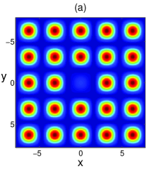
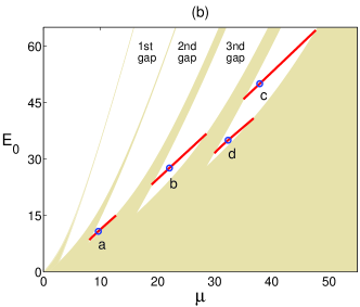
Figure 5: (a) Profile of the lattice $I_{L}(x,y)$ in Eq. (2.2) with a repulsive localized defect of (2.3) and $\epsilon=-0.9$ ($I_{0}=6$). (b) The corresponding DM branches in the $(\mu,E_{0})$ parameter space. Shaded: Bloch bands. DMs at the circled points are displayed in Figure 6.

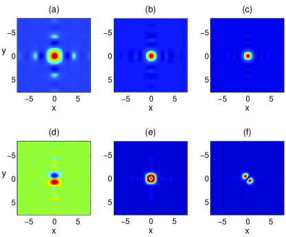
Figure 6: (a)-(d): Defect modes supported by the repulsive localized defect of Figure 5(a) at the circled points ‘a, b, c, d’ of Figure 5(b), with $(E_{0},\mu)$=(10.8, 9.61), (27.6, 22.06), (50.0, 37.88), and (35.0, 32.34), respectively. (e) and (f): Intensity profiles of the vortex and dipole modes obtained by superposing mode (d) and its coexisting mode with $\pi/2$ and zero phase delays.

IV.2 The case of attractive defects

For attractive defects, we choose $\epsilon=0.9$ following the above choice of $\epsilon=-0.9$ for repulsive defects. The lattice profile at this $\epsilon$ value is shown in Figure 7(a). The dependence of DM eigenvalues $\mu$ on the dc field $E_{0}$ is shown in Figure 7(b). Unlike DMs in repulsive defects, DMs in this attractive defect exist in all bandgaps (including the semi-infinite and first bandgaps). In addition, DM branches here stay in their respective bandgaps as $E_{0}$ increases, contrasting the repulsive case. DM profiles at marked points in Figure 7(b) are displayed in Figure 8. The DM in Figure 8(a) is bell-shaped and all positive, and it is the fundamental DM in the semi-infinite bandgap. This DM is similar to the one on the ‘i’ branch of Figure 2, and is guided by the total internal reflection mechanism. The DM in the first bandgap is dipole-like and is displayed in Figure 8(b). This DM branch is similar to the ‘j’ branch of Figure 2. On this branch, there is another coexisting DM which is a $90^{\circ}$-rotation of Figure 8(b). Linear superpositions of these two DMs could generate vortex-like and diagonally-oriented dipole-like DMs, as Figure 3(e, f, g, h) shows. In the second bandgap, there are two DM branches: the ‘c’ branch and the ‘d’ branch. DMs on the ‘c’ branch are quadrupole-like, and this branch is similar to the ‘k’ branch of Figure 2. On this branch, there is a single linearly independent defect mode. The ‘d’ branch is similar to the ‘l’ branch of Figure 2. On this branch, there are two linearly independent DMs which are tripolar-like and orthogonal to each other [see Figure 4(l)]. A superposition of these DMs with zero phase delay creates a hump-ring-type structure which is shown in Figure 8(d) [see also Figure 4(m)]. A different superposition would produce a quadrupole-type structure as the one shown in Figure 4(n). In the third and fourth bandgaps, there are additional DM branches. These branches exist at $E_{0}$ values higher than 15, thus have no counterparts in Figure 2 (where $E_{0}=15$). Profiles of these DMs are more exotic as can be seen in Figure 8 (e) and (f).

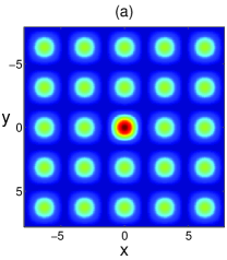
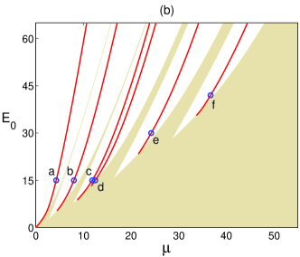
Figure 7: (a) Profile of the lattice $I_{L}(x,y)$ in Eq. (2.2) with an attractive localized defect of (2.3) and $\epsilon=0.9$ ($I_{0}=6$). (b) The corresponding DM branches in the $(\mu,E_{0})$ parameter space. Shaded: Bloch bands. DMs at the circled points are displayed in Figure 8.

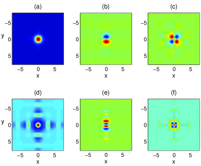
Figure 8: Defect modes supported by attractive localized defects of Figure 7(a) at the circled points ‘a, b, c, d, e, f’ of Figure 7(b), with $(E_{0},\mu)$=(15, 4.29), (15, 8.00), (15, 11.84), (15, 12.48), (30, 24.23) and (42, 36.69), respectively.

V Defect modes in non-localized defects

In previous sections, we exclusively dealt with defect modes in 2D-localized defects. We found that DM eigenvalues bifurcate out from Bloch-band edges exponentially with the defect strength $\epsilon$ [see Eq. (3.19)]. In addition, DMs can not be embedded inside Bloch bands (i.e. the continuous spectrum). In this section, we briefly discuss DMs in non-localized defects, and point out two significant differences between DMs in localized and non-localized defects. One is that in non-localized defects, DM eigenvalues can bifurcate out from edges of the continuous spectrum algebraically, not exponentially, with the defect strength $\epsilon$. The other one is that in non-localized defects, DMs can be embedded inside the continuous spectrum as embedded eigenmodes.

For simplicity, we consider the following linear Schrödinger equation with separable non-localized defects,

$$u_{xx}+u_{yy}+\left\{V_{D}(x)+V_{D}(y)\right\}u=-\mu u,$$ (5.1)

where function $V_{D}$ is a one-dimensional defected periodic potential of the form

$$V_{D}(x)=-\frac{E_{0}}{1+I_{0}\cos^{2}(x)\left\{1+\epsilon F_{D}(x)\right\}},$$ (5.2)

$F_{D}(x)=\mbox{exp}(-x^{8}/128)$ is a defect function as has been used before YangChendefect , and $\epsilon$ is the defect strength. We chose this separable defect in Eq. (5.1) because all its eigenmodes (both discrete and continuous) can be obtained analytically (see below). The non-localized nature of this separable defect can be visually seen in Figure 9(a), where the defected potential $V_{D}(x)+V_{D}(y)$ for $I_{0}=3,E_{0}=6$, and $\epsilon=-0.7$ is displayed. Note that this potential plotted here differs from the usual concept of quantum-mechanics potentials by a sign, and it resembles the refractive-index function in optics. We see that along the $x$ and $y$ axes in Figure 9(a), the defect extends to infinity (thus non-localized). The above $I_{0}$ and $E_{0}$ parameters were chosen because they have been used before in the 1D defect-mode analysis of YangChendefect , and such 1D results will be used to construct the eigenmodes of the 2D defect equation (5.1) below.

Since the potential in Eq. (5.1) is separable, the eigenmodes of this equation can be split into the following form:

$$u(x,y)=u_{a}(x)u_{b}(y),\quad\mu=\mu_{a}+\mu_{b},$$ (5.3)

where $u_{a},u_{b},\mu_{a},\mu_{b}$ satisfy the following one-dimensional eigenvalue equation:

$$u_{a,xx}+V_{D}(x)u_{a}=-\mu_{a}u_{a},$$ (5.4)

$$u_{b,yy}+V_{D}(y)u_{b}=-\mu_{b}u_{b}.$$ (5.5)

These two 1D equations for $u_{a}$ and $u_{b}$ are identical to the 1D defect equation we studied comprehensively in YangChendefect . Using the splitting (5.3) and the 1D results in YangChendefect , we can construct the entire discrete and continuous spectra of Eq. (5.1).

Before we construct the spectra of Eq. (5.1), we need to clarify the definitions of discrete and continuous eigenvalues of this 2D equation. Here an eigenvalue is called discrete if its eigenfunction is square-integrable (thus localized along all directions in the $(x,y)$ plane). Otherwise it is called continuous. Note that an eigenfunction which is localized along one direction (say $x$ axis) but non-localized along another direction (say $y$ axis) corresponds to a continuous, not discrete, eigenvalue.

Now we construct the spectra of Eq. (5.1) for a specific example with $E_{0}=6,I_{0}=3$ and $\epsilon=0.8$. At these parameter values, the discrete eigenvalues and continuous-spectrum intervals (1D Bloch bands) of the 1D eigenvalue problem (5.4) are (see YangChendefect )

$$\{\lambda_{1},\lambda_{2},\lambda_{3},\dots\}=\{2.0847,\;4.5002,\;7.5951,\dots,\},$$ (5.6)

$$\{[I_{1},I_{2}],\,[I_{3},I_{4}],\,[I_{5},I_{6}],\dots\}=\{[2.5781,\;2.9493],\;[4.7553,\;6.6010],\;[7.6250,\;11.8775],\dots\}.$$ (5.7)

Using the relation (5.3), we find that the discrete eigenvalues and continuous-spectrum intervals of the 2D eigenvalue problem (5.1) are

$$\{\mu_{1},\mu_{2},\mu_{3},\mu_{4},\dots\}=\{2\lambda_{1},\;\lambda_{1}+\lambda_{2},\;2\lambda_{2},\;\lambda_{1}+\lambda_{3},\dots\}=\{4.1694,\;6.5849,\;9.0004,\;9.6798,\dots,\},$$ (5.8)

and

$$\{\mu_{\mbox{continuum}}\}=\{[\lambda_{1}+I_{1},\>2I_{2}],\;[\lambda_{1}+I_{3},\>\infty)\}=\{[4.6628,\;5.8986],\;[6.8400,\;\infty)\}.$$ (5.9)

Note that at the left edges of the two continuous-spectrum bands ($\mu=4.6628$ and 6.8400), the eigenfunctions are non-localized along one direction but localized along its orthogonal direction, thus they are not the usual 2D Bloch modes (which would have been non-localized along all directions). This is why for Eq. (5.1), we do not call these continuous-spectrum bands as Bloch bands.

Repeating the same calculations to other $\epsilon$ values, we have constructed the whole spectra of Eq. (5.1) in the $(\mu,\epsilon)$ plane for $I_{0}=3$ and $E_{0}=6$. The results are displayed in Figure 9(b). Here solid curves show branches of DMs (discrete eigenvalues), and shaded regions are the continuous spectrum. This figure shows two significant features which are distinctively different from those in localized defects. One is that several DM branches (such as the ‘c’ and ‘d’ branches) are either partially or completely embedded inside the continuous spectrum. This means that in non-localized defects, embedded DMs inside the continuous spectrum do exist. This contrasts the localized-defect case, where the mathematical results of Kuchment and Vainberg Kuchment and our numerics show non-existence of embedded DMs. Another feature of Figure 9(b) is on the quantitative behavior of DM bifurcations from edges of the continuous spectrum at small values of the defect strength $\epsilon$. We have shown before that in the 1D case, DMs bifurcate out from Bloch-band edges quadratically with $\epsilon$ YangChendefect . For the 2D problem (5.1), using the relation (5.3), we can readily see that when DMs bifurcate out from edges of the continuous spectrum (see the ‘a, b, d’ branches for instance), the distance between DM eigenvalues and the continuum edges also depends on $\epsilon$ quadratically. This contrasts the localized-defect case, where we have shown in section III that DMs bifurcate out from Bloch-band edges exponentially.

Even though the defect in Eq. (5.1) is non-localized rather than localized, the DMs it admits actually are quite similar to those in localized defects. To demonstrate, we picked four representative points on the DM branches of Figure 9(b). These points are marked by circles and labeled by letters ‘a, b, c, d’ respectively. Profiles of DMs at these four points are displayed in Figure 10. Comparing these DMs with those of localized defects in Figs. 3 and 4, we easily see that they are quite similar. In particular, the ‘a, b, c, d’ branches in Figure 9(b) resemble the ‘i, j, k, a’ branches in Figure 2, as DMs on the corresponding branches are much alike. Notice that DMs in the non-localized defect case are a little more spread out than their counterparts in the local-defect case (compare Figs. 4(k) and 10(c), for instance). This is simply because in the non-localized defect, we chose $E_{0}=6$, while in the localized defect, we chose a much higher value of $E_{0}=15$. Higher $E_{0}$ values induce deeper potential variations, which facilitates better confinement of DMs. We need to point out that, even though the DMs at points ‘c, d’ are embedded inside the continuous spectrum, their eigenfunctions are perfectly 2D-localized and square-integrable (see Figure 10(d) in particular). Thus, the embedded nature of a defect mode does not necessarily cause it to spread out more.

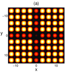
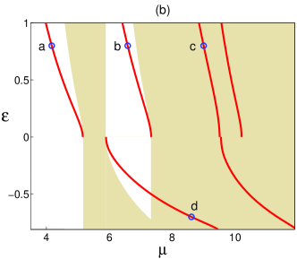
Figure 9: (a) Profile of a 2D potential with non-localized defects $V_{D}(x)+V_{D}(y)$ in Eqs. (5.1)-(5.2) with $E_{0}=6$, $I_{0}=3$, and $\epsilon=-0.7$. (b) DM branches supported by this non-localized defect in the $(\mu,\epsilon)$ parameter space. Shaded: the continuous spectrum. DMs at the circled points are displayed in Figure 10.

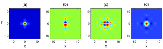
Figure 10: Defect modes in non-localized defects (5.1)-(5.2) at the circled points ‘a, b, c, d’ in Figure 9(b), with $(\epsilon,\mu)$=(0.8, 4.17), (0.8,6.59), (0.8, 9.00), and $(-0.7,8.61)$ respectively.

VI Summary

In summary, we have thoroughly investigated defect modes in two-dimensional photonic lattices with localized or non-localized defects. When the defect is localized and weak, we analytically determined defect-mode eigenvalues bifurcated from edges of Bloch bands. We found that in an attractive (repulsive) defect, defect modes bifurcate out from Bloch-band edges with normal (anomalous) diffraction coefficients. Furthermore, distances between defect-mode eigenvalues and Bloch-band edges are exponentially small functions of the defect strength, which is qualitatively different from the 1D case. Another interesting phenomenon we found was that, some defect-mode branches bifurcate not from Bloch-band edges, but from quasi-edge points within Bloch bands. When the defect is localized but strong, defect modes were studied numerically. It was found that both the repulsive and attractive defects can guide various types of defect modes such as fundamental, dipole, tripolar, quadrupole, and vortex modes. These modes reside in various bandgaps of the photonic lattice. As the defect strength increases, defect modes move from lower bandgaps to higher ones when the defect is repulsive, but remain within each bandgap when the defect is attractive. The same phenomena are observed when the defect is held fixed while the applied dc field increases. If the defect is non-localized (i.e. the defect does not disappear at infinity in the lattice), we showed that DMs exhibit two new features: (i) DMs can be embedded inside the continuous spectrum; (ii) DMs can bifurcate out from edges of the continuous spectrum algebraically rather than exponentially. These theoretical results pave the way for further experimental demonstrations of various type of DMs in a 2D lattice.

References

- (1) P.St.J. Russell, Science 299, 358 (2003).
- (2) J.D. Joannopoulos, R.D. Meade, J.N. Winn, Photonic Crystals: Molding the Flow of Light (Princeton University Press, Princeton, NJ, 1995).
- (3) D. N. Christodoulides, F. Lederer, and Y. Silberberg, Nature (London) 424, 817 (2003)
- (4) Y. S. Kivshar and G. P. Agrawal, Optical Solitons: From Fibers to Photonic Crystals (Academic Press, New York, 2003).
- (5) J.W. Fleischer, M. Segev, N.K. Efremidis, and D.N. Christodoulides, Nature 422, 147 (2003).
- (6) H. Martin, E.D. Eugenieva, Z. Chen and D.N. Christodoulides, “Discrete solitons and soliton-induced dislocations in partially-coherent photonic lattices, Phys. Rev. Lett. 92, 123902 (2004).
- (7) I. Makasyuk, Z. Chen and J. Yang, “Bandgap guidance in optically-induced photonic lattices with a negative defect”, Phys. Rev. Lett. 96, 223903 (2006).
- (8) X. Wang, J. Young, Z. Chen, D.Weinstein, and J. Yang, “Observation of lower to higher bandgap transition of one-dimensional defect modes”, Opt. Exp. 14, 7362-7367 (2006).
- (9) F. Fedele, J. Yang, and Z. Chen, “Defect modes in one-dimensional photonic latices.” Opt. Lett. 30, 1506 (2005).
- (10) F. Fedele, J. Yang, and Z. Chen, “Properties of defect modes in one-dimensional optically-induced photonic latices.” Stud. Appl. Math. 115, 279-301 (2005)
- (11) A. A. Sukhorukov and Y. S. Kivshar, “Nonlinear localized waves in a periodic medium”, Phys. Rev. Lett. 87, 083901 (2001).
- (12) J. Yang and Z. Chen, “Defect solitons in photonic lattices.” Phys. Rev. E 73, 026609 (2006).
- (13) U. Peschel, R. Morandotti, J. S. Aitchison, H. S. Eisenberg, and Y. Silberberg, Appl. Phys. Lett. 75, 1348 (1999).
- (14) H.S. Eisenberg, Y. Silberberg, R. Morandotti, A. R. Boyd, and J. S. Aitchison, “Observation of discrete solitons in optical waveguide arrays, Phys. Rev. Lett. 81, 3383 (1998).
- (15) D.N. Neshev, E. Ostrovskaya, Y. Kivshar, and W. Krolikowski, “Spatial solitons in optically induced gratings”, Opt. Lett. 28, 710 (2003).
- (16) J. Yang, I. Makasyuk, A. Bezryadina, and Z. Chen, “Dipole and quadrupole solitons in optically-induced two-dimensional photonic lattices: theory and experiment.” Stud. Appl. Math. 113, 389 (2004).
- (17) J. Yang and Z. Musslimani, “Fundamental and vortex solitons in a two-dimensional optical lattice.” Opt. Lett. 28, 2094 (2003).
- (18) D.N. Neshev, T.J. Alexander, E.A. Ostrovskaya, Y.S. Kivshar, H. Martin, I. Makasyuk, Z. Chen, Observation of discrete vortex solitons in optically-induced photonic lattices, Phys. Rev. Lett. 92, 123903 (2004).
- (19) J.W. Fleischer, G. Bartal, O. Cohen, O. Manela, M. Segev, J. Hudock, D.N. Christodoulides, Observation of vortex-ring discrete solitons in 2D photonic lattices. Phys. Rev. Lett. 92, 123904 (2004).
- (20) G. Bartal, O. Manela, O. Cohen, J.W. Fleischer, and M. Segev, “Observation of Second-Band Vortex Solitons in 2D Photonic Lattices”, Phys. Rev. Lett. 95, 053904 (2005).
- (21) R. Fischer, D. Trager, D.N. Neshev, A.A. Sukhorukov, W. Krolikowski, C. Denz, and Y.S. Kivshar, “Reduced-Symmetry Two-Dimensional Solitons in Photonic Lattices”, Phys. Rev. Lett. 96, 023905 (2006).
- (22) Z. Shi, J. Yang and Z. Chen, “Solitary Waves Bifurcated from Bloch Bands in Two-dimensional Periodic Media”, preprint.
- (23) Y.V. Kartashov, V.A. Vysloukh, and L. Torner, “Rotary Solitons in Bessel Optical Lattices”, Phys. Rev. Lett. 93, 093904 (2004).
- (24) X. Wang, Z. Chen, and P. G. Kevrekidis, “Observation of discrete solitons and soliton rotation in periodic ring lattices”, Phys. Rev. Lett. 96, 083904 (2006).
- (25) M.J. Ablowitz, B. Ilan, E. Schonbrun, and R. Piestun, “Solitons in two-dimensional lattices possessing defects, dislocations, and quasicrystal structures”, Phys. Rev. E 74, 035601 (2006).
- (26) D. E. Pelinovsky, A. A. Sukhorukov, and Y. S. Kivshar, “Bifurcations and stability of gap solitons in periodic potentials”, Phys. Rev. E 70, 036618 (2004).
- (27) D. N. Christodoulides and M. I. Carvalho, J. Opt. Soc. Am. B 12, 1628 (1995).
- (28) M. Segev, M. Shih, and G. C. Valley, J. Opt. Soc. Am. B 13, 706 (1996).
- (29) D.E. Pelinovsky and C. Sulem, “Asymptotic approximations for a new eigenvalue in linear problems without a threshold”, Theor. Math. Phys. 122, 98-106 (2000).
- (30) J. Yang and T.I. Lakoba, “Universally-convergent squared-operator iteration methods for solitary waves in general nonlinear wave equations”, Stud. Appl. Math. 118, 153-197 (2007).
- (31) F. Odeh and J.B. Keller, “Partial differential equations with periodic coefficients and Bloch waves in crystals.” J. Math. Phys. 5, 1499 (1964).
- (32) F. S. Rofe-Beketov, “A test for the finiteness of the number of discrete levels introduced into the gaps of a continuous spectrum by perturbations of a periodic potential”, Soviet Math. Dokl. 5, 689-692 (1964).
- (33) P. Kuchment and B. Vainberg, “On absence of embedded eigenvalues for Schr dinger operators with perturbed periodic potentials”, Commun. Part. Diff. Equat. 25, 1809 - 1826 (2000).