Experiments on the twisted vortex state in superfluid ³He-B

Abstract

We have performed measurements and numerical simulations on a bundle of vortex lines which is expanding along a rotating column of initially vortex-free ³He-B. Expanding vortices form a propagating front: Within the front the superfluid is involved in rotation and behind the front the twisted vortex state forms, which eventually relaxes to the equilibrium vortex state. We have measured the magnitude of the twist and its relaxation rate as function of temperature above $0.3\,T_{\rm c}$. We also demonstrate that the integrity of the propagating vortex front results from axial superfluid flow, induced by the twist.

PACS numbers: 67.57.Fg, 47.32.y, 67.40.Vs

1 Introduction

Since the pioneering works by Feynman, and by Hall and Vinen a rotating superfluid has been associated with an array of rectilinear vortex lines, stretched along the axis of rotation. This lowest energy state is known as the equilibrium vortex state. Different kinds of collective excitations of vortex arrays have been discussed over the years sonin , including analogs of Kelvin waves on bundles of vortices vw ; henderson and Tkachenko waves tkwpred ; tkwobserv . Recently a new state of vortex matter, the twisted vortex state, was experimentally identified and theoretically described in the B phase of superfluid ³He twistprl . In this state vortices have helical configuration circling around the axis of rotation. Remarkably, certain such configurations, uniform in the direction of the rotation axis, do not decay, although the energy of this state is higher than that of the equilibrium vortex array. The reason is that the force, acting on vortices, is directed along the vortex cores everywhere.

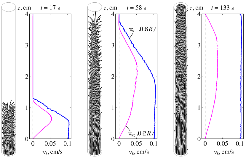
Figure 1: (Color online) Numerical simulations of vortex dynamics demonstrate the twisted vortex state during the expansion of the vortex bundle along the rotating column. The subsequent relaxation of the twisted state proceeds from the top and bottom sample boundaries. The vortex configuration and the $z$-dependencies of the superfluid velocity components at given radial distance are shown at three points in time. The sample radius is 1.5 mm, length 40 mm, angular velocity 1 rad/s and temperature $0.5\,T_{\rm c}$.

The twisted vortex state is created when a bundle of vortex lines expands along an initially vortex-free rotating superfluid column, Fig. 1. Those segments of the vortex lines, which terminate on the side wall of the sample cylinder, propagate towards the vortex-free part and simultaneously precess around the central axis under the action of the Magnus and mutual friction forces. Such two-component motion leads to a vortex bundle which is helically twisted. Expansion along the column becomes slower with decreasing temperature as mutual friction decreases. Thus the spiral, created by the motion of the vortex end on the side wall, becomes tighter. One may expect that the resulting twist, characterized by the wave vector $Q$ of the vortex helix in the bundle, becomes stronger as the temperature is reduced. We have measured the magnitude of the twist in the range 0.3 – 0.8 $T_{\rm c}$ and observed this expected behavior only at $T>0.45\,T_{\rm c}$. Below $0.45\,T_{\rm c}$ the magnitude of the twist decreases again.

In the real sample, which is not infinitely long, the twist cannot be completely uniform: At the top and bottom ends of the sample the vortices are perpendicular to the wall and the twist disappears there. The twist in the bulk unwinds when the vortex ends slide over the end plates of the sample cylinder. The model in Ref. twistprl predicts that the relaxation of the twist becomes faster with decreasing temperature and distance to the wall. We have experimentally confirmed both properties and established reasonable agreement with the model.

We also examine in this report the role of the twist-induced superflow in the propagation of the vortex front, which separates the vortex-free superfluid from the twisted vortex bundle. At $T\gtrsim 0.45\,T_{\rm c}$ the thickness of the vortex front increases while it propagates. At lower temperatures the twist-induced axial superflow pushes vortices at the rear of the front forward. Eventually they catch up with the vortices in the head of the front and the front propagates in a thin steady-state configuration.

2 Numerical simulations

The essential features of the vortex front and the twisted state can be displayed by means of numerical calculations of vortex dynamics in a rotating cylinder. The simulation technique accounts fully for inter-vortex interaction and for the effect of solid walls simul . In the initial state at $t=0$ the equilibrium number of vortices is placed as quarter-loops between the bottom and the cylindrical walls. During the subsequent evolution one observes the formation of the vortex front and a twisted cluster behind it, Fig. 1. The profile of the azimuthal component of the superfluid velocity $v_{{\rm s}\phi}$ shows an almost linear transition from the non-rotating state $v_{{\rm s}\phi}=0$ to equilibrium rotation $v_{{\rm s}\phi}\approx\Omega r$ within the region of the vortex front. This shear flow within the front is created by vortices which terminate on the cylindrical wall perpendicular to the axis of rotation. At the temperature of $0.5\,T_{\rm c}$ the thickness of the vortex front grows with time. Simulations at $0.4\,T_{\rm c}$ on the other hand demonstrate a thin time-invariant front twistprl . We discuss this difference below.

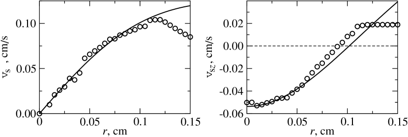
Figure 2: Radial dependencies of the superfluid velocity from the simulation snapshot in the center panel of Fig. 1. Circles are the simulation results at $z=1.8\,$cm, averaged over the azimuthal angle. Lines are fit to the twist model Eq. (1) with $Q=0.776R^{-1}$. At $r>0.12\,$cm the simulation results display the equilibrium vortex-free region around the central vortex cluster. This feature is ignored in the analytic model.

The appearance of the twist is reflected in the axial superflow at the velocity $v_{{\rm s}z}$, which is along the vortex expansion direction close to the cylindrical boundary and in the opposite direction close to the axis. As shown in Fig. 2, at constant height $z$ the $r$-dependencies of $v_{{\rm s}\phi}$ and $v_{{\rm s}z}$ are reasonably well described by the model suggested in Ref. twistprl :

$$v_{{\rm s}\phi}(r)=\frac{(\Omega+Qv_{0})r}{1+Q^{2}r^{2}},\ \ v_{{\rm s}z}(r)=\frac{v_{0}-Q\Omega r^{2}}{1+Q^{2}r^{2}},$$ (1)

where $v_{0}=(\Omega/Q)[Q^{2}R^{2}/\ln(1+Q^{2}R^{2})-1]$ and $R$ is the sample radius. The wave vector $Q$ of the twist has its maximum value close to the rear end of the front and decreases to zero at the bottom and top ends of the sample. The axial superflow affects the NMR spectrum of ³He-B and this allows us to observe the twisted vortex state in the experiment.

3 Experiment

The experimental techniques are similar to those in the recent studies of non-equilibrium vortex dynamics in ³He turbreview . The sample of ³He-B at 29 bar pressure is contained in a cylindrical smooth-walled container with dimensions shown in Fig. 3. The sample is split in two independent B-phase volumes by an A phase layer, stabilized with applied magnetic field. In each B-phase volume an independent NMR spectrometer is used to monitor the vortex configuration. Two arrangements for pick-up coils have been used. They are labelled throughout this report as “setup 1” and “setup 2”. These arrangements differ in the placement of the pick-up coils with respect to the upper and lower ends of the container, in Larmor frequencies, in the design of pick-up coils, and in the field homogeneity. The last property is mostly determined by the field distortion from the superconducting wire in the pick-up coils. For solenoidal coils in setup 1 it is $\Delta H/H\approx 6\cdot 10^{-4}$, while the coils in setup 2 distort the field more and $\Delta H/H\approx 1.7\cdot 10^{-3}$.

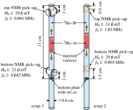
Figure 3: (Color online) Experimental setup.

The initial vortex-free state is prepared by thermal cycling of the sample to temperatures above $0.7\,T_{\rm c}$, where one waits at $\Omega=0$ for the annihilation of the dynamic remanent vortices left over from the previous experiment dyn-remn . After that the sample is cooled in rotation at $\Omega=0.8\,$rad/s to the target temperature.

For vortex injection the angular velocity is ramped with the rate $\dot{\Omega}=0.03\,$rad/s² above the critical velocity of the AB interface instability $\Omega_{\rm cAB}$ ABinstab , after which $\Omega$ is kept constant, Fig. 4. In the instability event about 10 vortices are injected into the B-phase close to the AB interface. At $T<0.6\,T_{\rm c}$ a turbulent burst immediately follows and generates almost the equilibrium number of vortices measturb . These vortices then propagate towards the pick-up coil. The instability velocity $\Omega_{\rm cAB}$ is controlled by temperature and magnetic field profile and varies between 1.1 and 1.5 rad/s. A modification of this injection technique has been used at $T>0.6\,T_{\rm c}$. Here the sample initially rotates at $\Omega>2\,$rad/s without the A phase. Then the magnetic field is increased until the formation of the A phase starts. The AB interface immediately goes unstable and hundreds of vortices are generated injLT .

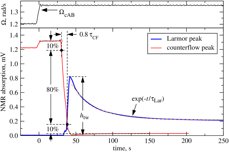
Figure 4: (Color online) Examples of NMR records from a vortex injection experiment and definition of the parameters $\tau_{\rm CF}$, $\tau_{\rm Lar}$ and $h_{\rm tw}$. The signal traces are recorded with the bottom spectrometer in setup 2 at $T=0.50\,T_{\rm c}$.

While vortices expand along the sample column and pass through the pick-up coil their configuration is read using NMR. The signal is measured at a fixed frequency either at the location of the counterflow or the Larmor peak in the NMR spectrum measturb . Absorption at the counterflow peak is sensitive to the difference in azimuthal flow velocities of the normal and superfluid components $v_{{\rm n}\phi}-v_{{\rm s}\phi}$. It is at maximum in the initial vortex-free state with $v_{{\rm s}\phi}=0$. When $v_{{\rm s}\phi}$ increases the absorption decreases rapidly and drops to zero when $v_{{\rm s}\phi}\sim(1/2)v_{{\rm n}\phi}$ juhacalc . Absorption in the Larmor peak is mostly sensitive to the axial flow $v_{{\rm s}z}$. It is zero in the vortex-free state while for a vortex cluster it has some finite value, which increases monotonously with increasing $v_{{\rm s}z}$ juhacalc .

An example of NMR measurement is presented in Fig. 4. To record signals at both Larmor and counterflow peaks with the same spectrometer the experiment is repeated twice in identical conditions. A rapid drop in the counterflow signal is seen which corresponds to the passage of the vortex front through the coil. We characterize this drop with time $\tau_{\rm CF}$. The Larmor peak grows first to a maximum value $h_{\rm tw}$, which corresponds to the maximum twist. Then the signal relaxes exponentially with the time constant $\tau_{\rm Lar}$ to a value characteristic for an equilibrium vortex cluster. The propagation velocity $V_{\rm f}$ of the vortices at the head of the front can be determined from their flight time between the injection moment, where $\Omega(t)=\Omega_{\rm cAB}$, and the arrival to the edge of the peak-up coil, as monitored with the counterflow peak. We do not discuss $V_{\rm f}$ in detail in this report.

4 Results

The temperature dependence of the magnitude of the twist is presented in Fig. 5. From the experiment the raw data are plotted: The maximum height of the Larmor peak $h_{\rm tw}$ (Fig. 4), normalized to the height of the Larmor peak at $\Omega=0$ at the same temperature. The data obtained in setup 1 and setup 2 are not identical since the spectrum shape around the Larmor peak depends on the magnitude of the magnetic field via the order parameter texture and also the homogeneity of the magnetic field is important: In setup 2 the homogeneity is worse and the Larmor peak cannot grow as high (i.e. as narrow) as in setup 1. Anyway, a clear maximum in the twist-induced signal is observed at around $0.45T_{\rm c}$. The same behavior of the magnitude of the twist is confirmed in the numerical simulations: The maximum value of the twist wave vector behind the front, as determined from a fit of the velocity profiles to Eq. (1), also peaks at $0.45T_{\rm c}$.

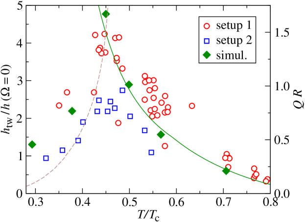
Figure 5: (Color online) Strength of the twist as a function of temperature. The measurements are performed using the bottom spectrometer in both setups of Fig. 3. The ratio of the maximum amplitude of the Larmor peak in the twisted state to the amplitude of the Larmor peak in the nonrotating sample is plotted on the left axis. The maximum value of the twist wave vector $Q$, obtained in simulations, is plotted on the right axis. The solid curve shows the fit $Q\,R=0.7(1-\alpha^{\prime})/\alpha$. The broken curve shows the minimum magnitude of the twist for which propagation of the vortex front in a thin steady-state configuration is possible.

The initial growth of the twist with decreasing temperature is expected. From the equations of motion of a single vortex which ends on the cylindrical wall, the estimate for the expansion velocity along $z$ is

$$v_{{\rm L}z}=\alpha(T)\,[v_{{\rm n}\phi}(R)-v_{{\rm s}\phi}(R)],$$ (2)

where $\alpha$ is a mutual friction coefficient bevan . As the normal fluid velocity at the side wall $v_{{\rm n}\phi}(R)=\Omega R$ and the superfluid velocity induced by a single vortex can be neglected in our conditions, Eq. (2) gives $v_{{\rm L}z}\approx\alpha\Omega R$. For the azimuthal velocity of the vortex end in the rotating frame a similar estimation gives $v_{{\rm L}\phi}\approx(1-\alpha^{\prime})\Omega R$, where $\alpha^{\prime}$ is another mutual friction coefficient bevan . Thus the trajectory of the vortex end on the side wall is a spiral with wave vector $Q=v_{{\rm L}\phi}/(Rv_{{\rm L}z})\approx(1-\alpha^{\prime})/(R\alpha)$. This value can be used as a rough estimation of the $Q$ vector in the twisted vortex state. As one sees from Fig. 5, the simulation results at $T\gtrsim 0.45\,T_{\rm c}$ indeed follow this dependence.

For the decreasing twist at $T<0.45\,T_{\rm c}$ a couple of reasons can be suggested. First, the twist can relax through reconnections between vortices in the bundle, which become more prominent with decreasing temperature. Second, relaxation of the twist proceeds in diffusive manner within the twisted cluster. The source of the twist is at the vortex front, while the sink is at the end plate of the cylinder, where the twist vanishes because of the boundary conditions. The effective diffusion coefficient increases as the temperature decreases twistprl . The faster diffusion limits the maximum twist in the finite-size sample at low temperatures.

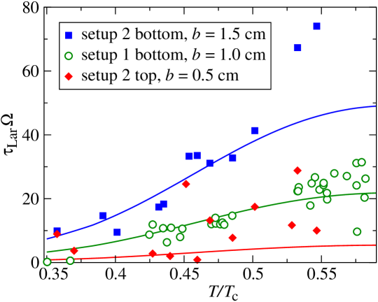
Figure 6: (Color online) Relaxation time of the twist versus temperature. Solid lines are fit to Eq. (3) with $C=2$.

The relaxation of the twisted state is observed as a decay in the amplitude of the Larmor peak. The measured time constant $\tau_{\rm Lar}$ of the exponential decay is presented in Fig. 6 for three different positions of the detector coil with respect to the end plate of the sample cylinder. It is clear that the relaxation indeed becomes faster with decreasing temperature. It is also evident that the relaxation of the twist proceeds faster as the observation point moves closer to the end plate of the sample cylinder. Both of these features are well described by the model presented in Ref. twistprl . According to this model the relaxation time of the twist is

$$\tau\approx\frac{C}{\Omega}\left(\frac{b}{R}\right)^{2}\frac{\alpha}{[(1-\alpha^{\prime})^{2}+\alpha^{2}]},$$ (3)

where $C\sim 1$ and $b$ is the distance along $z$ to the end plate, where the twist vanishes. The fit to this model using $C$ as the only fitting parameter demonstrates reasonable agreement with the measurements in Fig. 6. The experimental points show somewhat faster temperature dependence than the model. The discrepancy may result from shortcomings of both the model and the experiment. The model is constructed for the case of weak twist ($QR\ll 1$). In the experiment the probe is not point-like, but has a height comparable to the value of $b$ itself.

When Eq. (2) is applied to vortices within the vortex front, the following problem arises: At the head of the front the superfluid component is almost at rest, $v_{{\rm s}\phi}\ll v_{{\rm n}\phi}$, and the expansion velocity of vortices is $V_{\rm f}\approx\alpha\Omega R$. Behind the front the density of vortices is close to the equilibrium and $v_{{\rm s}\phi}\approx v_{{\rm n}\phi}$. Thus vortices at the tail of the front are barely able to expand and the thickness of the front should rapidly increase in time. On the other hand simulations show that vortices at the tail of the front do expand, Fig. 1. Moreover, at sufficiently low temperatures the expansion velocity of these vortices reaches the velocity of the foremost vortices, so that the front propagates in a thin steady-state configuration twistprl .

The explanation is that the vortex state behind the front is not the equilibrium state, but the twisted vortex state. Taking into account the axial superflow, induced by the twist, Eq. (2) should be modified as $v_{{\rm L}z}=\alpha\,[v_{{\rm n}\phi}(R)-v_{{\rm s}\phi}(R)]+(1-\alpha^{\prime})v_{{\rm s}z}(R)$. Given that $v_{{\rm s}z}(R)$ is in the direction of the front propagation and $v_{{\rm s}\phi}(R)<v_{{\rm n}\phi}(R)$ in the twisted state, the expansion velocity $V_{\rm t}$ of the vortices in the tail of the front is enhanced. This velocity can be estimated taking $v_{{\rm s}z}(R)$ and $v_{{\rm s}\phi}(R)$ from Eq. (1):

$$V_{\rm t}=\alpha\Omega R\left[1+\frac{1-\alpha^{\prime}}{\alpha}\,\frac{1}{Q\,R}\right]\,\left[1-\frac{Q^{2}R^{2}}{(1+Q^{2}R^{2})\,\log(1+Q^{2}R^{2})}\right]$$ (4)

This velocity has a maximum as a function of the $Q$ vector. If $\alpha/(1-\alpha^{\prime})>0.52$ (i.e. $T>0.46\,T_{\rm c}$ bevan ), the maximum value of $V_{\rm t}$ is less than the velocity of the foremost vortices $V_{\rm f}\approx\alpha\Omega R$. In these conditions the thickness of the front increases while it propagates. When $T<0.46\,T_{\rm c}$ a wide range of $Q$ values exists for which formally $V_{\rm t}\geqslant V_{\rm f}$. The minimum possible value of $Q$ is shown in Fig. 5 by the broken curve. In these conditions the vortex front propagates in a steady-state “thin” configuration. These simple considerations become inapplicable, however, when vortices interact strongly within the thin layer. To determine, say, the stable front thickness and the magnitude of the twist in the regime below $0.46\,T_{\rm c}$ a different approach would be needed.

The change in the front propagation at $T\approx 0.45\,T_{\rm c}$ is observed in both experiment and simulations. In the experiment the decay time of the counterflow peak $\tau_{\rm CF}$ in Fig. 4 can be used to extract the front thickness. The decay of the counterflow peak starts when the head of the vortex front arrives at that edge of the detector coil, which is closer to the injection point. The counterflow signal vanishes when the last part of the front, which still possesses enough counterflow to generate the NMR response, leaves the far edge of the detector coil. The product $\tau_{\rm CF}V_{\rm f}$ has the dimension of length and can be called the apparent thickness of the front. When the real thickness of the front grows with time its apparent thickness depends on the distance of the observation point from the injection point and on the rate with which the real thickness increases. When the front remains thin the value of its apparent thickness equals the height of the pick-up coil $d_{\rm coil}=9\,$mm.

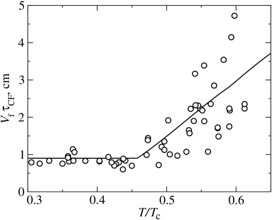
Figure 7: Apparent thickness of the vortex front as function of temperature. The solid line is the prediction of the model in Eq. (5).

The measurements of the apparent thickness of the front are presented in Fig. 7. The scatter at higher temperatures has two sources. Partially it is due to the uncertainty in the determination of $V_{\rm f}$ from flight times which are not long compared to the measuring resolution. Another contribution is the variation in the decay profile of the counterflow signal which may display weak oscillations around a roughly linear decrease. At $T>0.45T_{\rm c}$ we have $\tau_{\rm CF}V_{\rm f}>d_{\rm coil}$ and the apparent thickness decreases with temperature. Finally at $T<0.45\,T_{\rm c}$ the front becomes thin compared to the height of the pick-up coil. Assuming that at the moment of injection the front is infinitely thin we can write

$$\tau_{\rm CF}=\frac{d+d_{\rm coil}}{V_{\rm t}^{*}}-\frac{d}{V_{\rm f}},$$ (5)

where $d$ is the distance from the injection point (i.e. position of the AB interface) to the nearest edge of the pick-up coil and $V_{\rm t}^{*}$ is the expansion velocity at the position in the front where the NMR signal from the counterflow vanishes. Given that the latter condition roughly corresponds to $v_{{\rm s}\phi}\sim(1/2)v_{{\rm n}\phi}$ we take $V_{\rm t}^{*}=(V_{\rm t}+V_{\rm f})/2$ if $V_{\rm t}<V_{\rm f}$ and simply $V_{\rm t}^{*}=V_{\rm f}$ otherwise. Using $V_{\rm t}$ from Eq. (4) and the simple estimates $QR=(1-\alpha^{\prime})/\alpha$ and $V_{\rm f}=\alpha\Omega R$, we get from Eq. (5) the solid line in Fig. 7, which is in reasonable agreement with the experiment.

In the simulations the thickness of the front grows with time at higher temperatures. This process slows down as the twist increases with decreasing temperature (Fig. 5). Finally at $T\approx 0.45\,T_{\rm c}$ the twist reaches the value which is enough, according to Eq. (4), to support a thin front configuration. At lower temperatures the thickness of the front indeed becomes time-independent and roughly equal to the radius of the sample. Simultaneously the twist behind the front starts to drop, as has been discussed above. It remains, however, within the limits where the twist-induced superflow is able to keep the front thin.

5 Conclusions

We have studied the formation and relaxation of the twisted vortex state in ³He-B in the temperature range between $0.3\,T_{\rm c}$ and $0.8\,T_{\rm c}$. At higher temperatures $T\gtrsim 0.45\,T_{\rm c}$ the twist behind the propagating vortex front grows with decreasing temperature as $Q\propto(1-\alpha^{\prime})/\alpha$. Here the thickness of the front increases while it propagates along the rotating column. The axial superflow, induced by the twisted state, boosts the expansion velocity of vortices in the tail of the front. This enhancement increases as the twist grows with decreasing temperature. Finally at $T\approx 0.45\,T_{\rm c}$ vortices in the tail of the front are able to catch up with vortices in the head. At lower temperatures the front propagates in a thin steady-state configuration, while the twist starts to decrease.

The relaxation of the twist in a sample of finite length is not related to the front. It proceeds from the walls which limit the length of the sample along the rotation axis. The relaxation speeds up with decreasing temperature, unlike many other processes in vortex dynamics.

While the understanding of the front propagation and of the formation of the twisted vortex state in the high-temperature regime $T\gtrsim 0.45\,T_{\rm c}$ is quite good, in the low-temperature regime of a thin front the theoretical understanding is lacking. Especially interesting would be to consider the role of vortex reconnections and turbulence, both of which should increase with decreasing temperature.

References

- (1) E.B. Sonin, Rev. Mod. Phys. 59, 87 (1987).
- (2) H.E. Hall, Advan. Phys. 9, 89 (1960); E.L. Andronikashvili and J.S. Tsakadze, Zh. Eksp. Teor. Fiz. 37, 322 (1959) [Sov. Phys. JETP 10, 227 (1960)].
- (3) K.L. Henderson and C.F. Barenghi, Europhys. Lett. 67, 56 (2004).
- (4) V.K. Tkachenko, Zh. Eksp. Teor. Fiz. 50, 1573 (1966) [Sov. Phys. JETP 23, 1049 (1966)].
- (5) I. Coddington, P. Engels, V. Schweikhard, and E.A. Cornell, Phys. Rev. Lett. 91, 100402 (2003).
- (6) V.B. Eltsov, A.P. Finne, R. Hänninen, J. Kopu, M. Krusius, M. Tsubota, and E.V. Thuneberg, Phys. Rev. Lett. 96, 215302 (2006).
- (7) R. Hänninen, A. Mitani and M. Tsubota, J. Low Temp. Phys. 138, 589 (2005).
- (8) A.P. Finne, V.B. Eltsov, R. Hänninen, N.B. Kopnin, J. Kopu, M. Krusius, M. Tsubota and G.E. Volovik, Rep. Prog. Phys. 69, 3157 (2006).
- (9) R.E. Solntsev, R. de Graaf, V.B. Eltsov, R. Hänninen and M. Krusius, J. Low Temp. Phys. 149, in press Nos. 3/4 (2007).
- (10) R. Blaauwgeers, V.B. Eltsov, G. Eska, A.P. Finne, R.P. Haley, M. Krusius, J.J. Ruohio, L. Skrbek, and G.E. Volovik, Phys. Rev. Lett. 89, 155301 (2002).
- (11) A.P. Finne, S. Boldarev, V.B. Eltsov, and M. Krusius, J. Low Temp. Phys. 136, 249 (2004).
- (12) A.P. Finne, R. Blaauwgeers, S. Boldarev, V.B. Eltsov, J. Kopu, and M. Krusius, AIP Conf. Proc. 850, 177 (2006).
- (13) J. Kopu, J. Low Temp. Phys. 146, 47 (2007).
- (14) T.D.C. Bevan, A.J. Manninen, J.B. Cook, H. Alles, J.R. Hook and H.E. Hall, J. Low Temp. Phys. 109, 423 (1997).