Nonclassical dynamics of Bose condensates in an optical lattice in the superfluid regime

Abstract

A condensate in an optical lattice, prepared in the ground state of the superfluid regime, is stimulated first by suddenly increasing the optical lattice amplitude and then, after a waiting time, by abruptly decreasing this amplitude to its initial value. Thus the system is first taken to the Mott regime and then back to the initial superfluid regime. We show that, as a consequence of this nonadiabatic process, the system falls into a configuration far from equilibrium whose superfluid order parameter is described in terms of a particular superposition of Glauber coherent states that we derive. We also show that the classical equations of motion describing the time evolution of this system are inequivalent to the standard discrete nonlinear Schrödinger equations. By numerically integrating such equations with several initial conditions, we show that the system loses coherence, becoming insulating.

I Introduction

Nowadays Bose-Einstein condensates (BECs) represent one of more powerful and versatile testing grounds for low-energy modern physics in which experimental tests on quantum computation Mandel_Nature425 , many-body physics Mandel_PRL91 , superfluidity Burger_PRL86 , the Josephson junction effect Cataliotti_Science293 , atom optics Ottl_PRL95 , and quantum phase transitions Greiner_Nature415 can be performed. Condensates can be put into interaction with each other or manipulated by means of optical lattices (OLs), which are periodic trapping potentials generated by standing laser waves. By raising the amplitude of the OL, a condensate loaded therein is fragmented into an array of interacting condensates. By adjusting the laser amplitudes, the system is taken into different regimes. The superfluid regime is obtained with weak optical potentials (OPs), where the kinetic energy dominates over the interacting one, and the atoms hop from one well to another. The opposite -quantum- regime, is generated by strong OPs that suppress the tunneling of the atoms between the wells.

In this paper, we consider a one-dimensional gas. This is prepared by use of a transverse harmonic confining potential that tightly confines the atoms so that their motion, in the transverse direction, is limited to the zero point. Along the longitudinal direction, a further harmonic potential weakly confines the atoms, and an OP is switched on. For large enough laser amplitudes, the condensate splits into components tightly confined at the minima of the effective potential. In what follows, we imagine abruptly adjusting the amplitude of the longitudinal laser at two instants, in order to first take the system from the superfluid regime to the quantum one and then to take it back to the superfluid regime. In this way the system is taken to a nonequilibrium state (NES) that is described in terms of a particular superposition of Glauber coherent states (CSs). The latter combination is derived in the following. Although the system is taken back to a weak OP regime, as in the superfluid case, this NES follows a nonclassical dynamics. In fact, we show that the equations of motion for the system’s order parameter are inequivalent to the discrete nonlinear Schrödinger equation. The present study is in some sense complementary to former work Altman_PRL89 ; Altman_PRL95 , it continues the work in Buonsante_JPB37_1 , and it is motived by recent experiments as in Refs. Greiner_Nature415 ; Orzel_Science291 ; Kinoshita_Science305 , where BECs are manipulated in an OL. Furthemore, the nonadiabatic procedure we describe, can be straightforwardly realized in a real experiment, and then the dynamics of the NES, a superposition of the canonical CSs can be directly observed, e.g., by displacing the condensates with respect to the harmonic trap center, as in the experiment of Ref. Cataliotti_Science293 , and by observing the oscillations of the center of the atomic density distribution.

II The model

The quantum dynamics of an array of condensates in a deep enough OL, can be described by the Bose-Hubbard (BH) model Jaksch_PRL81 . Let $V_{H}({\bf r})=\Sigma^{3}_{j=1}m\Omega^{2}_{j}r^{2}_{j}/2$ be the harmonic trapping potential and let $V_{L}({\bf r})=\hbar^{2}\omega^{2}\sin^{2}(kr_{1})/(4E_{r})$ be the one-dimensional OP, where $k$ is the laser wavelength, $E_{r}=\hbar^{2}k^{2}/(2m)$ is the recoil energy, and $\omega$ is the angular frequency of the parabolic approximation of $V_{L}$ at each minimum. Then, the BH Hamiltonian, written in terms of the boson operators $a_{j}$ and $a^{+}_{j}$ that, respectively, annihilate and create atoms at the $j$ site of the lattice, reads

$$H=\sum_{i}[\,Un_{i}(n_{i}-1)+\lambda_{i}n_{i}]-{\frac{T}{2}}\sum_{\langle{ij}\rangle}\,\left(a^{+}_{i}a_{j}+h.c.\right)\,,$$ (1)

where the operators $n_{i}=a^{+}_{i}a_{i}$ count the number of bosons at the $i$ site, and the boson operators satisfy the standard commutation relations $[a_{i}$, $a^{+}_{j}]=\delta_{i,j}$. The indices $i,j\in\mathbb{Z}$ label the local minima ${r_{1}}_{i},{r_{1}}_{j}$, where ${r_{1}}_{\ell}=\pi\ell/k$, of $V({\bf r})=V_{L}({\bf r})+\Sigma^{3}_{\ell=2}m\Omega^{2}_{\ell}r^{2}_{\ell}/2$ along the lattice. As the BH model describes a closed system, the total number of bosons $N=\Sigma_{j}n_{j}$ is a conserved quantity. Within the Gaussian approximation, the Hamiltonian parameters have the following expressions in terms of the trapping potentials and of the optical one (see Buonsante_JPB37_1 ). $U:=a_{s}\Omega_{0}\sqrt{m\hbar\Omega_{0}/(2\pi)}$ is the strength of the on-site repulsion, in which we have set $\Omega_{0}=\sqrt[3]{\omega\Omega_{2}\Omega_{3}}$. The latter approximation is suitable in the limit of tight confinement of BECs in every well. In fact, in this case the spatial width of each trapped condensate does not depend, in the first approximation, on the number of atoms in the well, and the condensate wave function in every potential minimum is well approximated by a Gaussian MSTnjp . The site external potential is $\lambda_{j}:=\epsilon(\omega)+{j}^{2}\pi^{2}\hbar^{2}\Omega^{2}_{1}/(4E_{r})$, where $\epsilon(\omega)=\hbar(\omega+\Omega_{2}+\Omega_{3})/2$, and

$$T(\omega)=\frac{\hbar^{2}\omega^{2}}{4E_{r}}\left[\frac{\pi^{2}}{2}-1+\frac{2E_{r}}{\hbar\omega}-e^{-\frac{2E_{r}}{\hbar\omega}}\right]e^{-\frac{\pi^{2}\hbar\omega}{8E_{r}}}\,$$ (2)

is the tunneling amplitude between neighboring sites. It is worth stressing that the Gaussian approximation is not essential for the use of the BH model, but it is useful in order to derive an analytic estimation of the Hamiltonian parameters.

When the OL amplitude is weak enough so that $T/U\gg 1$, the ground-state configuration of Hamiltonian (1) admits a factorization into a product of site states that catches the superfluid nature of the system. The system’s order-parameter dynamics near the ground state can be studied by a time-dependent variational principle (TDVP) Zhang_RMP62 . Following the TDVP method, we describe the system in terms of the trial state $|\Psi\rangle={\rm exp}(iS/\hbar)\Pi_{i}|z_{i}\rangle$, which contains a product of site Glauber CSs. In fact, in Ref. Zwerger_JOB5 it is shown that, in the limit $U=0$, $N,M\to\infty$ at fixed density $N/M$, the ground state of Hamiltonian (1) with $M$ wells, is indistinguishable by a product of local coherent states. Thus, in the strong hopping regime, such a state should still be a good approximation. Here

$$|z_{i}\rangle:={\rm e}^{-\frac{1}{2}|z_{i}|^{2}}\sum^{\infty}_{n=0}\frac{z_{i}^{n}}{n!}\,(a^{\dagger}_{i})^{n}|0\rangle\,$$ (3)

have the defining equation $a_{i}|z_{i}\rangle=z_{i}|z_{i}\rangle$, and the $z_{i}$ are complex numbers. The equations of motion for the $z_{j}$ dynamical variables are derived by a variation with respect to $z_{j}$ and $z^{*}_{\ell}$ of the effective action $S=\int dt(i\Sigma_{j}\dot{z}_{j}z^{*}_{j}-{\cal H})$ that is associated with the classical Hamiltonian ${\cal H}(Z,Z^{*}):=\langle Z|H|Z\rangle$, where $|Z\rangle=\prod_{j}|z_{j}\rangle$. Hence, the $z_{j}=\langle\Psi|a_{j}|\Psi\rangle$ represent the classical canonical variables of the effective Hamiltonian ${\cal H}$ and satisfy the Poisson brackets $\{z^{*}_{j},z_{\ell}\}=i\delta_{j\ell}/\hbar$. The classical Hamiltonian is

$${\cal H}=\sum_{j}\Bigl{[}U|z_{j}|^{4}+\lambda_{j}|z_{j}|^{2}-\frac{{}_{T}}{{}^{2}}\left(z^{*}_{j}z_{j+1}+\ {\rm c.c.}\ \right)\Bigr{]}\,,$$ (4)

where $j$ and $j+1$ run on the chain sites, and the following equations of motion result:

$$i\hbar{\dot{z}}_{j} = (2U|z_{j}|^{2}+\lambda_{j})z_{j}-\displaystyle\frac{{}_{T}}{{}^{2}}(z_{j-1}+z_{j+1})\;,$$ (5)

together with the complex conjugate equations. The constraint on the total number of bosons is now satisfied on average, the quantity $N=\sum_{j}|z_{j}|^{2}$ being conserved.

Equations (5) are the discrete version of the Gross-Pitaevskii equation MSTnjp , and the corresponding superfluid ground state is approximately given by the discrete Thomas-Fermi solution

$$z_{j}=\sqrt{\frac{N}{M^{\prime}}-\frac{(\lambda_{j}-\bar{\lambda})}{2U}}\ e^{i\phi}\,,$$ (6)

where $M^{\prime}=min(M,q)$ and $q$ in turn is the maximum integer such that $2UN+q(\bar{\lambda}-\lambda_{q})\geq 0$, and $\bar{\lambda}=\Sigma_{{}_{|j|\in{I_{{}_{M^{\prime}}}}}}\lambda_{j}/M^{\prime}$.

III Dynamics

After having prepared the system in the superfluid ground-state configuration (6), it is taken to the Mott regime by abruptly increasing the OP depth and, after an adjustable time $\tau$, it is carried back to the superfluid regime by suddenly decreasing the OP depth to the original value. Our goal is to derive the equations of motion that describe the dynamics of the system after the latter decreasing of the OP amplitude. We will show that these equations of motion are more complicated than the standard ones recalled in Eq. (5), and inequivalent to these. Furthermore, as we said above, the superfluid ground state is well approximated by a product $\prod_{i}|z_{i}\rangle$ of CSs. Hence, the condensate in each site $i$ is described by a CS $|z_{i}\rangle$, that is, a semiclassical state. On the contrary, we shall show that, after this stimulation, the system will be described by a product of integrals of site CSs. This means that the semiclassical nature of the site states is partially destroyed during the intermediate quantum regime, in spite of the system being in a superfluid regime.

Following the procedure above, at the time $t=0$ the amplitude of the OP is suddenly increased by varying $\omega$ from its initial value $\omega_{0}$ to $\omega=\omega_{1}\gg\omega_{0}$. Since the tunneling amplitude $T(\omega)$ in Eq. (2) is dominated by the exponential term $\exp\{-{\pi^{2}\hbar\omega}/{8E_{r}}\}$, it will result in $T(\omega)/T(\omega_{0})\to 0$ for $\omega\to\omega_{1}$. Meanwhile, also $U$ and $\lambda_{j}$ are modified when changing the OP amplitude, but their dependence on $\omega$ is much less dramatic. In fact, we have $U(\omega_{1})=U\sqrt{\omega_{1}/\omega_{0}}$ and $\lambda_{j}(\omega_{1})=\lambda_{j}+\hbar(\omega_{1}-\omega_{0})/2$. In order to apply the sudden approximation when the potential amplitude is varied, that is, for $0<t<\tau_{b}$ with $\tau_{b}\ll\tau$, the jump in the potential depth must be fast compared with the tunneling time between neighboring wells, but slow enough so that no excitations are induced in each well, that is $2\pi/\omega,2\pi/\Omega_{2},2\pi/\Omega_{3}\ll\tau_{b}\ll\hbar/T(\omega_{0})$.

For $t>\tau_{b}$ (we will assume $\tau_{b}=0$ from now on), the system enters into the Mott regime and the classical description of the system dynamics is no longer allowed; thus we resort to the quantum one. The appropriate dynamics is described by the Schrödinger equation with Hamiltonian (1) in which we have to set $T=0$, $U=U(\omega_{1})=:\tilde{U}$ and $\lambda_{j}=\lambda_{j}(\omega_{1})=:\tilde{\lambda}_{j}$. The quantum time evolution of the initial state (3) is

$$|(t)\rangle=\prod_{i\in I_{{}_{M}}}e^{-\frac{|z_{i}|^{2}}{2}}\sum_{n_{i}=0}^{+\infty}\frac{[z_{i}\ \nu_{i}(t)]^{n_{i}}}{\sqrt{n_{i}!}}e^{-in^{2}_{i}u(t)}|n_{i}\rangle\,,$$ (7)

where $\nu_{i}(t):=\exp[i/\hbar(\tilde{U}+\tilde{\lambda}_{i})t]$, $u(t)=\tilde{U}t/\hbar$, and the $z_{j}$ are those defined in (6). We want to stress that, although the factorization of the state vector still holds, the term $\exp[-in^{2}_{i}u(t)]$ in Eq. (7) breaks the CS structure of the initial state (3), and $a_{j}|(t)\rangle\neq\alpha(t)|(t)\rangle$. By direct calculation, one can easily verify the following relations:

$$\begin{split}&\langle(t)|a^{+}_{j}a_{j}|(t)\rangle=|z_{j}|^{2}\,,\\ &z_{j}(t):=\langle(t)|a_{j}|(t)\rangle=z_{j}e^{\frac{i}{\hbar}\tilde{\lambda}_{j}t-i|z_{j}|^{2}\sin[2u(t)]}\\ &~{}~{}~{}~{}~{}~{}~{}~{}~{}~{}~{}~{}~{}~{}~{}~{}~{}~{}~{}~{}~{}~{}~{}~{}~{}~{}~{}~{}~{}~{}~{}e^{-2|z_{j}|^{2}\sin^{2}[u(t)]}\,,\\ &\langle(t)|a^{+}_{j+1}a_{j}|(t)\rangle=z^{*}_{j+1}z_{j}e^{-2(|z_{j}|^{2}+|z_{j+1}|^{2})\sin^{2}[u(t)]}\\ &~{}~{}~{}~{}~{}~{}~{}~{}~{}~{}~{}~{}~{}~{}~{}~{}~{}~{}~{}e^{\frac{i}{\hbar}(\tilde{\lambda}_{j}-\tilde{\lambda}_{j+1})t-i(|z_{j}|^{2}-|z_{j+1}|^{2})\sin[2u(t)]}\,.\end{split}$$ (8)

The system shows the characteristic scenario of phase collapse and revivals, observed in many BEC systems Greiner_Nature419 ; Sinatra_Castin_EPJD8 . For $0<t<\tau$, the wells’ populations $\langle(t)|a^{+}_{j}a_{j}|(t)\rangle$ do not change, whereas site wave functions $z_{j}(t)$ are dynamically active. The modulus of $z_{j}(t)$ is a periodic function of $t$, whose revival time is $T_{m}=\pi\hbar/\tilde{U}$. The phase of the wave function $\varphi_{j}:=\arg[z_{j}(t)/|z_{j}(t)|]=\tilde{\lambda}_{j}t/{\hbar}-|z_{j}|^{2}\sin[2u(t)]$ of the site $j$, is driven by the three time scales $2T_{m}$, $T_{\tilde{\lambda}_{j}}=2\pi\hbar/\tilde{\lambda}_{j}$, and, for the sites where $|z_{j}|^{2}>2\pi$, $T_{z_{j}}$, the solution of the equation $|z_{j}|^{2}\sin^{2}[u(t+T_{z_{j}})]=|z_{j}|^{2}\sin^{2}[u(t)]+2\pi$. Moreover, the site-dependent external potentials $\tilde{\lambda}_{j}$ induce a dephasing between the wave functions of near sites: $\varphi_{j}-\varphi_{j+1}=-(\pi\hbar\Omega_{1}/2)^{2}(2j+1)/E_{r}-(|z_{j}|^{2}-|z_{j+1}|^{2})\sin^{2}[u(t)]$. Such dephasing leads the system out of the ground-state configuration.

After a time $\tau$, the system is taken back to the superfluid regime, $T/U\gg 1$, by abruptly decreasing the OP depth (in a time of order $\tau_{b}\approx 0$) to its initial value. The $t=\tau$ initial state

$$|(\tau)\rangle=\prod_{j\in I_{{}_{M}}}{\cal E}_{j}\sum_{n_{j}=0}^{+\infty}\frac{[z^{1}_{j}]^{n_{j}}}{\sqrt{n_{j}!}}e^{-in^{2}_{j}u_{1}}|n_{j}\rangle~{}~{}~{}~{}\,$$ (9)

given by Eq. (7), where ${\cal E}_{j}=\exp\{-|z_{j}|^{2}/2\}$, $z^{1}_{j}=z_{j}\nu_{j}(\tau)$, and $u_{1}=u(\tau)$, by the identity

$$\lim_{\epsilon\to 0^{+}}\int^{\infty}_{-\infty}dx\exp[-(p+\epsilon)x^{2}-inx]=\exp[-n^{2}/(4p)]\sqrt{\pi/p}\,,$$

with $p=-i/(4u_{1})$, can be rewritten as the superposition of product states of CSs at each site,

$$|(\tau)\rangle=\!\prod_{j\in I_{{}_{M}}}\!\int^{\infty}_{-\infty}\frac{dx_{j}}{2\sqrt{\pi u_{1}}}e^{-i\pi/4}e^{ix^{2}_{j}/(4u_{1})}|z^{1}_{j}e^{-ix_{j}}\rangle\,,$$ (10)

where the states labeled by $z^{\prime\prime}_{j}=z^{1}_{j}e^{-ix_{j}}$ are the normalized CSs of Eq. (3) with $z_{j}=z^{\prime\prime}_{j}$.

The time evolution for $t>\tau$ of the mean-field state (10) can be derived within the TDVP picture, in a way similar to that previously described, by resorting to a suitable superpositions of Glauber CSs. Thus we introduce the trial state $|\Psi\rangle={\rm exp}(iS/\hbar)|Z\rangle_{v}$, where $|Z\rangle_{v}:=\Pi_{i}|z_{i},u_{1}\rangle_{v}$ is written in terms of the states $|z_{i},u_{1}\rangle_{v}$ that in turn are superposition of the standard Glauber ones as

$$|z_{i},u_{1}\rangle_{v}:=\int^{\infty}_{-\infty}dxf(x,u_{1})|z_{i}e^{-ix}\rangle\,.$$ (11)

Here $|z_{i}e^{-ix}\rangle$ are the standard CSs given in (3), and

$$f(x,u_{1})=\frac{1}{2\sqrt{\pi u_{1}}}e^{-i\pi/4}e^{ix^{2}/(4u_{1})}\,.$$ (12)

A remark about the trial state that we have chosen is in order. The TDVP method provides the best approximation to the true state within the restricted set of states caught by the trial one; thus, in general, we do not know what superposition of the canonical CSs gives a class of states broad enough to obtain a good approximation of the true state. However, in this case, the form of the superposition (11) is suggested by the fact that it includes the initial condition (10). Furthermore, in the limit $\tau\to 0$, that is, $u_{1}\to 0$, $|z_{i},u_{1}\rangle_{v}\to|z_{i}\rangle$ and, in this way, the canonical CSs (3) and the standard dynamics (5) are recovered. From now on we drop the explicit dependence on $u_{1}$ in $|z_{i},u_{1}\rangle_{v}$. The scalar product between the $|z_{\ell}\rangle_{v}$ states is defined as ${}_{v}\langle z_{j}|z_{\ell}\rangle_{v}:=\int dxdyf^{*}(x,u_{1})f(y,u_{1})\langle z_{j}e^{-ix}|z_{\ell}e^{-iy}\rangle$ (here the integrations over $x$ and $y$ run from $-\infty$ to $\infty$); thus, from the definition (11) and by the normalization of the Glauber CSs $\langle\alpha|\alpha^{\prime}\rangle=\exp[\alpha^{*}\alpha^{\prime}-1/2(|\alpha|^{2}+|\alpha^{\prime}|^{2})]$, the following identities can be checked by direct calculation:

$$\begin{split}{}_{v}\langle z_{j}|z_{j}\rangle_{v}=&1\,,\\ {}_{v}\langle z_{j}|i\hbar\partial_{t}|z_{j}\rangle_{v}=&\frac{i\hbar}{2}(z^{*}_{j}\dot{z}_{j}-\dot{z^{*}}_{j}z_{j})\,,\\ {}_{v}\langle z_{j}|a^{\dagger}_{j}a^{\dagger}_{j}a_{j}a_{j}|z_{j}\rangle_{v}=&|z_{j}|^{4}\,,\\ {}_{v}\langle z_{j}|a^{\dagger}_{j}a_{j}|z_{j}\rangle_{v}=&|z_{j}|^{2}\,,\\ {}_{v}\langle z_{j}|a^{\dagger}_{j}a_{j+1}|z_{j+1}\rangle_{v}=&z^{*}_{j}z_{j+1}e^{-2(|z_{j}|^{2}+|z_{j+1}|^{2})\sin^{2}[u_{1}]}\\ &~{}~{}~{}~{}~{}~{}~{}~{}~{}e^{i(|z_{j}|^{2}-|z_{j+1}|^{2})\sin[2u_{1}]}\,.\end{split}$$ (13)

Following the TDVP procedure, we require the trial state to be a solution of the weaker form of the Schrödinger equation,

$$\langle\Psi|i\hbar\partial_{t}-H|\Psi\rangle=0\,,$$

where $\partial_{t}$ is the time derivative and $H$ is the BH Hamiltonian (1). From the latter equation, we obtain

$$\dot{S}=i\hbar\,_{v}\langle Z|\partial_{t}|Z\rangle_{v}-\,_{v}\langle Z|H|Z\rangle_{v}\,,$$

and, from this and the relations in (13), we get

$${S}=\int dt[i\hbar\sum_{j}\frac{1}{2}(z^{*}_{j}\dot{z}_{j}-\dot{z^{*}}_{j}z_{j})-{\cal H}(Z,Z^{*})]\,.$$ (14)

The effective classical Hamiltonian ${\cal H}(Z,Z^{*}):=\,_{v}\langle Z|H|Z\rangle_{v}$, can be derived by exploiting the identities in (13) and the result is

$$\begin{split}&{\cal H}(Z,Z^{*})=\sum_{j}[U|z_{j}|^{4}+\lambda_{j}|z_{j}|^{2}]+\\ -&\frac{T}{2}\sum_{j}[z^{*}_{j}z_{j+1}e^{i(|z_{j}|^{2}-|z_{j+1}|^{2})\sin[2u_{1}]}+c.c.]\\ &~{}~{}~{}~{}~{}~{}~{}~{}~{}~{}~{}~{}~{}~{}~{}~{}~{}~{}e^{-2(|z_{j}|^{2}+|z_{j+1}|^{2})\sin^{2}[u_{1}]}\,.\end{split}$$ (15)

The variation of the action (14) with respect to $z_{j}$ and $z^{*}_{j}$ brings us to the classical equations of motion

$$\begin{split}i\hbar{\dot{z}}_{j}&=(2U|z_{j}|^{2}+\lambda_{j})z_{j}-\displaystyle\frac{{}_{T}}{{}^{2}}\times\\ &\left\{\left[z_{j+1}+z^{*}_{j}z^{2}_{j+1}-\frac{1}{2}|z_{j}|^{2}z_{j+1}\right]e^{\Phi_{j,j+1}}+\right.\\ &\left[z_{j-1}+z^{*}_{j}z^{2}_{j-1}-\frac{1}{2}|z_{j}|^{2}z_{j-1}\right]e^{\Phi_{j,j-1}}+\\ &\left.-\frac{1}{2}z^{*}_{j+1}z^{2}_{j}e^{\Phi_{j+1,j}}-\frac{1}{2}z^{*}_{j-1}z^{2}_{j}e^{\Phi_{j-1,j}}\right\}\;\end{split}$$ (16)

for $j\in I_{{}_{M}}$, where $\Phi_{j,k}=z^{*}_{j}z_{k}-(|z_{j}|^{2}+|z_{k}|^{2})/2$, and with the complex conjugate equations.

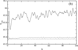
Figure 1: Center of the atomic density distribution $x_{cm}=\sum_{j}|z_{j}|^{2}j$, as a function of the rescaled time $s=t\hbar/U$ (both dimensionless). (a) shows the regular oscillations of the center of the atomic density distribution of a BEC in a harmonic trap obtained by numeric integration of Eqs. (5). (b) shows the same quantity obtained by numerical integration of Eqs. (16) with $\tau=\pi/10$ (continuous), $\pi/4$ (dashed), and $\pi/2$ (dotted) lines.

It is worth noting that, in the present case, the dynamical variables $z_{j},z^{*}_{\ell}$ are related to the expectation values of the boson operators in a more complicated form than in the Glauber CS case. In fact we have $\,{}_{v}\langle z_{j}|a_{j}|z_{j}\rangle_{v}$, = $z_{j}e^{-iu_{1}}\exp[|z_{j}|^{2}(e^{-i2u_{1}}-1)]$. Despite that, the $|z_{j}|^{2}$ still count the number of atoms in each site $j$, see the fourth of Eqs. (13).

IV Numerical simulations

We have numerically integrated Eqs. (5) and (16) on a lattice of $256$ sites, with the initial conditions (13) with the $z_{j}$ given by (6), and for the values of $u_{1}$ corresponding to the waiting times $\tau=\pi/10,\pi/4,\pi/2$. For a BEC in an OL with $T/(2UN)\approx 0.01$, in a harmonic trap with $\lambda_{j}/(2U)=\alpha(j-128)^{2}$ and $\alpha=0.01$, the standard equations of motion (5) imply a superfluid dynamics . This is shown in Fig. 1 (a), where we plot the regular oscillations of the center of the atomic density distribution along the chain. These oscillations have been triggered by displacing the condensates respect to the harmonic trap center, as in the experiment of Ref. Cataliotti_Science293 . On the contrary, once $\tau\neq 0$, the nonstandard equations of motion (16), with the same initial conditions, entail insulator (dissipative) dynamics for the system. This is clearly shown in Fig. 1 (b), where we plot the motion of the system’s center of atomic density distribution for $\tau=\pi/10$ (continuous line), $\pi/4$ (dashed line), and $\pi/2$ (dotted line).

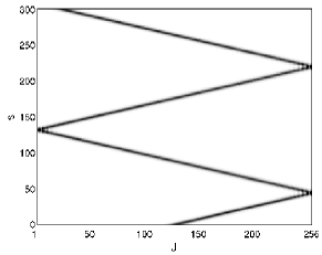
Figure 2: Breather excitation obtained by numeric integration of Eqs. (5) with a Gaussian initial profile. The breather travels along the chain and bounces at the lattice ends. After any bounce, the breather is reconstructed.

We also have performed numerical simulations of Eqs. (5) and (16) by choosing initial conditions in the form of wave packets of Gaussian profile $z^{0}_{j}=\sqrt{k}\exp\{-(j-x)^{2}/\sigma^{2}+ip(j-x)\}$, where $x=128$ is the initial center of the Gaussian, $p=3\pi/4$ is the initial center of mass momenta, $\sigma=10$ is the width of the Gaussian profile, and $k=[\sum_{j}exp(-(j-x)^{2}/(2\sigma^{2}))]^{-1}$.

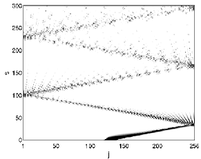
Figure 3: Excitation obtained by numeric integration of Eqs. (16) with the same initial condition as in Fig. 2. The value of the waiting time is $\tau=\pi/2$. This excitation is completely destroyed after a few bounces at the lattice ends. Thus, in the far-from-equilibrium situation, this excitation loses stability and it seems to behave like the states of the diffusion regime that has been identified in Trombettoni_PRL86 .

The dynamics of these profiles have been numerically and analytically studied in Ref. Trombettoni_PRL86 , where a dynamical stability phase diagram for these states was derived. Therein, and also here, the theoretical configuration where the harmonic trapping is off was considered, and the dynamics takes place on a finite lattice endowed with reflecting boundary conditions. Thus, we have performed simulations in the same conditions and we have chosen the combination of the dynamical parameters $T/(2UN)=4.17$, which corresponds to the region of the phase diagram of Ref. Trombettoni_PRL86 where (stable) breather excitations were identified. In Fig. 2 we report the two-dimensional contour plot obtained by numeric integration of (5) with this Gaussian initial condition. In Fig. 2 is clear that the breather structure is maintained when the traveling excitation is reflected at the lattice boundaries. Figure 3 shows the same quantity obtained by integration of Eqs. (16) with the same initial condition as in Fig. 2, and with $\tau=0.5$. Figure 3 clearly shows that the initial excitation, integrated with nonstandard dynamics, pretty soon loses stability, emitting atoms incoherently at any bounce with the lattice boundary.

V Final remarks

In the present paper we have studied how the dynamics of a superfluid is affected by briefly bringing the system into the insulating regime. We have shown that the system is taken to an excited state, described by a superposition of product states of Glauber coherent states at each site, which we have derived. The classical equations of motion ruling its dynamics have been derived. Furthermore, we have shown that these classical equations of motion are inequivalent to the standard discrete nonlinear Schrödinger equations that describe the dynamics of an array of BECs Cataliotti_Science293 in the superfluid regime. By numerically integrating such nonstandard equations with several initial conditions, we have shown that the system loses coherence, becoming insulating.

The simulations we have performed show that the interplay between classical and quantum dynamics leads to loss of the coherence properties of the system. In fact, the brief period in the insulating regimes changes the superfluid wave function, which becomes a superpostion of product states of the site’s coherent states, that is, a product of mean-field states. Each mean-field state has a complicated distribution of phases at each site that results from the intermediate quantum dynamics. This distribution of phases leads to a unique tunneling dynamics described by a complicated hopping term. By a glance at Eqs. (16) one can guess that, as a consequence of this unusual term, the “effective” tunneling rate between close sites in the case of Eqs. (16) becomes site (population) and time dependent. For this reason the system loses coherence.

It is also worth emphasizing that the nonadiabatic procedure we have described in the present paper can straightforwardly be realized in a real experiment similar to those of Refs. Orzel_Science291 ; SF-Diss . Therefore, by displacing the contensates with respect to the harmonic trap, as done in the experiment of Ref. Cataliotti_Science293 , and by observing the oscillations of the center of the atomic density distribution, the effects of the nonstandard dynamics can be directly observed.

- (1) O. Mandel, et al., Nature, 425 937 (2003).
- (2) O. Mandel, et al., Phys. Rev. Lett. 91, 010407 (2003).
- (3) S. Burger, et al., Phys. Rev. Lett. 86, 4447 (2001).
- (4) M. Greiner et al., Nature, 419 51 (2002).
- (5) A. Sinatra and Y. Castin, Eur. Phys. J. D 8, 319 (2002).
- (6) F. S. Cataliotti, et al., Science 293, 843 (2001).
- (7) A. Öttl, et al., Phys. Rev. Lett. 95, 090404 (2005).
- (8) M. Greiner, et al., Nature 415, 39 (2002).
- (9) E. Altman and A. Auerbach, Phys. Rev. Lett. 89, 250404 (2002).
- (10) E. Altman, et al., Phys. Rev. Lett. 95, 020402 (2005).
- (11) P. Buonsante, R. Franzosi and V. Penna, J. Phys. B, 37, s195 (2004).
- (12) C. Orzel, et al., Science 291, 2386 (2001).
- (13) T. Kinoshita, T. Wenger, and D. S. Weiss, Science 305, 1125 (2004).
- (14) D. Jaksch, et al., Phys. Rev. Lett. 81, 3108 (1998).
- (15) C. Menotti, et al., New J. Phys. 5, 112 (2003).
- (16) W. Zwerger, J. Optics B, 5 S9-S16 (2003).
- (17) W.M. Zhang, D.H. Feng, and R. Gilmore, Rev. Mod. Phys. 62, 867 (1990); L. Amico and V. Penna, Phys. Rev. Lett. 80, 2189 (1998); L. Amico and V. Penna, Phys. Rev. B 62, 1224 (2000); A. Montorsi and V. Penna, Phys. Rev. B 55, 8226 (1999).
- (18) A. Trombettoni and A. Smerzi, Phys. Rev. Lett. 86, 2353 (2001).
- (19) S. F. Cataliotti, et al., New J. Phys. 5, 71 (2003).