Generation interval contraction and epidemic data analysis

Abstract

The generation interval is the time between the infection time of an infected person and the infection time of his or her infector.  Probability density functions for generation intervals have been an important input for epidemic models and epidemic data analysis.  In this paper, we specify a general stochastic SIR epidemic model and prove that the mean generation interval decreases when susceptible persons are at risk of infectious contact from multiple sources.  The intuition behind this is that when a susceptible person has multiple potential infectors, there is a “race” to infect him or her in which only the first infectious contact leads to infection.  In an epidemic, the mean generation interval contracts as the prevalence of infection increases.  We call this global competition among potential infectors.  When there is rapid transmission within clusters of contacts, generation interval contraction can be caused by a high local prevalence of infection even when the global prevalence is low.  We call this local competition among potential infectors.  Using simulations, we illustrate both types of competition.  Finally, we show that hazards of infectious contact can be used instead of generation intervals to estimate the time course of the effective reproductive number in an epidemic.  This approach leads naturally to partial likelihoods for epidemic data that are very similar to those that arise in survival analysis, opening a promising avenue of methodological research in infectious disease epidemiology.

1 Introduction

In infectious disease epidemiology, the serial interval is the difference between the symptom onset time of an infected person and the symptom onset time of his or her infector [1].  This is sometimes called the “generation interval.”  However, we find it more useful to adopt the terminology of Svensson [2] and define the generation interval as the difference between the infection time of an infected person and the infection time of his or her infector.  By these definitions, the serial interval is observable while the generation interval usually is not.  We define infectious contact from $i$ to $j$ to be a contact that is sufficient to infect $j$ if $i$ is infectious and $j$ is susceptible, and we define a potential infector of person $i$ to be an infectious person who has positive probability of making infectious contact with $i$.  Finally, we use the term hazard rather than force of infection to highlight the similarities between epidemic data analysis and survival analysis.

The generation interval has been an important input for epidemic models used to investigate the transmission and control of SARS [3, 4] and pandemic influenza [5, 6].  More recently, generation interval distributions have been used to calculate the incubation period distribution of SARS [7] and to estimate $R_{0}$ from the exponential growth rate at the beginning of an epidemic [8].  It is generally assumed that the generation interval distribution is characteristic of an infectious disease.  In this paper, we show that this is not true.  Instead, the expected generation interval decreases as the number of potential infectors of susceptibles increases.  During an epidemic, generation intervals tend to contract as the prevalence of infection increases.  This effect was described by Svensson [2] for an SIR model with homogeneous mixing.  In this paper, we extend this result to all time-homogeneous stochastic SIR models.

A simple thought experiment illustrates the intuition behind our main result.  Imagine a susceptible person $j$ in a room.  Place $m$ other persons in the room and infect them all at time $t=0$.  For simplicity, assume that infectious contact from $i$ to $j$ occurs with probability one, $i=1,...,m$.  Let $t_{ij}$ be a continuous nonnegative random variable denoting the first time at which $i$ makes infectious contact with $j$.  Person $j$ is infected at time $t_{j}=\min(t_{1j},...,t_{mj})$.  Since all infectious persons were infected at time zero, $t_{j}$ is the generation interval.  If we repeat the experiment with larger and larger $m$, the expected value of $\min(t_{1j},...,t_{mj})$ will decrease.

When a susceptible person is at risk of infectious contact from multiple sources, there is a “race” to infect him or her in which only the first infectious contact leads to infection.  Generation interval contraction is an example of a well-known phenomenon in epidemiology: The expected time to an outcome, given that the outcome occurs, decreases in the presence of competing risks.  In our thought experiment, the outcome is the infection of $j$ by a given $i$ and the competing risks are infectious contacts from all sources other than $i$.

Adapting our thought experiment slightly, we see that the contraction of the generation interval is a consequence of the fact that the hazard of infection for $j$ increases as the number of potential infectors increases.  Let $\lambda(t)$ be the hazard of infectious contact from any potential infector to $j$ at time $t$ and let $E[t_{j}|m]$ be the expected infection time of $j$ given $m$ potential infectors.  Then

$$E[t_{j}|m] =\int_{0}^{\infty}e^{-m\lambda(t)}dt$$

$$>\int_{0}^{\infty}e^{-(m+1)\lambda(t)}dt=E[t_{j}|m+1],$$

so the expected generation interval decreases as the number of potential infectors increases.  A hazard of infection that increases with the number of potential infectors is a defining feature of most epidemic models, so generation interval contraction is a very general phenomenon.  We note that a very similar phenomenon occurs in endemic diseases, where increased force of infection results in a decreased average age at first infection [9].

The rest of the paper is organized as follows: In Section 2, we describe a general stochastic SIR epidemic model.  In Section 3, we use this model to show that the mean generation interval decreases as the number of potential infectors increases.  As a corollary, we find that the mean serial interval also decreases.  In Section 4, we consider the role of the population contact structure in generation interval contraction and illustrate the effects of global and local competition among potential infectors with simulations.  In Section 5, we argue that hazards of infectious contact should be used instead of generation or serial interval distributions in the analysis of epidemic data.  Section 6 summarizes our main results and conclusions.

2 General stochastic SIR model

We start with a very general stochastic ”Susceptible-Infectious-Removed” (SIR) epidemic model.  This model includes fully-mixed and network-based models as special cases, and it has been used previously to define a mapping from the final outcomes of stochastic SIR models to the components of semi-directed random networks [10, 11].

Each person $i$ is infected at his or her infection time $t_{i}$, with $t_{i}=\infty$ if $i$ is never infected.  Person $i$ recovers from infectiousness or dies at time $t_{i}+r_{i}$, where the recovery period $r_{i}$ is a positive random variable with the cumulative distribution function (cdf) $F_{i}(r)$.  The recovery period $r_{i}$ may be the sum of a latent period, during which $i$ is infected but not infectious, and an infectious period, during which $i$ can transmit infection.  We assume that all infected persons have a finite recovery period.  If person $i$ is never infected, let $r_{i}=\infty$.  Let Sus$(t)=\{i:t_{i}>t\}$ be the set of susceptibles at time $t$.

When person $i$ is infected, he or she makes infectious contact with person $j$ after an infectious contact interval $\tau_{ij}$.  Each $\tau_{ij}$ is a positive random variable with cdf $F_{ij}(\tau|r_{i})$ and survival function $S_{ij}(\tau|r_{i})=1-F_{ij}(\tau|r_{i})$.  Let $\tau_{ij}=\infty$ if person $i$ never makes infectious contact with person $j$, so the infectious contact interval distribution may have probability mass at $\infty$.  Define

$$S_{ij}(\infty|r_{i})=\lim_{\tau\rightarrow\infty}S_{ij}(\tau|r_{i}),$$

which is the conditional probability that $i$ never makes infectious contact with $j$ given $r_{i}$.  Since a person cannot transmit disease before being infected or after recovering from infectiousness, $S_{ij}(\tau|r_{i})=1$ for all $\tau\leq 0$ and $S_{ij}(\tau|r_{i})=S_{ij}(\infty|r_{i})$ for all $\tau\geq r_{i}$.  Since a person cannot infect himself (or herself), $\tau_{ii}=\infty$ with probability one and $S_{ii}(\tau|r_{i})=1$ for all $\tau$.

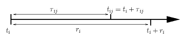
Figure 1: Schematic diagram of variables in the general stochastic SIR model for the ordered pair $ij$. Recall that $t_{j}\leq t_{ij}$. As discussed in Section 3.2, person $i$ develops symptoms at time $t_{i}^{\mathrm{sym}}=t_{i}+q_{i}$, where $q_{i}$ is the incubation period.

The infectious contact time $t_{ij}=t_{i}+\tau_{ij}$ is the time at which person $i$ makes infectious contact with person $j$.  If person $j$ is susceptible at time $t_{ij}$, then $i$ infects $j$ and $t_{j}=t_{ij}$.  If $t_{ij}<\infty$, then $t_{j}\leq t_{ij}$ because person $j$ avoids infection at time $t_{ij}$ only if he or she has already been infected.  If person $i$ never makes infectious contact with person $j$, then $t_{ij}=\infty$ because $\tau_{ij}=\infty$.  Figure 1 shows a schematic diagram of the relationships among $r_{i}$, $\tau_{ij}$, and $t_{ij}$.

The importation time $t_{0i}$ of person $i$ is the earliest time at which he or she receives infectious contact from outside the population.  The importation time vector $\mathbf{t}_{0}=(t_{01},...,t_{0n})$.

We assume that each infected person has a unique infector.  Following [4], we let $v_{i}$ represent the index of the person who infected person $i$, with $v_{i}=0$ for imported infections and $v_{i}=\infty$ if $i$ is never infected.  If tied infectious contact times have nonzero probability, then $v_{i}$ can be chosen from all $j$ such that $t_{ji}=t_{i}<\infty$.

2.1 Epidemics

Let $t_{(1)}\leq t_{(2)}\leq...\leq t_{(m)}$ be the order statistics of all $t_{1},...,t_{n}$ less than infinity, and let $(k)$ be the index of the $k^{\text{th}}$ person infected.  Before the epidemic begins, an importation time vector $\mathbf{t}_{0}$ is chosen.  The epidemic begins at time $t_{(1)}=\min_{i}(t_{0i})$.  Person $(1)$ is assigned a recovery time $r_{(1)}$.  Every person $j\in\,$Sus$(t_{(1)})$ is assigned an infectious contact time $t_{(1)j}=t_{(1)}+\tau_{(1)j}$.  The second infection occurs at $t_{(2)}=\min_{j\in\text{Sus}(t_{(1)})}\min(t_{0j},t_{(1)j})$, which is the first infectious contact time after $t_{(1)}$.  Person $(2)$ is assigned a infectious period $r_{(2)}$.  After $k$ infections, the next infection occurs at $t_{(k+1)}=\min_{j\in\text{Sus}(t_{(k)})}\min(t_{0j},t_{(1)j},...,t_{(k)j})$.  The epidemic stops after $m$ infections if and only if $t_{(m+1)}=\infty$.

3 Generation interval contraction

In this section, we show that the mean infectious contact interval $\tau_{ij}$ given that $i$ infects $j$ is shorter than the mean infectious contact interval given that $i$ makes infectious contact with $j$.  In the notation from the previous section,

$$E[\tau_{ij}|v_{j}=i]\leq E[\tau_{ij}|\tau_{ij}<\infty]$$

(note that $v_{j}=i$ implies $\tau_{ij}<\infty$ but not vice versa).  In general, this inequality is strict when $j$ is at risk of infectious contact from any source other than $i$.  This inequality implies the contraction of generation and serial intervals during an epidemic.  For background on the probability theory used in this section, please see Ref. [12] or any other probability text.

Lemma 1

$E[\tau_{ij}|v_{j}=i]\leq E[\tau_{ij}|\tau_{ij}<\infty].$

Proof. We first show that $E[\tau_{ij}|r_{i},\tau_{ij}<\infty]\leq E[\tau_{ij}|r_{i},v_{j}=i]$ and then use the law of iterated expectation.  If person $i$ was infected at time $t_{i}$ and has recovery period $r_{i}$, then the probability that $\tau_{ij}<\infty$ is $F_{ij}(\infty|r_{i})=1-S_{ij}(\infty|r_{i})$.  Let

$$F_{ij}^{\ast}(\tau|r_{i})=\frac{F_{ij}(\tau|r_{i})}{F_{ij}(\infty|r_{i})}$$

be the conditional cdf of $\tau_{ij}$ given $r_{i}$ and $\tau_{ij}<\infty$.  Then

$$E[\tau_{ij}|r_{i},\tau_{ij}<\infty]=\int_{0}^{r_{i}}\tau dF_{ij}^{\ast}(\tau|r_{i}).$$ (1)

If person $j$ is susceptible at time $t_{i}$ and $\tau_{ij}<\infty$, then $v_{j}=i$ if and only if $j$ escapes infectious contact from all other infectious people during the time interval $(t_{i},t_{i}+\tau_{ij})$.  Let $S_{\ast j}(t_{i}+\tau)$ be the probability that $j$ escapes infectious contact from all sources other than $i$ in the interval $(t_{i},t_{i}+\tau)$.  Given $r_{i}$ and $\tau_{ij}<\infty$, the conditional probability density for an infectious contact from $i$ to $j$ at time $t_{i}+\tau$ that leads to the infection of $j$ is proportional to

$$S_{\ast j}(t_{i}+\tau)dF_{ij}^{\ast}(\tau|r_{i}).$$

If we let

$$\psi=\int_{0}^{r_{i}}S_{\ast j}(t_{i}+\tau)dF_{ij}^{\ast}(\tau|r_{i}),$$

then

$$E[\tau_{ij}|r_{i},v_{j}=i]=\int_{0}^{r_{i}}\tau\frac{S_{\ast j}(t_{i}+\tau)}{\psi}dF_{ij}^{\ast}(\tau|r_{i}).$$

Since $S_{\ast j}(t_{i}+\tau_{ij})$ is a monotonically decreasing function of $\tau_{ij}$,

$$E[\tau_{ij}|r_{i},v_{j}=i]-E[\tau_{ij}|r_{i},\tau_{ij}<\infty]=~{} E[\tau_{ij}\frac{S_{\ast j}(t_{i}+\tau_{ij})}{\psi}|r_{i},\tau_{ij}<\infty]$$

$$-E[\tau_{ij}|r_{i},\tau_{ij}<\infty]E[\frac{S_{\ast j}(t_{i}+\tau_{ij})}{\psi}|r_{i},\tau_{ij}<\infty]$$

$$=~{} \text{Cov}(\tau_{ij},\frac{S_{\ast j}(t_{i}+\tau_{ij})}{\psi}|r_{i},\tau_{ij}<\infty)$$

$$\leq ~{}0.$$

Therefore,

$$E[\tau_{ij}|r_{i},v_{j}=i]\leq E[\tau_{ij}|r_{i},\tau_{ij}<\infty].$$ (2)

Since the same inequality holds for all $r_{i}$,

$$E[\tau_{ij}|v_{j}=i] =E[E[\tau_{ij}|r_{i},v_{j}=i]]$$

$$\leq E[E[\tau_{ij}|r_{i},\tau_{ij}<\infty]]=E[\tau_{ij}|\tau_{ij}<\infty]$$ (3)

by the law of iterated expectation.    

Equality holds in equation (2) if and only if $\tau_{ij}$ and $S_{\ast j}(t_{i}+\tau_{ij})$ have covariance zero given $r_{i}$ and $\tau_{ij}<\infty$.  Since $S_{\ast j}(t_{i}+\tau_{ij})$ is a monotonically decreasing function of $\tau_{ij}$, this will occur if and only if $\tau_{ij}$ or $S_{\ast j}(t_{i}+\tau_{ij})$ is constant given $r_{i}$ and $\tau_{ij}<\infty$.  Equality holds in equation (3) if and only if equality holds in (2) with probability one in $r_{i}$.   If $\tau_{ij}$ is constant, then clearly $S_{\ast j}(t_{i}+\tau_{ij})$ is constant and their covariance is zero.  If $j$ is not at risk of infectious contact from any source other than $i$, then $S_{\ast j}(t_{i}+\tau_{ij})$ will be constant even when $\tau_{ij}$ is not.  In the thought experiment from the Introduction, the expected infection time of the susceptible $j$ would remain constant in the following two scenarios: (i) all infectious persons make infectious contact with $j$ at a fixed time $t_{0}$, or  (ii) $j$ is only at risk of infectious contact from a single person.  Scenario (i) corresponds to a constant $\tau_{ij}$ and scenario (ii) corresponds to a constant $S_{\ast j}(t_{i}+\tau_{ij})$.

The expected generation interval from $i$ to $j$ given $v_{j}=i$ will be shortest when the risk of infectious contact to $j$ from sources other than $i$ is greatest.  More specifically,

$$E[\tau_{ij}|r_{i},v_{j}=i]-E[\tau_{ij}|r_{i},\tau_{ij}<\infty]$$

will be minimized when $S_{\ast j}(t_{i}+\tau_{ij})$ decreases fastest in $\tau_{ij}$.  In general, the risk of infectious contact from other sources will be greatest when the prevalence of infection is highest, so we expect the greatest contraction of the serial interval during an epidemic to coincide with the peak prevalence of infection.

In general, we expect to see the following pattern over the course of an epidemic: The mean generation interval decreases as the prevalence of infection increases, reaches a minimum as the prevalence of infection peaks, and increases again as the prevalence of infection decreases.

3.1 Types of generation intervals

In [2], Svennson discussed two types of generation intervals that are consistent with the verbal definition given in the Introduction.  $T_{p}$ ($p$ for “primary”) denotes $\tau_{ij}$ where $i$ is chosen at random from all persons who infect at least one other person and $j$ is chosen randomly from the set of persons $i$ infects.  $T_{s}$ ($s$ for “secondary”) denotes $\tau_{ij}$ where $j$ is chosen at random from all persons infected from within the population and $i=v_{j}$.  $T_{p}$ and $T_{s}$ differ only in the sampling procedure used to obtain the ordered pair $ij$; $T_{p}$ samples primary cases (infectors) at random while $T_{s}$ samples secondary cases at random.  Equation (3) implies that both $E[T_{p}]$ and $E[T_{s}]$ decrease when susceptible persons are at risk of infectious contact from multiple sources.  This contraction occurs because the definitions of $T_{p}$ and $T_{s}$ include only $\tau_{ij}$ such that $i$ actually infected $j$.

3.2 Serial interval contraction

In an epidemic, infection times are generally unobserved.  Instead, symptom onset times are observed.  Recall that the time between the onset of symptoms in an infected person and the onset of symptoms in his or her infector is called the serial interval.  Contraction of the mean generation interval implies contraction of the mean serial interval as well.  The incubation period is the time from infection to the onset of symptoms [1].  Let $q_{i}$ be the incubation period in person $i$, and let $t_{i}^{\text{sym}}=t_{i}+q_{i}$ be the time of his or her onset of symptoms.  If $v_{j}=i$, then the serial interval associated with person $j$ is

$$t_{j}^{\text{sym}}-t_{i}^{\text{sym}}=\tau_{ij}+q_{j}-q_{i}.$$

Therefore,

$$E[t_{j}^{\text{sym}}-t_{i}^{\text{sym}}|v_{j}=i] =E[\tau_{ij}|v_{j}=i]+E[q_{j}]-E[q_{i}]$$

$$\leq E[\tau_{ij}|\tau_{ij}<\infty]+E[q_{j}]-E[q_{i}],$$

with strict inequality whenever strict inequality holds for the corresponding generation interval.  Over the course of an epidemic, we expect the mean serial interval to follow a pattern very similar to that of the mean generation interval.

4 Simulations

We refer to the “race” to infect a susceptible person as competition among potential infectors.  In this section, we illustrate two types of competition among potential infectors: Global competition among potential infectors results from a high global prevalence of infection.  Local competition among potential infectors results from rapid transmission within clusters of contacts, which causes susceptibles to be at risk of infectious contact from multiple sources within their clusters even if the global prevalence of infection is low.  In real epidemics, the prevalence of infection is usually low but there is clustering of contacts within households, hospital wards, schools, and other settings.

In this section, we use simulations to illustrate generation interval contraction under global and local competition among potential infectors.  Each simulation is a single realization of a stochastic SIR model in a population of $10,000$.  We keep track of the infection times of the primary and secondary case in each infector/infectee pair and the prevalence of infection at the infection time of the secondary case, which is a proxy for the amount of competition to infect the secondary case.  We then calculate a smoothed mean of the generation interval as a function of the infection time of the primary case in each pair.  Another valid approach would be to calculate the smoothed means from the results of many simulations.  We did not take this approach for the following reasons: (i) Because of variation in the time course of different realizations of the same stochastic SIR model, many simulations would be required to obtain a curve that reliably approximates the asymptotic limit. (ii) The smoothed mean over many simulations would show a pattern similar to that obtained in any single simulation.  (iii) Generation interval contraction was proven in Section 3, so the simulations are intended primarily as illustrations.

All simulations were implemented in Mathematica 5.0.0.0 [©1988-2003 Wolfram Research, Inc.].  All data analysis was done using Intercooled Stata 9.2 [© 1985-2007 StataCorp LP]  All smoothed means are running means with a bandwidth of $0.8$ (the default for the Stata command lowess with the option mean).  Similar results were obtained for larger and smaller bandwidths.

4.1 Global competition

To illustrate global competition among potential infectors, we use a fully-mixed model with population size $n=10,000$ and basic reproductive number $R_{0}$.  The infectious period is fixed, with $r_{i}=1$ with probability one for all $i$.  The infectious contact intervals $\tau_{ij}$ have an exponential distribution with hazard $R_{0}(n-1)^{-1}$ truncated at $r_{i}$, so $S_{ij}(\tau|r_{i})=e^{-R_{0}(n-1)^{-1}\tau}$ when $0<\tau<1$ and $\tau_{ij}=\infty$ with probability $e^{-R_{0}(n-1)^{-1}}$.  The epidemic starts with a single imported infection and no other imported infections occur.

From equation (1), the mean infectious contact interval given that contact occurs is

$$E[\tau_{ij}|\tau_{ij}<\infty]=\int_{0}^{1}\frac{e^{-R_{0}\tau(n-1)^{-1}}-e^{-R_{0}(n-1)^{-1}}}{1-e^{-R_{0}(n-1)^{-1}}}d\tau$$

For $n=10,000$, Table 1 shows this expected value at each $R_{0}$.  For all $R_{0}$, $E[\tau_{ij}|\tau_{ij}<\infty]\approx.5$.

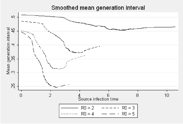
Figure 2: The smoothed mean generation interval as a function the source infection time for $R_{0}=2,3,4,5$.  There is a clear tendency to contract, with greater contraction for higher $R_{0}$.

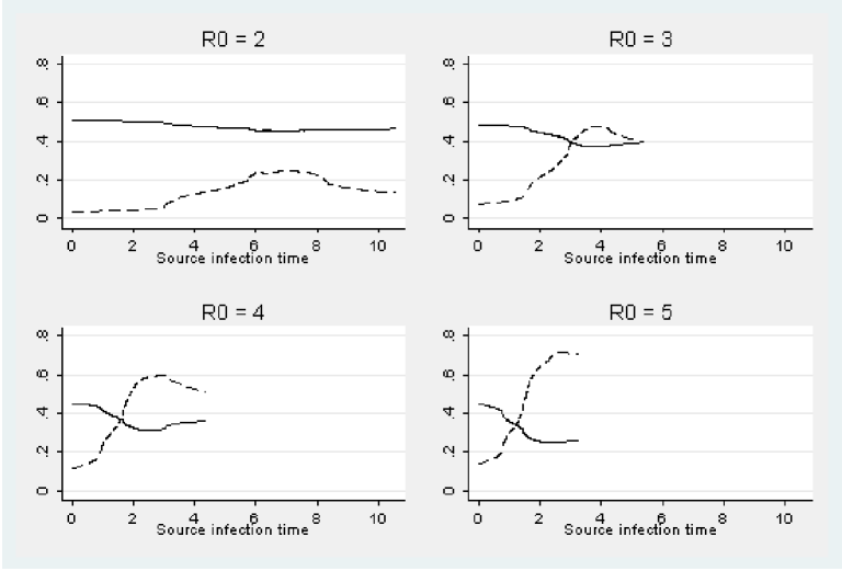
Figure 3: The smoothed mean generation interval (solid lines) and prevalence (dotted lines) as a function of the source infection time for $R_{0}=2,3,4,5$.  In all cases, the greatest contraction of the serial interval coincides with the peak prevalence of infection (i.e., the greatest competition among potential infectors).

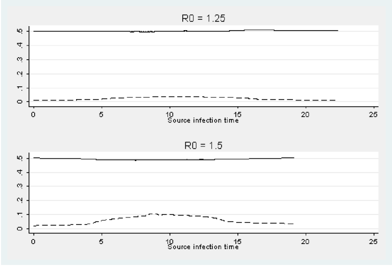
Figure 4: The smoothed mean generation intervals (solid lines) and prevalence (dotted lines) as a function of the source infection time for $R_{0}=1.25$ and $1.50$.  For $R_{0}$ near one, the mean generation interval stays relatively constant.

This model was run once at $R_{0}=1.25$, $1.5$, $2$, $3$, $4$, $5$, and $10$.  For each simulation, we recorded $t_{i}$, $v_{i}$, $t_{v_{i}}$, and the prevalence of infection at time $t_{i}$ in each infector/infectee pair.  Figure 2 shows smoothed mean curves for the generation interval versus the source infection time for $R_{0}=2,3,4,5$.  There is a clear tendency for the mean generation interval to contract, with greater contraction at higher $R_{0}$.  Figure 3 shows smoothed mean curves for the generation interval and the prevalence of infection versus the source infection time at each $R_{0}$; in each case, the greatest contraction of the serial interval coincides with the peak prevalence of infection (i.e., the greatest competition among potential infectors).  Figure 4 shows the same curves for $R_{0}=1.25$ and $1.50$; in these cases, the generation interval stays relatively constant.  These results are exactly in line with the argument of Section 3.

4.2 Local competition

To illustrate local competition among potential infectors, we grouped a population of $n=9,000$ individuals into clusters of size $k$.  As before, the infectious period is fixed at $r_{i}=1$ for all $i$.  When $i$ and $j$ are in the same cluster, the infectious contact interval $\tau_{ij}$ has an exponential distribution with hazard $\lambda_{\text{within}}$ truncated at $r_{i}$, so $S_{ij}(\tau|r_{i})=e^{-\lambda_{\text{within}}\tau}$ when $0<\tau<1$ and $\tau_{ij}=\infty$ with probability $e^{-\lambda_{\text{within}}}$.  When $i$ and $j$ are in different clusters, $\tau_{ij}$ has an exponential distribution with hazard $\lambda_{\text{between}}$ truncated at $r_{i}$, so $S_{ij}(\tau|r_{i})=e^{-\lambda_{\text{between}}\tau}$ when $0<\tau<1$ and $\tau_{ij}=\infty$ with probability $e^{-\lambda_{\text{between}}}$.

We fixed the hazard of infectious contact between individuals in the same cluster at $\lambda_{\text{within}}=.4$.  We tuned the hazard of infectious contact between individuals in different clusters to obtain $R$ mean infectious contacts by infectious individuals; specifically,

$$\lambda_{\text{between}}=\frac{R-(k-1)(1-e^{-.4})}{n-k}.$$

We chose $\lambda_{\text{within}}=.4$ to obtain rapid transmission within clusters while retaining sufficient transmission between clusters to sustain an epidemic.  Note that when $k>R(1-e^{-.4})^{-1}+1$, we get the implausible result that $\lambda_{\text{between}}<0$.  Clearly, $R$ and $k$ must be chosen so that an infectious person makes an average of $R$ or fewer infectious contacts within his or her cluster, which guarantees that $\lambda_{\text{between}}\geq 0$.

At a given $R$, the mean infectious contact interval given that infectious contact occurs depends on the cluster size.  If the entire population is infectious and the cluster size is $k$, then a given individual will receive an average of $R$ infectious contacts, of which $(k-1)(1-e^{-.4})$ come from within his or her cluster.  The mean infectious contact interval for within-cluster contacts is

$$\frac{1}{1-e^{-.4}}\int_{0}^{1}.4\tau e^{-.4\tau}d\tau,$$

and the mean infectious contact interval for between-cluster contacts is approximately $.5$ (as in the models for global competition).  Therefore, the mean infectious contact interval given that contact occurs and the cluster size is $k$ is

$$E[\tau_{ij}|\tau_{ij}<\infty,k]\approx(1-\frac{(k-1)(1-e^{-.4})}{R}).5+\frac{(k-1)}{R}\int_{0}^{1}.4\tau e^{-.4\tau}d\tau.$$

To compare generation interval contraction for different cluster sizes, we calculated scaled generation intervals by dividing the observed generation intervals at each cluster size by $E[\tau_{ij}|\tau_{ij}<\infty,k]$.  If the mean generation interval remained constant, we would expect the mean scaled generation interval to be approximately one throughout an epidemic.

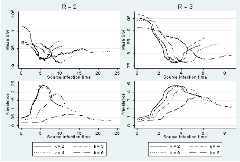
Figure 5: The smoothed mean scaled generation interval (SGI) and prevalence as a function of the source infection time for $R=2$ and $R=3$.  With increasing cluster size, the degree of generation interval contraction is roughly the same even though the peak prevalence of infection is lower.

For $R=2$, we ran the model with cluster sizes of $1$ through $6$.  For $R=3$, we ran the model with cluster sizes of $2$ through $8$.  For each simulation, we recorded $t_{i}$, $v_{i}$, $t_{v_{i}}$, and the prevalence of infection at time $t_{i}$ in each infector/infectee pair.  Figure 5 shows smoothed mean curves for the generation interval and prevalence versus the source infection time for several cluster sizes at each $R$.  As before, there is a clear tendency of the mean generation interval to contract.  The degree of contraction is roughly the same for all cluster sizes, but this contraction is maintained at a lower global prevalence of infection in models with larger cluster sizes.  Similar results were obtained for cluster sizes not shown.  Again, these results are exactly in line with the argument of Section 3.

5 Consequences for estimation

The effect of generation interval contraction on parameter estimates obtained from models that assume a constant generation or serial interval distribution is difficult to assess.  The assumption of a constant serial or generation interval distribution may be reasonable in the early stages of an epidemic with little clustering of contacts, in an epidemic with $R_{0}$ near one, or in an endemic situation.  However, this ignores the more fundamental issue that estimates of these distributions are obtained from transmission events where the infector/infectee pairs are known (often because of transmission from a known patient within a household or hospital ward).  Even in the early stages of an epidemic, the generation interval distribution in these settings may differ substantially from the generation interval distribution for transmission in the general population.

In this section, we argue that hazards of infectious contact can be used instead of generation or serial intervals in the analysis of epidemic data.  As an example, we look at the estimator of $R(t)$ (the effective reproductive number at time $t$) derived by Wallinga and Teunis [4] and applied to data on the SARS outbreaks in Hong Kong, Vietnam, Singapore, and Canada in 2003.  In their paper, the available data was the “epidemic curve” $\mathbf{t}=(t_{(1)},...,t_{(m)})$, where $t_{(i)}$ is the infection time of the $i^{\text{th}}$ person infected.  They assume a probability density function (pdf) $w(\tau|\mathbf{\theta})$ for the serial interval given a vector $\mathbf{\theta}$ of parameters (note that this parameter vector applies to the population, not to individuals).  The infector of person $(i)$ is denoted by $v_{(i)}$, with $v_{(i)}=0$ for imported infections.  The “infection network” is a vector $\mathbf{v}=(v_{(1)},...,v_{(m)})$ specifying the source of infection for each infected person.  With these assumptions, the likelihood of $\mathbf{v}$ and $\mathbf{\theta}$ given $\mathbf{t}$ is

$$L(\mathbf{v},\mathbf{\theta}|\mathbf{t})=\prod_{i:v_{(i)}\neq 0}w(t_{(i)}-t_{v_{(i)}}|\mathbf{\theta}).$$

The sum of this likelihood over the set $V$ of all infection networks consistent with the epidemic curve $\mathbf{t}$ is

$$L(\mathbf{\theta}|\mathbf{t})=\prod_{i:v_{(i)}\neq 0}\sum_{j\neq i}w(t_{i}-t_{j}|\mathbf{\theta}).$$

Taking a likelihood ratio, Wallinga and Teunis argue that the relative likelihood that person $k$ was infected by person $j$ is

$$p_{jk}^{(WT)}=\frac{w(t_{k}-t_{j}|\mathbf{\theta})}{\sum_{i\neq k}w(t_{k}-t_{i}|\mathbf{\theta})}.$$ (4)

The number $R_{j}$ of secondary infectious generated by person $j$ is a sum of Bernoulli random variables with expectation

$$E[R_{j}]=\sum_{k=1}^{n}p_{jk}^{(WT)}.$$

An estimate of the effective reproductive number $R(t)$ can be obtained by calculating a smoothed mean for a scatterplot of $(t_{j},E[R_{j}])$.  This analysis is ingenious, but it can be only approximately correct because the distribution of serial intervals varies systematically over the course of an epidemic.

5.1 Hazard-based estimator

A very similar result can be derived by applying the theory of order statistics (see Ref. [12]) to the general stochastic SIR model from Section 2.  Specifically, we use the following results: If $X_{1},...,X_{n}$ are independent non-negative random variables, then their minimum $X_{(1)}$ has the hazard function

$$\lambda_{(1)}(t)=\sum_{i=1}^{n}\lambda_{i}(t).$$

Given that the minimum is $x_{(1)}$, the probability that $X_{j}=x_{(1)}$ (i.e. that the minimum was observed in the $j^{\text{th}}$ random variable) is

$$\frac{\lambda_{j}(x_{(1)})}{\sum_{i=1}^{n}\lambda_{i}(x_{(1)})}.$$

For simplicity, we assume that the infectious contact intervals $\tau_{ij}$ are absolutely continuous random variables.

Let $\lambda_{ij}(\tau|r_{i})$ be the conditional hazard function for $\tau_{ij}$ given $r_{i}$ and let $\lambda_{0i}(t)$ be the hazard function for infectious contact to $i$ from outside the population at time $t$.  Since $\tau_{ij}$ is nonnegative, $\lambda_{ij}(\tau|r_{i})=0$ whenever $\tau<0$.  Let $H(t)$ denote the set of infection times and recovery periods for all $i$ such that $t_{i}\leq t$.  If person $k$ is susceptible at time $t$, his or her total hazard of infection at time $t$ given $H(t)$ is $\sum_{i=0}^{n}\lambda_{ik}(t-t_{i}|r_{i})$, where we let $\lambda_{0k}(t-t_{0}|r_{0})=\lambda_{0k}(t)$ for simplicity of notation.  If an infection occurs in person $k$ at time $t_{k}<\infty$, then the conditional probability that person $j$ infected person $k$ given $H(t_{k})$ is

$$p_{jk}=\frac{\lambda_{jk}(t_{k}-t_{j}|r_{j})}{\sum_{i=0}^{n}\lambda_{ik}(t_{k}-t_{i}|r_{i})},$$ (5)

which is the probability that $t_{jk}=\min(t_{0k},t_{1k},...,t_{nk})$.  This has the same form as equation (4) except that it uses hazards of infectious contact instead of a pdf for the serial interval.  If the hazards of infectious contact in the underlying SIR model do not change over the course of an epidemic, then $p_{jk}$ can be estimated accurately throughout an epidemic.  Unlike the assumption of a stable generation or serial interval distribution, this assumption is unaffected by competition among potential infectors.  The rest of the estimation of $R(t)$ could proceed exactly as in Ref. [4], replacing $p_{jk}^{(WT)}$ with $p_{jk}$.

5.2 Partial likelihood for epidemic data

A partial likelihood for epidemic data can be derived using the same logic as that used to derive $p_{jk}$ in equation (5).  For each person $k$ such that $t_{k}<\infty$, the probability that the failure at time $t_{k}$ occurred in person $k$ given $H(t_{k})$ is

$$\frac{\sum_{i=0}^{n}\lambda_{ik}(t_{k}-t_{i}|r_{i})}{\sum_{j=1}^{n}\sum_{i=0}^{n}\lambda_{ij}(t_{k}-t_{i}|r_{i})},$$ (6)

where the numerator is the hazard of infection (from all sources) in person $k$ at time $t_{k}$ and the denominator is the total hazard of infection for all persons at risk of infection at time $t_{k}$.

If there is a vector of parameters $\mathbf{x}_{ij}$ for each pair $ij$ (which may include individual-level covariates for $i$ and $j$ as well as pairwise covariates for the ordered pair $ij$) and a vector of parameters $\mathbf{\theta}$ such that $\lambda_{ij}(\tau|r_{i})=\lambda(\tau|r_{i},\mathbf{x}_{ij},\mathbf{\theta})$, then a partial likelihood for $\mathbf{\theta}$ can be obtained by multiplying equation (6) over all $m$ observed failure times.  If $(k)$ denotes the index of the $k^{\text{th}}$ person infected, $\mathbf{t}=(t_{1},...,t_{n})$, and $\mathbf{X}=\{\mathbf{x}_{ij}:i,j=1,...,n\}$, then the partial likelihood is

$$L_{p}(\mathbf{\theta}|\mathbf{t},\mathbf{X})=\prod_{k=1}^{m}\frac{\sum_{i=0}^{n}\lambda(t_{(k)}-t_{i}|r_{i},\mathbf{x}_{i(k)},\mathbf{\theta})}{\sum_{j=1}^{n}\sum_{i=0}^{n}\lambda(t_{k}-t_{i}|r_{i},\mathbf{x}_{ij},\mathbf{\theta})}.$$ (7)

This is very similar to partial likelihoods that arise in survival analysis, so many techniques from survival analysis may be adaptable for use in the analysis of epidemic data.

The goal of such methods would be to allow statistical inference about the effects of individual and pairwise covariates on the hazard of infection in ordered pairs of individuals.  In the ordered pair $ij$, the effects of individual covariates for $i$ and $j$ on $\lambda_{ij}(\tau|r_{i})$ would reflect the infectiousness of $i$ and the susceptibility of $j$, respectively.  Pairwise covariates could include such information as whether $i$ and $j$ are in the same household, the distance between their households, whether they are sexual partners, and any other aspects of their relationship to each other thay may affect the hazard of infection from $i$ to $j$.

This approach has several advantages over any approach based on a distribution of generation or serial intervals.  First, it is not necessary to determine who infected whom in any subset of observed infections.  If $v_{j}$ is known for some $j$, this knowledge can be incorporated in the partial likelihood by replacing the term for the failure time of person $j$ in (7) with $p_{v_{j}j}$ from equation (5).  Second, this approach allows the use individual-level and pairwise covariates for inference in a flexible and intuitive way.  The resulting estimated hazard functions have a straightforward interpretation and can be incorporated naturally into a stochastic SIR model.  Third, this approach allows theory and methods from survival analysis to be applied to the analysis of epidemic data.

6 Discussion

Generation and serial interval distributions are not stable characteristics of an infectious disease.  When multiple infectious persons compete to infect a given susceptible person, infection is caused by the first person to make infectious contact.  In Section 3, we showed that the mean infectious contact interval $\tau_{ij}$ given that $i$ actually infected $j$ is less than or equal to the mean $\tau_{ij}$ given $i$ made infectious contact with $j$.  That is,

$$E[\tau_{ij}|v_{j}=i]\leq E[\tau_{ij}|\tau_{ij}<\infty],$$

with strict inequality when $\tau_{ij}$ is non-constant and $j$ is at risk of infectious contact from any source other than $i$ (more precise conditions are given in Section 3).  This result holds for all time-homogeneous stochastic SIR models.

In an epidemic, the mean generation (and serial) intervals contract as the prevalence of infection increases and susceptible persons are at risk of infectious contact from multiple sources.  In the simulations of Section 4, we saw that the degree of contraction increases with $R_{0}$.  For models with clustering of contacts, generation interval contraction can occur even when the global prevalence of infection is low because susceptibles are at risk of infectious contact from multiple sources within their own clusters.  In all of the simulations, the greatest serial interval contraction coincided with the peak prevalence of infection, when the risk of infectious contacts from multiple sources was highest.  The mean generation interval increases again as the epidemic wanes, but this rebound may be small when $R_{0}$ is high.

The reason that generation and serial intervals contract during an epidemic is that their definition applies to pairs of individuals $ij$ such that $i$ actually transmitted infection to $j$.  If we don’t require that an infectious contact leads to the transmission of infection, we are led naturally to the concept of the infectious contact interval, which has a well-defined distribution throughout an epidemic.  Similarly, we can define $R_{0}$ as the mean number of infectious contacts (i.e., finite infectious contact intervals) made by a primary case without reference to a completely susceptible population.  Generation and serial intervals and the effective reproductive number can then be defined in terms of infectious contacts that actually lead to the transmission of infection.  Many fundamental concepts in infectious disease epidemiology can be simplified usefully by defining them in terms of infectious contact rather than infection transmission.

Infectious contact hazards for ordered pairs of individuals can be used for many of the same types of analysis that have been attempted using generation or serial interval distributions.  In Section 5, We derived a hazard-based estimator of $R(t)$ very similar to that developed by Wallinga and Teunis [4].  This derivation led naturally to a partial likelihood for epidemic data very similar to those that arise in survival analysis.  We believe that the adaptation of methods and theory from survival analysis to infectious disease epidemiology will yield flexible and powerful tools for epidemic data analysis.

Acknowledgements: This work was supported by the US National Institutes of Health cooperative agreement 5U01GM076497 ”Models of Infectious Disease Agent Study” (E.K. and M.L.) and Ruth L. Kirchstein National Research Service Award 5T32AI007535 ”Epidemiology of Infectious Diseases and Biodefense” (E.K.).  We also wish to thank Jacco Wallinga and the anonymous reviewers of Mathematical Biosciences for useful comments and suggestions.

Appendix A Figures and tables

$\mathbf{R}_{0}$	$\mathbf{E[\tau}_{ij}|\mathbf{\tau}_{ij}<\infty\mathbf{]}$	$.5-\mathbf{E[\tau}_{ij}|\mathbf{\tau}_{ij}<\infty\mathbf{]}$
$1.25$	$.49999$	$.00001$
$1.5$	$.499988$	$.000012$
$2$	$.499983$	$.000017$
$3$	$.499975$	$.000025$
$4$	$.499967$	$.000033$
$5$	$.499958$	$.000042$

Table 1: Expected infectious contact interval given that infectious contact occurs in the models illustrating global competition among potential infectors. If the generation interval were constant, this would be the mean generation interval throughout an epidemic.

References

- [1] J. Giesecke. Modern Infectious Disease Epidemiology. London: Edward Arnold, 1994.
- [2] Å. Svensson (2007). A note on generation times in epidemic models. Mathematical Biosciences, 208: 300-311.
- [3] M. Lipsitch, T. Cohen, B. Cooper, et al. (2003). Transmission dynamics and control of Severe Acute Respiratory Syndrome. Science, 300: 1966-1970.
- [4] J. Wallinga and P. Teunis (2004). Different epidemic curves for Severe Acute Respiratory Syndrome Reveal Similar Impacts of Control Measures. American Journal of Epidemiology, 160(6): 509-516.
- [5] C.E. Mills, J. Robins, and M. Lipsitch (2004). Transmissibility of 1918 pandemic influenza. Nature 432: 904.
- [6] N.M. Ferguson, D.A.T. Cummings, S. Cauchemez, C. Fraser, S. Riley, A. Meeyai, S. Iamsirithaworn, and D. Burke. Strategies for containing an emerging influenza pandemic in Southeast Asia. Nature 437: 209-214.
- [7] A.Y. Kuk and S. Ma (2005). Estimation of SARS incubation distribution from serial interval data using a convolution likelihood. Statistics in Medicine 24(16): 2525-37.
- [8] J. Wallinga and M. Lipsitch (2007). How generation intervals shape the relationship between growth rates and reproductive numbers. Proceedings of the Royal Society B, 274: 599-604.
- [9] R. M. Anderson and R. M. May. Infectious Diseases of Humans: Dynamics and Control. New York: Oxford University Press, 1991.
- [10] E. Kenah and J. Robins (2007). Second look at the spread of epidemics on networks. Physical Review E 76: 036113.
- [11] E. Kenah and J. Robins (2007). Network-based analysis of stochastic SIR epidemic models with random and proportionate mixing. Journal of Theoretical Biology 249(4): 706-722.
- [12] A. Gut (1995). An Intermediate Course in Probability. New York: Springer-Verlag.