Investigation of electric fields in plasmas under pulsed currents

Abstract

Electric fields in a plasma that conducts a high-current pulse are measured as a function of time and space. The experiment is performed using a coaxial configuration, in which a current rising to 160 kA in 100 ns is conducted through a plasma that prefills the region between two coaxial electrodes. The electric field is determined using laser spectroscopy and line-shape analysis. Plasma doping allows for 3D spatially resolved measurements. The measured peak magnitude and propagation velocity of the electric field is found to match those of the Hall electric field, inferred from the magnetic-field front propagation measured previously.

I Introduction

For a long time, laboratory experiments and observations in space have been stirring up a dispute concerning the mechanisms of the magnetic-field evolution in plasma and the associated plasma dynamics. Estimates of the plasma collisionality in plasma opening switches (POS), for example, indicate that the magnetic field diffusion should be small while the plasma pushing by the magnetic-field pressure should be dominant. However, magnetic-field penetration has been observed in POS experiments Weber , and, moreover, it is found to be significantly faster than expected from diffusion Spitalnik ; PRL ; B-fieldRon ; Dynamics . The magnetic-field penetration was also found to be higher than, or of a comparable velocity to the plasma pushing. In an early experiment Spitalnik a fast magnetic-field penetration into a plasma where the ions are nearly immobile was observed. This was explained by the generation of an electric Hall field based on the electron magnetohydrodynamics theory Kingsep1 ; Gordeev1 ; Fruchtman ; FruchtmanPRA . The relative importance of the two governing processes, i.e., the plasma pushing and the magnetic-field penetration, was further analyzed in a series of additional experiments with different plasma parameters, in which comprehensive measurements of spatial distributions of the magnetic field, of the ion velocity, and of the electron density in the plasma were performed. These detailed measurements, performed in multi-ion species plasma, have revealed that the fast magnetic field penetration into the plasma is accompanied by a specular reflection of the light-ion plasma and a slow pushing of the heavy-ion plasma penetrated by the field B-fieldRon ; Dynamics , resulting in ion-species separation PRL .

The electric field plays a crucial role in the interaction of the magnetic field with the plasma. The electric field transfers energy to the current-carrying plasma through the Joule heating, the electric field that is generated by the space-charge separation due to the magnetic field accelerates the ions, and the (Hall) electric field may induce the magnetic-field penetration into the plasma. However, previous studies of the electric fields in plasmas under application of pulsed currents (e.g., Refs. Weingarten_turbulence ; B-fieldRon ; Dynamics ) lacked the temporal and spatial resolutions and, thus, only provided an averaged view.

In this paper we describe an application of 3D-resolved spectroscopy to investigate the time evolution of electric fields in plasmas under high-current pulses. Our method is based on laser spectroscopy combined with plasma doping by lithium, which allows for electric field measurements from the lithium emission-line shape. In the following sections we first discuss the physics underlying the diagnostic method and the measurements of the initial conditions of the plasma prior to the application of the current. Then, measurements of the electric field in the plasma under a current pulse are described, followed by a discussion on the relation between the measured electric field, the magnetic field, and the plasma dynamics. It is found that the measured electric field magnitude is consistent with the Hall electric field calculated on the basis of the magnetic field and the plasma density measured in a separate study.

II The diagnostic method

The Stark effect has proven to be of a great utility for non-intrusive measurements of the frequency and amplitude of local electric fields in plasmas, as first suggested by Baranger and Mozer Baranger and shortly later experimentally verified by Kunze and Griem Kunze-Griem .

The advantages of the lithium atomic system for electric fields measurements have been previously demonstrated Rebhan-Kunze ; Hildebrandt ; Rebhan . Lithium was employed for measurements of electric fields in dilute plasmas of gas discharges Burrell ; Kawasaki and in the vacuum gap of a high-voltage diode Knyazev . In our experiment, high spatial and temporal resolutions in measuring the electric fields in relatively dense ($\sim 10^{14}~{}cm^{-3}$) plasma are achieved. At such densities, extracting the information from the spectral line-profiles becomes more difficult due to the increased Stark broadening and the faster ionization processes that reduce the neutral lithium line emission.

The E-field diagnostic is based on the analysis of the line-shape of a forbidden transition and its intensity relative to an allowed transition. The neutral-lithium atomic system is most suitable for applying the method since the 2p-4f dipole-forbidden transition (4601.5 Å) and the 2p-4d allowed transition (4603 Å) are very close in wavelength, and therefore, both lines can be recorded simultaneously. This is particularly useful for investigating a highly transient plasma, such as the present one, where a reliable measurement requires obtaining the information on the E-field in a single discharge. In the presence of an electric field, a configuration mixing of the 4d and 4f levels occurs, making possible an electric dipole transition from the 4f level to the 2p level. Since the 4d-4f mixing coefficient depends on the electric field amplitude, the intensity of the forbidden transition can serve as a measure of the electric field strength. The mixing coefficient is larger for smaller energy-level difference, thus the small energy separation between the 4f and the 4d levels ($\approx 5~{}\text{cm}^{-1}$) makes these transitions in lithium suitable for measurements of relatively low electric field. The time dependence of the electric field magnitude and direction also affects the spectral line-profiles, and thus, using a detailed line-shape analysis allows for obtaining additional information on the frequency spectrum of the E-fields. In the case of a harmonic perturbation with frequency $\omega$, a dipole-forbidden transition is split into two satellites, displaced from the unperturbed position by $\pm\hbar\omega$ Baranger . Generally, for a non-harmonic perturbation the linewidth is roughly $2\hbar\left<\omega\right>$, where $\left<\omega\right>$ is the typical field frequency. Therefore, taking into consideration also the contributions of the Doppler and instrumental broadenings to the total line widths, it is possible to conclude that for the present case of Li I spectrum, the forbidden line would be unresolved from the strong allowed line for E-field frequencies above $\approx~{}20~{}\text{GHz}$. Our detailed modeling confirms this.

Under the relevant plasma conditions the populations of the 4d and 4f levels are insufficient to produce strong spectral lines required for accurate measurements. Laser-induced-fluorescence (LIF) technique is employed to increase the 4d and 4f level populations by the laser pumping. Pumping of these levels directly from the ground state (2s) is inefficient since the 2s–4d and 2s–4f transitions are dipole-forbidden. Instead, the laser emission is employed for pumping the 4p level from the ground state, and electron-collisional transfer from the 4p level leads to the increase of the 4d and 4f levels populations. The knowledge of the relative populations of the 4d and 4f levels is important for proper interpretation of the relative line intensities. Due to the small energy separation between the 4d and 4f levels, it is expected that the electron-collision processes between these two levels dominate the relative populations of these levels, leading to a population distribution in accordance to the level statistical weights. This is verified by collisional-radiative calculations CR . The collisional excitations and de-excitations from the pumped 4p level lead to an increased population also of the levels of the neighboring n=3 configuration. The resulting rise in the line intensities is advantageous, since different lines are used to obtain simultaneously both the Stark and the Doppler contributions to the line shapes. For example, due to the different sensitivity of the 4d and 3d states to the Stark effect, a comparison of the 2p–3d and 2p–4d line shapes allows for inferring the Doppler broadening and the rather small Stark-broadening contribution to the 2p–4d shape.

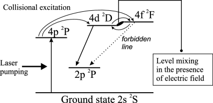
Figure 1: The scheme of laser-driven excitations of the Li i levels.

In the present experiments a lithium beam, produced by applying a Nd:YAG laser pulse onto a solid lithium target, is injected into the plasma region of interest. Another laser beam, which is used for the pumping, intersects the lithium beam at the point of interest to produce the LIF emission (see Fig. 2). The lithium beam density is so selected that it introduces a minimal disturbance in the region of diagnostics, while, on the other hand, is sufficient for yielding a satisfactory intensity of the desired transitions.

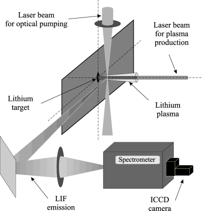
Figure 2: Application of LIF for the electric field measurements.

For the line-shape modeling, the method described in Ref. Evgeny was used. This method is capable of calculating line shapes under the simultaneous effects of the plasma micro- and macro-fields (both electric and magnetic ones). The forbidden transition from the $4f$ to the $2p$ level of Li i is caused mostly by the 4f–4d level mixing. The mixing of the 2p and 4f levels with other levels is negligible since the energy separations between these levels and 2p and 4f are significantly larger than the 4d–4f separation. Therefore, the 4f–4d energy separation is crucial for an accurate modeling. We have measured its value independently 4d-4f in order to resolve the ambiguity in light of the large spread in the values of this quantity in the available data sources.

III Experimental setup

In this experiment we employ a coaxial plasma configuration, shown in Fig. 3, in which plasma is initially injected to fill up the volume between the two coaxial electrodes. The cathode and anode diameters are 3.8 and 8.9 cm, respectively, and the plasma is injected over an axial length of 10 cm. A current pulse applied at one side of the coaxial line propagates through the plasma until the current channel reaches the vacuum section of the transmission line that is followed by a shorted end. This experimental configuration is commonly referred to as plasma opening switch (see e.g. POS ref and reference therein) and has been recently used for studying the interaction of the plasma with the propagating magnetic field PRL ; B-fieldRon ; Dynamics ; Rami .

The plasma prefill in the present experiment is produced by a flashboard plasma source and is injected inward through the transparent anode to fill up the A-K gap (see Fig. 3). The flashboard plasma with an electron density $n_{e}=2\times 10^{14}~{}\text{cm}^{-3}$ and electron temperature $T_{e}\simeq 5$ eV, almost uniform across the A-K gap, is mainly composed of protons and carbon ions (mainly C III-V). Since the heavier carbon ions flow at lower velocities than the protons, the carbon/proton relative abundance decreases towards the cathode.

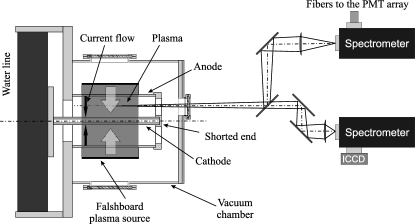
Figure 3: The layout of the coaxial transmission line and the diagnostic system.

The coaxial line is powered by an LC-water-line Marx generator. A current pulse of $160~{}\text{kA}$ with a rise time of $100~{}\text{ns}$ is then driven through the coaxial line. The upstream and downstream currents are measured by Rogowski coils placed at the output of the water-line and at the shorted end.

In the diagnostic technique here employed, the flashboard prefill plasma is doped with lithium using a laser-produced lithium beam (see Fig. 4). For the generation of the lithium beam, a Nd:YAG laser pulse (6 ns) is focused onto a surface of a metallic lithium target attached to one of the coaxial electrodes. The laser intensity was $5\times 10^{7}~{}\text{W/cm}^{2}$ on the target surface. The particle velocities in the laser-produced plasma plume were found to be $(1\div 10)\times 10^{5}~{}\text{cm/s}$. At the distance of $2.5~{}\text{mm}$ from the target, at which the electric field measurements are performed, the density of the lithium beam was $\simeq 7\times 10^{13}~{}\text{cm}^{-3}$ with an ionization degree of $\approx 65\%$, i.e., the electron density was $\simeq 4\times 10^{13}~{}\text{cm}^{-3}$. The electron temperature was $\simeq 0.5~{}\text{eV}$ (see Sec. IV.1). For the photopumping of the Li i 4p state, a tunable dye laser is used. This laser is pumped by an additional Nd:YAG laser pulse of 15 ns duration. In order to obtain the wavelength required for the photopumping ($\lambda_{2s-4p}=2741.2~{}\mathring{A}$), a wavelength extender for the generation of the second harmonic of the dye laser pulse is employed. Thus, the dye laser is tuned to generate a pulse at $\lambda_{dye}=5482.4$ Å (using a solution of Fluorescein 548 dye in methanol). The energy achieved at 2741.2 Å is $\simeq$1 mJ. The laser spectral width is 0.2 Å.

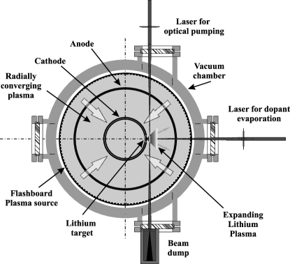
Figure 4: The cross section of the coaxial chamber, showing the dopant excitation scheme. Observations are performed in the direction perpendicular to the figure plane.

For measurements where recording of accurate spectral line profiles are important, experimental conditions for which the Doppler broadening is relatively small are preferable. The Doppler broadening that affects the line shapes in these measurements results from the lithium atom velocities in the axial (Z) direction (along the line of sight). In order to minimize this effect it is required to use a sufficiently long time delay between the laser pulse for target evaporation and the current pulse application. The reason is that the lithium atoms ejected from the target surface due to the laser pulse move away from the surface with velocities varying along the plasma column produced. Therefore, slow atoms reach the measurement region with longer delays. Generally, lower velocities in the propagation direction normal to the target surface are correlated with lower velocities in the transverse directions, which enabled us to achieve a satisfactorily low Doppler broadening in the axial direction. In the present experiment we used a time delay of 450 ns between the laser pulse employed for the target evaporation and the laser pulse employed for photopumping. Selecting longer time-delays decreases the amount of the atoms due to the lithium ionization processes that take place in the prefill plasma, thereby, reducing the signal-to-noise ratio. Therefore, the optimal delay was determined according to the requirement of minimal Doppler broadening but high enough signal intensity.

The diagnostic system consists of two 1-m UV-visible spectrometers equipped with 2400 grooves/mm gratings (see Fig. 3). The output of one spectrometer is collected by an optical-fiber array and transmitted to 10 photomultiplier tubes that allow the recording of the line-profile time-dependence (temporal resolution of 7 ns), while the output of the second spectrometer is recorded by a gated (down to 5 ns) intensified charge-coupled device (ICCD) camera, allowing for recording single gated broadband spectra. The spectral resolutions of both systems are $\simeq 0.2$ Å in the spectral range used. Since the induced fluorescence originates from the region along the pumping-laser path, observing the emitted radiation perpendicular to the pumping-beam direction allows for measurements with a high spatial resolution in 3 dimensions. In this case the spatial resolution along the line of sight is determined by the width of the pumping laser beam, which is $\simeq 1.5~{}\text{mm}$, whereas the resolution in the plane perpendicular to the line of sight is chosen by the spectrometer slit dimension (sub-mm scale). A detailed discussion of the spectral calibration and the determination of the instrumental response of the system can be found in Ref. 4d-4f .

IV Results

The measurements are performed in three stages. In the first stage we characterize the laser-produced lithium plasma used as a dopant. In principle, the dopant plasma could perturb the local conditions of the main prefill plasma, introducing uncertainties in the measurements. In order to minimize this perturbation, the dopant density must be kept lower than that of the main plasma. However, lowering the lithium density results in weakening the spectral lines of interest, thereby reducing the signal-to-noise ratio that is crucial for resolving the spectral profiles required for the determination of the electric field. To optimize the Li i dopant density, measurements of the lithium density, ionization degree, and expansion velocity were first performed with no plasma prefill.

In the second stage, with the optimal configuration of the lithium doping, the electric fields are measured in the plasma prefill (still without the application of the current pulse). These experiments yield the initial level of the electric field present in the plasma prior to the application of the current pulse. We refer to this field as a “background” electric field.

Finally, we measure the evolution of the electric fields generated during the conduction of the pulsed current.

IV.1 Diagnostics of the lithium dopant beam

Details of the measurements aimed at the diagnostics of the laser-produced lithium beam will be published separately f-lines . Here, we briefly describe the main results. Measurements were performed to determine the temporal evolution of the plasma parameters in the lithium beam at different distances from the target for various laser intensities in the range of $10^{7}$ - $10^{8}~{}\text{W/cm}^{2}$

A typical Li i spectrum in the wavelength range of interest (4603 Å), obtained at a distance of 2.5 mm from the target, is presented in Fig. 5. It is recorded by the ICCD camera with a time-gate of 10 ns correlated with the peak of the LIF signal. The figure shows the measured and simulated line shapes of the allowed 2p-4d and the nearby forbidden 2p-4f transitions. The line shape simulation, similar to that described in Ref. 4d-4f , show the individual contribution of each of the three broadening mechanisms: the Stark effect, Doppler, and instrumental.

The Doppler broadening can be estimated from the Li i velocities obtained from time-of-flight measurements. For the present measurements we used a time delay of 450 ns between the evaporating laser pulse and the photopumping laser pulse. At a distance of 2.5 mm from the electrode this delay corresponds to a velocity of $5.5\times 10^{5}~{}\text{cm/s}$. Since the Li i plume expands into a large solid angle, the transverse velocities are of the order of the longitudinal velocities. Indeed, a Doppler broadening of 2 eV, consistent with the velocities mentioned above, is obtained by deconvolving the known instrumental broadening function from the total line shape of the Li i 2p–3d transition (6104 Å) that is insensitive to the Stark effect under the present conditions.

Subsequently, the Stark-broadened spectrum for various values of the electron density $n_{e}$ is calculated, and convolved with the instrumental and the Doppler broadening functions. For these calculations, we used $T_{e}=0.5~{}\text{eV}$, adopted from the results of a collisional-radiative modeling of the temporal behavior of the Li i line intensities (described in Ref. thesis ).

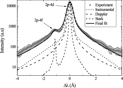
Figure 5: Measured and calculated Li i 2p–4d line shapes including the 2p–4f forbidden line.

From the line-shape calculations it is found that the measured spectrum cannot be satisfactorily fitted for any electron density. A good fit is rather obtained by assuming a combination of $n_{e}=(4\pm 0.7)\times 10^{13}~{}\text{cm}^{-3}$ and low frequency ($\lesssim\omega_{pi}$) oscillations with an amplitude of $\approx 3~{}\text{kV/cm}$ (see Fig. 5). Although assuming a higher electron density of $n_{e}\simeq 2\times 10^{14}~{}\text{cm}^{-3}$ (with no waves in the plasma) provides a satisfactory fit to the total intensity ratio of the allowed line to the forbidden line, the width of the 2p-4f line becomes significantly larger due to the wide spectrum of the microfield amplitudes under this assumption. This results in flattening of the forbidden peak, which is in disagreement with the observations.

IV.2 Effect of the plasma prefill injection on the Li i line shapes

We now describe the experiments in which the lithium beam is locally injected into the flashboard plasma that prefills the inter-electrode gap (still, without applying the main pulsed-current). The lithium target is attached to the cathode (the inner electrode, see Fig. 4). The plasma prefill parameters were obtained in a previous work from emission spectroscopy FB_ns . The plasma is found to have a nearly uniform electron density across the inter-electrode gap with $n_{e}\simeq 2\times 10^{14}~{}\text{cm}^{-3}$ and $T_{e}\simeq 5~{}\text{eV}$. Under these conditions the lithium atoms undergo substantial ionization and the density of neutral lithium arriving at the observation point is expected to be significantly lower than when the dopant is injected into vacuum, leading to reduced line intensities. Indeed, the intensity of the Li i 4603-Å line in the plasma prefill is found to be an order of magnitude lower than when the lithium beam is expanding in vacuum. Nevertheless, this intensity is still sufficient to provide a signal-to-noise ratio that is adequate for resolving the line profiles of interest. In these experiments the 2p-3d line is not useful for measuring the Doppler broadening since its upper level is no longer populated from the decay of the $n=4$ levels, as the latter are significantly depopulated through collisional ionization due to the higher prefill plasma density. Instead, here we use the 2s-2p line at 6708 Å that is also insensitive to the Stark effect. This line exhibits somewhat larger Doppler width than in the case of expansion into vacuum, corresponding to a temperature of $\simeq 2.5~{}\text{eV}$.

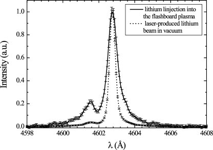
Figure 6: The spectrum of the 2p–4d and 2p–4f lines of Li i recorded in experiments with and without the presence of the flashboard prefill plasma. The spectra are normalized to have the same peak intensity for the 2p–4d lines.

In Fig. 6 we present a comparison of the profiles of the allowed 2p–4d and the forbidden 2p–4f lines emitted when the lithium beam is expanding in vacuum with those emitted with the flashboard plasma prefill. It is clearly seen that in the presence of the flashboard plasma the forbidden line has a substantially higher relative intensity and both lines are relatively broadened. Similarly to the previous case, also here we find that electric microfields, arising from the thermal electrons and ions, cannot explain the observations. The best fit is obtained by considering a combination of micro electric fields due to $n_{e}=(1\div 4)\times 10^{14}~{}\text{cm}^{-3}$ and the presence of a low frequency electric field of $8\pm 1~{}\text{kV/cm}$. We note that under these higher density conditions, the line profiles are less sensitive to the density, but the inferred density range agrees well with that found in a previous work FB_ns . The simulations also give an upper limit for the oscillation frequency of the additional electric field, $\approx 10~{}\text{GHz}$. This upper limit is of the order of $\omega_{pi}$ of the flashboard plasma, indicating that these oscillations can possibly be of the ion-acoustic type. Similar E-field intensities were measured in several positions, particularly in the positions where the E-field measurements were performed during the current application, as described in the next paragraph. We take this observed electric field of $8~{}\text{kV/cm}$ to be the upper limit of the collective fields present in the plasma prefill prior to the application of the high-current pulse; hereafter referred to as the “background” electric field.

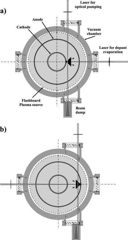
Figure 7: The two directions of the dopant injection. a) E-field measurement near the cathode. b) E-field measurement near the anode.

For performing measurements of electric fields also in the vicinity of the anode, the lithium target is attached to the anode and the evaporating laser beam is focused onto the target through a port in the vacuum chamber at the opposite side of the anode. The two different setups, allowing for measurements in the vicinity of the cathode and the anode, are schematically described in Fig. 7. Since the flashboard plasma source is located on an outside cylinder and its plasma flows radially inward, attaching the dopant-lithium target to the anode results in evaporated Li atoms flowing mostly in the same direction as the flashboard plasma flow, whereas when the Li target is attached to the cathode, the Li atoms flow opposite to the direction of the flashboard plasma flow. The line profiles obtained near the anode are compared to those obtained near the cathode. The comparison of the line profiles is performed for azimuthal and radial polarizations (the line of sight is along the axial direction). Interestingly, as shown in Fig. 8, the change of the dopant injection direction with respect to the flashboard plasma flow is found to affect the line profiles only in the azimuthal polarization. For the azimuthal polarization, the 2p–4f forbidden-line intensity is noticeably higher for the case where the dopant Li i atoms are injected opposite to the direction of the flow of the flashboard plasma (measurements near the cathode), while for the radial polarization the line profiles are found to be similar for the two cases of the dopant injection. The explanation for this effect is not clear yet. For the E-field measurements in the present study only the radial-polarization line-emission is used, for which no effect of the switching of the lithium injection direction on the line shapes is observed.

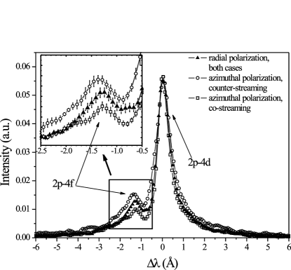
Figure 8: The profiles of the Li i 2p–4d and 2p–4f transitions measured for two orthogonal polarizations for the two directions of the dopant injection.

IV.3 Electric field measurements in the plasma under the high-current pulse

Knowledge of the effect of the prefill plasma on the dopant lithium line shapes and the corresponding electric fields allows for investigating the electric fields formed during the flow of the pulsed-current in the plasma. The measurements are performed at a distance of 2.5 mm from the electrodes (either the cathode or the anode) inside the inter-electrode gap at different axial positions. The field of view of the optical system covers a region between 2.2 and 2.8 mm from the electrodes. We note that estimates of the maximal sheath size give a much smaller distance from the electrodes, based on the known system inductance and the measured current. The electric field measured is thus in the plasma and not in the sheath. The arrangement of the measurement positions is shown in Fig. 9. The measurement positions are located symmetrically near the anode and near the cathode separated axially by 35 mm. The positions 1 and 4 in the plasma are located at a distance of $\approx 1.5$ cm from the generator-side plasma boundary. The boundary position is defined as the position beyond which (towards the generator) $n_{e}$ drops by more than a factor of 3 relative to that in the main part of the plasma. Due to the plasma expansion towards the cathode the plasma boundary is slightly farther from the measurement positions near the cathode than near the anode.

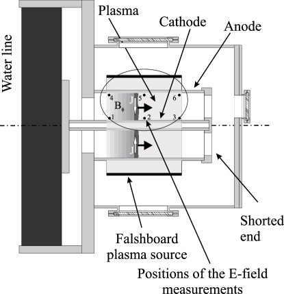
Figure 9: Positions for the E-field measurements during the current application. The positions are located symmetrically in the A-K gap having an axial separation of $35~{}\text{mm}$. The total length of the plasma is $\approx 10~{}\text{cm}$.

This setup allows for determining the velocity of the electric-field axial propagation at the two radial positions (near the anode and of the cathode). The temporal evolution of the electric field at each position is obtained by performing consecutive experiments, varying the time delay between the application of the current pulse and the application of the photo-pumping laser. The temporal resolution of the measurements (10 ns) is determined by the time-gate of the ICCD camera. In order to cover the entire duration in which the current flows through the plasma, the E-field is obtained at a minimum of 6 consecutive time intervals in each position. For overcoming the shot-to-shot irreproducibility, the results at each time are averaged over several discharges.

Figure 10: Comparison of the normalized spectral profiles prior and during the current pulse application. The measurements are performed at point 2. The delay between the current start and the beginning of the measurement is $40~{}\text{ns}$, corresponding to time of maximum E-field at point 2.

Figure 10 shows a comparison between the spectral profiles obtained at point 2 prior and after the current-pulse application. It is clearly seen that the lines broaden during the current conduction in the plasma, with the forbidden component rises in intensity relative to the allowed line and becomes shifted to shorter wavelengths. This demonstrates the rise of the E-field in the plasma during the current conduction. The recorded profiles are analyzed in the manner described in Sec. II, taking into account the effects of the plasma microfields, the Doppler broadening, and the instrumental broadening. This analysis yields the electric field amplitude as a function of time.

The inferred evolution of the E-fields at the 3 axial positions near the cathode and the anode are shown in Fig. 11. The error-bars in the figure reflect the statistical errors due to the shot-to-shot irreproducibility. In addition, a systematic error of up to 10% can be expected due to the finite accuracy of the line-shape modeling. For clarity, these have been omitted from the figure. Thus, the absolute value of the measured E-field has an additional error of 10%. The rise of the E-field in the vicinity of the cathode (Fig. 11a) is observed to be delayed between the different axial positions. This allows for determining the axial propagation velocity of the electric field, which is found to be $(1.5\pm 0.5)\times 10^{8}~{}\text{cm/s}$. The velocity is found to be approximately the same between points 1 – 2 and 2 – 3, therefore, the E-field propagation velocity is concluded to be constant over the entire pulse. Based on the 10-ns temporal resolution, the rise time of the E-field is inferred to be less than $10~{}\text{ns}$. The product of the field rise-time and the propagation velocity gives an estimate of the axial scale of the changes of the electric field. This scale of $1-2~{}\text{cm}$ could possibly be related to the width of the current channel, which in previous experiments was found to exhibit a similar scale, $\approx 1$ cm PRL .

In the vicinity of the anode one might expect somewhat lower E-field values. This is plausible due to the lower B-field near the anode and the higher fraction of heavy ions, since the latter leads to a higher electron density following the reflection of the protons by the propagating magnetic front. However, the E-field at point 4 was found to have an amplitude similar to the maximum obtained near the cathode, whereas at points 5 and 6 no rise in the field is observed within the measurement accuracy (see Fig. 11b). The E-field in point 4 rises at a delay compared to point 1, demonstrating a slower propagation of the E-field near the anode. Thus, when the current channel near the cathode reaches the vacuum section near the shorted end of the transmission line and as a result ceases to flow through the plasma, the current near the anode has still not reached point 5, and no E-field is generated at points 5 and 6. An upper limit for the field propagation velocity near the anode can thus be estimated by dividing the distance between point 4 and point 5 by the time interval between the field arrival at point 4 and the field arrival to the plasma-vacuum boundary (at the shorted-end side). This gives a velocity of $\simeq 7\times 10^{7}~{}\text{cm/s}$.

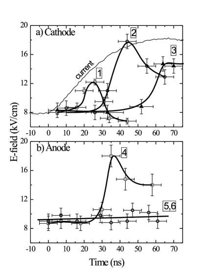
Figure 11: The evolution of the E-field obtained in the vicinity of the cathode and the anode (including the background field). The term $\textit{t}=0$ is the start of the current pulse.

We now estimate the net rise in the E-field due to the application of the current pulse, by subtracting from the measured total E-field ($E_{tot}$) the background field $E_{bg}$, found in the plasma prefill prior to the current application (see Sec. IV.2). A simple subtraction of this background from the measured E-field is not always correct. In order to demonstrate this fact, let us assume that some external quasi-static field $E_{ex}$ at a certain direction (e.g., the Hall field) is formed in the plasma in addition to the already present randomly directed, fluctuating background field. On a spatial scale smaller than the typical scale of the fluctuations, where the background field has a distinguished orientation, the background and the external fields should be summed up as vectors. Then, the sum of the fields must be averaged over all possible directions of the background field, since in the measurements the field of view of the optical system is assumed to be larger than the fluctuation scale. As a result, the mean value of the total measured field is given by $\displaystyle\bar{E}_{tot}=\sqrt{E_{ex}^{2}+E_{bg}^{2}}$.

Table 1 summarizes the results of the E-field measurements. The first column presents the position of the measurement. The other columns give the total measured E-field and the field obtained after the subtraction of the background field of $8.0\pm 1.0~{}\text{kV/cm}$ near the cathode and $9.0\pm 1.0~{}\text{kV/cm}$ near the anode. The Table also gives the inferred axial propagation velocity of the field ($V_{E}$).

Table 1: Summary of the peak E-field parameters.

Position	Peak E-field (kV/cm)		$V_{E}~{}(\text{cm/s})$
	Total	Without $E_{bg}$
Cathode
z = 1 cm (pos. 1)	$12.0\pm 0.5$	$9.0\pm 1.1$
z = 4.5 cm (pos. 2)	$17.8\pm 1.0$	$16.0\pm 1.4$	$1.5\pm 0.5\times 10^{8}$
z = 8 cm (pos. 3)	$14.5\pm 1.0$	$12.1\pm 1.4$
Anode
z = 1 cm (pos. 4)	$18.0\pm 1.8$	$15.5\pm 2.0$	$<7.0\times 10^{7}$
z = 4.5 cm (pos. 5)	$9.0\pm 1.0$	0
z = 8 cm (pos. 6)	$9.0\pm 1.0$	0

V Discussion

In the following, we demonstrate that the time-resolved measurements of the electric field in several locations in the plasma lead to two main results. The first is that the electric fields observed are probably the Hall electric fields resulting from the current flow in the plasma, and the other result is that turbulent electric fields observed in the plasma prefill prior to the current application may provide the anomalous collisionality required for the previously observed broadening of the current channel.

V.1 E-field generation due to the Hall effect

Magnetic field measurements, based on Zeeman spectroscopy, performed in a separate study Weingarten_Beams98 , using the same experimental setup, show that the B-field propagates faster near the cathode than near the anode, giving rise to a 2D-structure of the B-field propagation. We attribute this behavior to the decrease of the magnetic field intensity with increasing radius (the anode is the outer electrode) and to the increasing fraction of the heavy ions (carbon ions) in the plasma prefill closer to the anode. The parameters of the magnetic field and plasma prefill are listed in Table 2. It is expected that the rise in the E-field amplitude at each point coincides with the arrival of the current channel, namely, the arrival of the magnetic field front at that point. Indeed, the measured velocities of the magnetic field penetration, $1.2\pm 0.2\times 10^{8}~{}\text{cm/s}$ near the cathode and $5\pm 2\times 10^{7}$ cm/s near the anode Weingarten_Beams98 , are consistent with the velocities of the E- field propagation found here, $(1.5\pm 0.5)\times 10^{8}~{}\text{cm/s}$ near the cathode and approximately a factor of two slower near the anode.

Table 2: The parameters of the plasma and the magnetic field in the present experiment. The terms $n_{C}$ and $n_{p}$ are, respectively, the densities of the carbon and proton components of the plasma, and $Z_{\text{eff}}^{\text{C}}$ is the effective charge of the carbon ions.

Parameter	Cathode	Anode
$r$ $\text{(}{cm})$	1.9	4.45
$B_{\text{peak}}$ (T)	$1.2\pm 0.2$	$0.5\pm 0.1$
$n_{e}$ $\text{(}{cm}^{-3})$	$(2\pm 0.5)\times 10^{14}$	$(2\pm 0.5)\times 10^{14}$
$n_{p}/n_{C}$	$\approx 9$	$\approx 1$
$Z_{\text{eff}}^{\text{C}}$	$\approx 3$	$\approx 3$

In a quasi-neutral plasma the electric field is given by Ohm’s law:

$$\vec{E}=\frac{\vec{j}\times\vec{B}}{cn_{e}e}-\frac{1}{c}\vec{v}_{i}\times\vec{B}+\frac{1}{\sigma}\;\vec{j},$$ (1)

where $B$ is the magnetic field, $j$ is the current density, $v_{i}$ is the ion velocity, $\sigma$ is the plasma conductivity, and $c$ is the speed of light in vacuum. Here, the electron inertia and pressure are neglected. We now show that the measured electric field in the vicinity of the cathode is close to the electric field calculated by this expression when only the first (Hall) term on the right-hand-side is considered. The second term, which results from ion pushing Huba is shown to be smaller than the Hall term. The contribution of the third term is discussed in Sec. V.2. For evaluating the Hall term and comparing it to the present electric field measurements we use previous measurements of the magnetic field and density PRL ; Weingarten_Beams98 .

Although the B-field measurements are highly informative, they do not allow for the reconstruction of the spatial distribution of the B-field due to the small number of the measurement positions in the A-K gap. Nevertheless, these measurements demonstrate a strong correlation between the rise of the magnetic field at each measurement position and a drop of the electron density (see, e.g., PRL ). We note that the prominent density drop is closely related to the phenomenon of ion-species separation PRL , mentioned in Sec. I, in which the magnetic field only penetrates into the heavier component of the plasma (carbon ions) while the light ions (protons) are reflected ahead by the magnetic field front. In Ref. Weingarten_Beams98 a map of the electron density distribution was measured at different instants of the current conduction in an experimental setup similar to the present one. These data show that the density drop propagates axially, exhibiting different propagation velocities at different radial positions. Thus, assuming the density drop in the A-K gap is correlated with the arrival of the magnetic field front everywhere, the measured evolution of the density map can be used to determine the distribution of the B-field front.

We now fit an analytical expression for the magnetic field temporal distribution. Based on the previous measurements PRL ; B-fieldRon we approximate the B-field axial distribution at each radial position by a step-like function of a front width $\delta$, i.e., the B-field rises within a distance $\delta$ that corresponds to the current-channel width. This step front propagates axially with a constant velocity. The propagation velocity is lower at larger radii, similarly to the density drop Weingarten_Beams98 . At the plasma boundary, $z=0$, the magnetic-field temporal behavior was found to be similar to that of the generator current, approximated by $I_{up}=I_{max}\sin\left(\frac{\pi t}{2\tau}\right)$, where $\tau$ is the time corresponding to the peak-current. Therefore, we assume that the amplitude of the field in the back of the step-front (which is the height of the step) also rises in time as $sin\left(\frac{\pi t}{2\tau}\right)$. For the radial distribution of the magnetic field we assume that the field at the rear of the field-front decreases towards the anode as $1/r$, due to the cylindrical geometry of the experiment. Under these assumptions we find that the magnetic field can be approximated by:

$$\displaystyle B(r,z,t)=B_{0}\frac{r_{c}}{r}\sin\left(\frac{\pi t}{2\tau}\right)\times$$

$$\displaystyle\times\frac{1}{2}\left[1-\tanh\left(2\,\frac{\displaystyle z-v_{c}\frac{r_{c}}{r}t}{\delta}\right)\right],$$ (2)

where $B_{0}$ is the peak magnetic field, $r_{c}$ and $r_{a}$ are the cathode and anode radii, $0<t<\theta$ (here we focus on the period of the current flow through the plasma lasting until $\theta=70~{}\text{ns}$ that denotes the arrival of the current channel at the plasma transmission-line boundary), $v_{c}$ is the B-field propagation velocity near the cathode, and $\delta$ is the current-channel width. In our experiment $\tau\approx\theta$. The variables $r$ and $z$ are limited by $r_{c}<r<r_{a}$ and $0<z<z_{end}$, where $z_{end}$ is the position of the plasma transmission-line boundary. In the calculations, the current channel width $\delta$, which is assumed to be broadened by diffusion, varies in time as $\delta=\lambda_{e}+\delta_{\theta}t/\theta$, where $\lambda_{e}$ is the electron skin depth. The term $\lambda_{e}+\delta_{\theta}$ is the front-width at the instant $t=\theta$. Since at time $t=\theta$ $\delta$ is measured to be about $1~{}\text{cm}$, which is much larger than $\lambda_{e}$, we obtain $\delta_{\theta}\approx\delta(t=\theta)\approx 1~{}\text{cm}$. The comparison of the map of the B-front propagation determined from the previous measurements of the electron density drop to the map generated using the semi-analytical formula (2) is shown in Fig. 12, demonstrating a good agreement between the two approaches.

Figure 12: The map of the magnetic field propagation a) obtained from the electron density evolution (contours denote the location at which the density starts to drop), b) generated using Eq. (V.1) (here the contours are the locations where the magnetic field is 0.2 T). The numbers on the plot represent the time in nanoseconds relative to the beginning of the current pulse. The solid circles in (b) represent the positions of the present E-field measurements.

Using the analytic form of the magnetic field and the fact that $\vec{B}=B\vec{e}_{\varphi}$, the Hall electric field is expressed by:

$$\displaystyle\vec{E}_{Hall}=\frac{[rot\vec{B}\times\vec{B}]}{4\pi\>n_{e}\>e}=$$ (3)

$$\displaystyle=\frac{1}{4\pi\>n_{e}\>e}\left[\vec{e}_{r}\left(B\>\frac{1}{r}\frac{\partial(rB)}{\partial r}\right)+\vec{e}_{z}\left(B\frac{\partial B}{\partial z}\right)\right]$$ .

Finally, by inserting Eq. (V.1) into Eq. (3), the axial ($E_{Hall,z}$) and radial ($E_{Hall,r}$) components of the electric field are found to be:

$$\displaystyle E_{Hall,z}=\frac{B_{0}^{2}\>r_{c}^{2}\>\sin^{2}\left(\frac{\displaystyle\pi t}{2\tau}\right)}{8\pi\>n_{e}\>e\>r^{2}\>\delta}\>\left[1-\tanh(\zeta)\right]\times$$

$$\times\left[1-\tanh^{2}(\zeta)\right],$$

$$\displaystyle E_{Hall,r}=\frac{B_{0}^{2}\>r_{c}^{3}\>v_{c}\>t\>\sin^{2}\left(\frac{\displaystyle\pi t}{2\tau}\right)}{8\pi\>n_{e}\>e\>r^{4}\>\delta}\>\left[1-\tanh(\zeta)\right]\times$$

$$\times\left[1-\tanh^{2}(\zeta)\right],$$ (5)

where $\displaystyle\zeta=2\,\frac{\displaystyle z-v_{c}\frac{r_{c}}{r}t}{\delta}$.

We now compare the magnitude of the measured E-field with the calculated $E_{Hall}$ using the expressions (V.1) and (5). We note that for this comparison, knowledge of the electron density is essential. Here, again, we use the previous measurements by Weingarten et al. Weingarten_Beams98 . We assume that the magnetic field reflecting the protonic component of the plasma and thereby causing the density to drop, penetrates only into the carbon plasma PRL . The electron density of the carbon plasma (penetrated by the magnetic field) is determined here for each position at the time of the arrival of the magnetic front at the transmission-line boundary of the plasma. At this time, at the generator side of the plasma, namely at point 1, the electron density drops from $2\times 10^{14}~{}\text{cm}^{-3}$ to $5\times 10^{13}~{}\text{cm}^{-3}$. In the middle of the plasma (at point 2) the density only drops to $10^{14}~{}\text{cm}^{-3}$, and at the transmission-line boundary of the plasma (at point 3) no density drop is found, rather a slight rise to $\approx 2.5\times 10^{14}~{}\text{cm}^{-3}$ is observed. Using these data, the evolution of $n_{e}$ is incorporated into the calculations of $E_{Hall}$ by synchronizing the change of the local value of the electron density with the rise of the local magnetic field, namely $\displaystyle n_{e}\left(z,r,t\right)=n_{0}-\Delta n\left(z,r\right)\frac{B\left(z,r,t\right)}{B_{max}\left(r,t\right)}$. Here, $\Delta n\left(z,r\right)$ denotes the density drop at the particular position for which the electric field evolution is calculated, and $\displaystyle B_{max}=B_{0}\frac{r_{c}}{r}\sin\left(\frac{\pi t}{2\tau}\right)$.

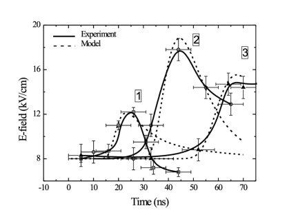
Figure 13: Comparison of the electric field evolution observed in the experiments with the Hall-electric field calculated using the semi-analytical approximation. The calculated total Hall-field is a vector sum of $E_{Hall,z}$ and $E_{Hall,r}$. The background E-field of 8 kV/cm, found in the flash-board plasma, is added to the calculated values in the manner described in Sec. IV.2.

Thus, the evolution of the Hall electric field is calculated for the three different axial positions at which the electric field measurements were performed. Figure 13 gives a comparison between the calculation results and the experimental data near the cathode. The Hall field presented is the magnitude of the electric field including its axial and radial components, to which the $8~{}\text{kV/cm}$ turbulent background has been added according to $E=\sqrt{E^{2}_{r}+E^{2}_{z}+E^{2}_{bg}}$ (see Sec. IV.2). It is seen that the calculated Hall-field fits well the measured values, except for point 1 at relatively late times. The relatively large deviation seen for point 1 can possibly be explained by the more pronounced $n_{e}$ drop observed at this point, which may reduce the turbulent background E-field, contrary to our assumption in the model that the background field is constant.

Such a good agreement between the experimentally measured electric field and the calculated Hall electric field, based on the B-field and density measurements, as shown in Fig. 13, suggests that the observed E-field is most likely the Hall field, generated by the current. Although a thorough understanding of the field evolution requires a self-consistent modeling that, for example, would also consider the ion reflection and species separation observed in the experiment, this agreement indicates that the Hall field could play a crucial role in the magnetic field penetration.

The model discussed here predicts the E-field near the anode (point 4) to be a factor of 4 lower than that near the cathode at point 1 (B-field drops by a factor of 2 near the anode, see Table 2), in disagreement with the measurements (see Fig. 11). A possible explanation is a rise of the turbulence near the anode during the current flow. In order to test this explanation, one could measure the axial velocities of the accelerated ions both near the anode and near the cathode. Since the ions accelerate axially mostly due to the Hall-field, if indeed the electric field is mostly turbulent near the anode then the axial ion velocities near the anode will be substantially lower than they are near the cathode, but the velocity distribution will be much broader.

The contribution of the ion motion to the electric field in Ohm’s law (the second term of the RHS of Eq. (1)) is small. This contribution can be estimated by comparing $\left|\vec{j}/en\right|$ to $\left|\vec{v_{i}}\right|$. Approximating the magnitude of the current density by $\left|\vec{j}\right|\simeq cB/4\pi\delta$, using the measured ion velocities from Ref. PRL , and assuming the ions are accelerated in the direction perpendicular to the B-field front, we find the contribution of the convective term in Eq. (1) to be much smaller than the contribution of the Hall term. If instead of using the measured ion velocities we use the MHD velocity $\left|\vec{v_{i}}\right|\simeq B/\sqrt{4\pi\rho}$ (where $\rho$ is the mass density ahead of the current front) as the maximal ion velocity, we find that the contribution of the Hall term is larger than that of the ion motion as long as $\delta<\left(c/en\right)\sqrt{\rho/4\pi}$ (the effective ion skin depth). Here, $\rho\cong 6.7\times 10^{-10}~{}\text{g/cm}^{3}$ yields an effective ion skin depth of $\cong 2.3~{}\text{cm}$ that is much larger than $\delta\cong 0.5~{}\text{cm}$ (the current-channel width observed in the experiments), thus the ion term is expected to be smaller.

V.2 Anomalous collisionality

As suggested in Sec. IV.2, the background electric field may be attributed to an ion-acoustic instability in the plasma. In this case, this electric field should cause a relatively strong electron collisionality in the plasma prior to the application of the current. Here we describe the effect of such a strong collisionality on the magnetic-field evolution and the current distribution.

Following Ref. Weingarten_turbulence , the effective collision frequency $\nu^{tur}_{ei}$ associated with the ion-acoustic turbulent electric fields in the plasma is:

$$\nu^{tur}_{ei}\simeq\omega_{pe}\frac{\langle E^{2}\rangle}{8\pi n_{e}kT_{e}}.$$

Assuming that the turbulent E-field is of the order of the background E-field of $8~{}\text{kV/cm}$ measured prior to the current application, and using $n_{e}=5\times 10^{13}~{}\text{cm}^{-3}$ and $T_{e}=10~{}\text{eV}$ ($10~{}\text{eV}$ being the upper limit of the electron temperature in the plasma prefill), the expected collision frequency is $\nu^{tur}_{ei}\simeq 10^{10}~{}\text{Hz}$. This frequency is much higher than Spitzer’s collision frequency, which for the above parameters is $2\times 10^{8}~{}\text{Hz}$. Such a high collision frequency is expected to increase the rate of magnetic field penetration into the plasma and also to broaden the current channel.

In spite of the relatively high anomalous collision frequency suggested here, it is still insufficient to explain the fast B-field penetration by diffusion that requires collision frequency of about $7\times 10^{11}~{}\text{Hz}$  B-fieldRon . In addition, step-like spatial profile of the magnetic field is inconsistent with the exponential decay predicted by diffusion. A different mechanism, such as the Hall-field induced mechanism Gordeev ; Fruchtman , is thus expected to cause the fast magnetic field penetration. Still, the high anomalous collision frequency may help to explain the observed broad current-channel, not understood thus far. According to Ref. Weingarten_turbulence , in a steady Hall-induced penetration the current-channel width is estimated to be:

$$\delta\simeq L~{}\frac{\nu_{ei}}{\omega_{pe}}\frac{c}{V_{Ae}},$$

where $V_{Ae}$ is the Alfvén velocity of electrons, $\displaystyle V_{Ae}\equiv B/(4\pi n_{e}m_{e})^{1/2}$ ($m_{e}$ is the electron mass), and $L$ is the inter-electrode spacing. Although in the present experiment the plasma and field dynamics do not reach a steady state, we use this relation to obtain an estimate for the current-channel width, assuming Hall-induced penetration. For $L=2.5~{}\text{cm}$ and the anomalous collision frequency estimated above, we find that $\delta\simeq 5~{}\text{mm}$. This value is an order of magnitude larger than the electron skin-depth $c/\omega_{pe}\sim 0.5~{}\text{mm}$ and consistent with the measurements  Weingarten_Beams98 used for our model ($\delta(t=\tau)=1~{}\text{cm}$). Thus, while the anomalous collision frequency estimated from the turbulent electric fields is insufficient to explain the rate of magnetic field penetration, it does explain reasonably well the current channel width. We note that in a previous investigation Weingarten_turbulence it was concluded otherwise, based on an estimated upper level of a $5~{}\text{kV/cm}$ electric field. However, in that experiment the plasma source was a plasma gun rather than a surface flashover as in the present work. Also, the previous E-field measurements might have been related to a secondary plasma, since they were based on hydrogen line-emission that also originated at electrode sputtering Arad_flashboard .

The anomalous collision frequency predicted above is about three times higher than the minimal collision frequency required for a collisional current channel dominated by the Hall-field penetration FruchtmanPRA , $\nu_{min}=B/\left[L(8\pi m_{e}n_{e})^{1/2}\right]$, which is estimated to be $3\times 10^{9}~{}\text{Hz}.$ This further supports the possibility of a Hall-field induced magnetic-field penetration.

We note that for $B<0.3~{}\text{T}$ the value of $\nu^{tur}_{ei}$ is larger than the electron gyrofrequency, meaning there is no electron magnetization and the resistive term (the third term on the RHS of Eq. (1)) is thus dominant in determining the electric field at the beginning of the current conduction. Therefore, the Hall mechanism is not applicable in these conditions. The collisionality, though rather high, also cannot explain the velocity of the magnetic field penetration at this early stage of the pulse and the question regarding the mechanism of the initial magnetic field penetration remains open.

VI Summary

For the first time the electric fields in current-carrying plasmas are measured with high spatial and temporal resolutions. This is achieved by a diagnostic method that is based on line-shape analysis of dipole-forbidden transitions combined with laser spectroscopy. The measured electric fields exhibit a good agreement with the Hall field calculated using measurements of the time-dependent magnetic-field and density distributions in the current-carrying plasma. These results indicate that in the present experiment the Hall mechanism can be dominant in the magnetic field penetration into the plasma. Moreover, it is noteworthy that the modeled Hall field, which depends linearly on $1/n_{e}$, reproduces well the present E-field measurements, particularly in light of the sharp density drop observed due to the ion-species separation phenomenon. It is important to note, however, that in order to further conclude that the Hall electric field induces the magnetic field penetration, as suggested in Refs. Gordeev ; Fruchtman ; FruchtmanPRA , it is yet to be shown that the evolution of the electric fields must be consistent with the magnetic field propagation in accordance with Faraday’s law:

$$\frac{\partial\mathbf{B}}{\partial t}=-\frac{1}{c}\mathbf{\nabla\times E}\;$$ (6)

A rather high level of the electric field ($\approx 8$ kV/cm) is observed in the plasma prefill prior to the pulsed current application. Such electric fields, if present in the entire prefill plasma, may give rise to an anomalous collisionality that is consistent with the Hall mechanism and may help explaining the observed current channel width. A clarification of this effect and the nature of this possible turbulence can be a subject of future investigations.

- (1) B.V. Weber, R.J. Commisso, R.A. Meger, J.M. Neri, W.F. Oliphant and P.F. Ottinger, Appl. Phys. Lett. 45, 1043 (1984)
- (2) R. Shpitalnik, A. Weingarten, K. Gomberoff, Ya. Krasik, and Y. Maron, Phys. Plasmas 5, 792 (1998).
- (3) A. Weingarten, R. Arad, Y. Maron, A. Fruchtman, Phys. Rev. Lett. 87, 115004 (2001).
- (4) R. Arad, K. Tsigutkin, Y. Maron, A. Fruchtman, and J.D. Huba, Physics of Plasmas 10, 112-125 (2003).
- (5) R. Arad, K. Tsigutkin, A. Fruchtman and Y. Maron, Phys. Plasmas 11 (9), 4515 (2004).
- (6) S. Kingsep, Yu. V. Mochov, and K. V. Chukbar, Sov. J. Plasma Phys. 10, 495 (1984); A. S. Kingsep, K. V. Chukbar, and V. V. Yankov, in Reviews on Plasma Physics, edited by B. Kadomtsev (Consultants Review, New York, 1990), Vol. 16, p. 243.
- (7) V. Gordeev, A. V. Grechikha, Ya. L. Kalda, Sov. J. Plasma Phys. 16, 95 (1990); A. V. Gordeev, A. V. Grechikha, A. V. Gulin, and O. M. Drozdova, ibid. 17, 381 (1991).
- (8) A. Fruchtman, Phys. Fluids B 3, 1908 (1991).
- (9) A. Fruchtman, Phys. Rev. A 45, 3938 (1992).
- (10) A. Weingarten, S. Alexiou, Y. Maron, M. Sarfaty, Ya. E. Krasik, and A. S. Kingsep, Phys. Rev. E 59, 1096 (1999).
- (11) M. Baranger and B. Mozer, Phys. Rev. 123 (1), 25 (1961).
- (12) H.-J. Kunze and H. R. Griem, Phys. Rev. Lett. 21, 1048 (1968).
- (13) U. Rebhan, N. Wiegart, and H.-J. Kunze, Phys. Lett. 85A (4), p. 228 (1981).
- (14) J. Hildebrandt and H.-J. Kunze, Phys. Rev. Lett. 45, p. 183 (1980).
- (15) U. Rebhan, J. Phys. B: At. Mol. Phys. 19, pp. 3847-3857 (1986).
- (16) C. Burrell and H.-J. Kunze, Phys. Rev. Lett. 29, p. 1445 (1972).
- (17) K. Kawasaki, K. Takiyama, and U. Oda, Jap. Journ. Appl. Phys. 27 (1), pp. 83-88 (1988).
- (18) B. Knyazev, S. Lebedev, and P. Melnikov, Sov. Phys. Tech. Phys. 36 (3) pp. 250-256 (1991).
- (19) Yu.V. Ralchenko and Y. Maron, J. Quant. Spectr. Rad. Transf. 71, 609 (2001).
- (20) E. Stambulchik, Y. Maron, J. Quant. Spectr. Rad. Transf. 99 (1-3), 730 (2006).
- (21) K. Tsigutkin, E. Stambulchik, Y. Maron, and A. Tauschwitz, Physica Scripta 71, 502 (2005).
- (22) Special issue on fast opening vacuum switches, IEEE Trans. Plasma Sci. PS-15, 1987.
- (23) R. Doron, R. Arad, K. Tsigutkin et al., Phys. Plasmas 11, 2411 (2004).
- (24) K. Tsigutkin, E. Stambulchik, V. Bernshtam, and Y. Maron, “Forbidden-line spectroscopy of electric fields in plasmas”, to be published.
- (25) K. Tsigutkin, “Investigation of electric fields in plasmas under pulsed currents”, PhD thesis, Weizmann Institute of Science 2005.
- (26) A. Weingarten, V. Bernshtam, A. Fruchtman, C. Grabowski, Y. Krasik, and Y. Maron, IEEE Transaction on Plasma Science, 27, 1596 (1999).
- (27) A. Weingarten, C. Grabowski, A. Fruchtman, and Y. Maron, Proc. of 12th Int. Conf. on High-Power Particle Beams (BEAMS’98), Vol.1, p.346
- (28) J.D. Huba, J. M. Grossmann, and P. F. Ottinger, Phys. Plasmas 1, 3444 (1994).
- (29) R. Arad, K. Tsigutkin, Yu.V. Ralchenko, and Y. Maron Phys. Plasmas 7, 3797 (2000)
- (30) A. V. Gordeev, A. S. Kingsep, and L. I. Rudakov, Physics Reports vol. 243, 215 (1994).