Polymers in a vacuum

Abstract

In a variety of situations, isolated polymer molecules are found in a vacuum and here we examine their properties. Angular momentum conservation is shown to significantly alter the average size of a chain and its conservation is only broken slowly by thermal radiation. The time autocorrelation for monomer position oscillates with a characteristic time proportional to chain length. The oscillations and damping are analyzed in detail. Short range repulsive interactions suppress oscillations and speed up relaxation but stretched chains still show damped oscillatory time correlations.

The properties of polymer chains have been investigated extensively over the past fifty years degennes but the vast majority of these studies have been concerned with situations where they are in a solution or a melt. However there are some situations where polymer molecules are essentially in a vacuum. Desorption and ionization of polymers, often by lasers is carried out during mass spectrometry, in order to characterize desorbed proteins. This has many important applications including the understanding of cancer CaldwellCaprioli . Polymer molecules of many different kinds have been detected in interstellar media NewCarbonChains and although they have predominantly had less than 10 units, the detection of new species is an active area of research. It might also be possible to employ optical tweezers on biomolecules such as DNA and manipulate them in a vacuum, in a manner similar to what is now done routinely in aqueous solution block .

To aid in the possible experimental observation of such systems, some basic properties of isolated polymers in a vacuum are considered here. The first question that we ask is how their statistics are modified from those in solution. Solvents will compete with intra-chain attractions so that above the $\theta$ temperature degennes , a polymer chain will be swollen. Without the solvent present, this would imply that a chain at the same temperature would be collapsed. But at high enough temperatures, entropy will dominate over energy, and a polymer, just like a liquid, will then want to expand into a gas, or self avoiding phases. Because carbon-carbon bonds are very strong, it might then be possible to find some species where a polymer will become swollen in isolation for long enough periods of time to be observable. Even if it turns out that this is not possible, polymers through desorption often carry a charge, and this additional coulomb repulsion is quite substantial, at $500K$ it is $\approx 33k_{B}T$ for two electrons $1~{}nm$ apart. This will serve to stretch a chain. Such a situation is a possibility in the desorption and ionization of proteins done in mass spectrometry experimentsCaldwellCaprioli .

It might then appear that the statistics of this system are identical to that of a chain in a solvent, with some modification of interaction parameters. However one important difference is the conservation of angular momentum that we might expect to see in this case as opposed to a polymer in a solvent. In statistical mechanics, this conservation law is ordinarily ignored and is not expected to make a difference to system properties when the number degrees of freedom are large. However we will see that for a polymer in isolation it has a significant effect on its size, even when the total angular momentum is zero. The effects of angular momentum conservation have been recently studied in self-gravitating systems laliena where it leads to different phases for some models for finite angular momentum.

The starting point for this situation is the formula for the classical entropy in the microcanonical ensemble with conservation of linear and angular momentum of a system with total potential energy $U$ laliena . However we can safely transform this into the canonical ensemble at temperature $T$ using the usual argument that the fluctuations in the energy at constant temperature are small for a large number of degrees of freedom. However we are still keeping the $\delta$ function constraint on the total angular momentum $\bf L$. Using the Fourier representation for a $\delta$ function and integrating over the momenta, the partition function becomes

$$Z(T,{\bf L})\propto\int e^{i{{\bf k}}\cdot{\bf L}}e^{-\frac{T}{2}({\bf k}\cdot{\bf I}\cdot{\bf k})-\beta U}\prod_{i=1}^{N}d^{3}{\bf r}_{i}d^{3}{\bf k}$$ (1)

where $N$ is the number of monomers, $\bf I$ the moment of inertia tensor of a polymer conformation, and the center of mass is fixed to zero. Adding a term $\epsilon\sum_{i}r_{i}^{2}$ to $\beta U$ allows one to differentiate $\ln Z$ with respect to $\epsilon$ to obtain the r.m.s. size of a chain defined as $\langle R^{2}\rangle\equiv\frac{1}{N}\langle\sum_{i=1}^{N}r^{2}_{i}\rangle$

For an “ideal” or “phantom” chain footnote:ideal with ring topology, the calculation can be done exactly DeutschToBePublished giving the results shown in Fig. 1. The rescaled angular momentum $L^{\prime}\equiv L\sqrt{12}/(N\sqrt{Tml})$ where $m$ is the mass and $l$ is the step length, which both can be taken equal to $1$.

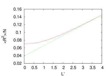
Figure 1: (Color Online) The variation of the size of a chain versus its angular momentum for a ideal ring chain. The straight line is the asymptotic slope which can be obtained through a simple analysis.

At $L=0$, $\langle R^{2}\rangle/N=.07$. Results using a simulation method described below give $.071$ which are the same to within the error bars. This is substantially below, $1/12\approx.083$, the value of the same quantity where conservation of angular momentum is not enforced. When averaged over all angular momenta, the size of the chain must agree with the non-conserved case, and because high $L$ chains will have greatly extended conformations, this must be compensated for by correspondingly compact configurations for small $L$.

To obtain the asymptotic behavior for large $L$, using a much simpler argument, we expect that in this limit the dominant configuration of the chain will be a highly stretched circle of radius $R$ rotating symmetrically about the axis of angular momentum. We minimize the free energy, of a polymer taking into account both its kinetic energy and elastic energy yielding $R^{2}/N=L^{\prime}/(12\pi)$ again choosing $l=m=1$. The straight line in fig. 1 has the same slope.

The case of self avoiding (swollen) chains ($R\sim N^{\nu}$ with $\nu\approx 3/5$), is qualitatively similar. and the asymptotic scaling can be easily worked out along similar lines as above, giving $R\propto L^{4/11}N^{1/11}$.

The total angular momentum however, is not conserved. Interaction with thermal photons will cause the angular momentum to equilibrate on a time scale that we will now estimate. First we consider the flux of electromagnetic energy emitted by a single polymer. The emission of thermal radiation per unit area of a black body is given by the Stephan-Boltzmann law $S=\sigma T^{4}$, where $\sigma$ is the Stephan-Boltzmann constant. However this greatly overestimates the radiation because of the weak efficiency of small objects in emitting light of a far greater wavelength. Calculations for metal nanoparticles (which should be better emitters than dielectrics) give a suppression factor of less than $10^{-3}$ when the nanoparticles are $50A$ in radius radiation_small . This gives a ratio of $k_{B}T$ to emitted power of $6\times 10^{-6}s$. The relaxation time as we will see below scales roughly as $N^{2}$. The microscopic hopping time typical for such a system is $10^{-12}s$, meaning that the relaxation time for $N=100$ is roughly $10^{-8}s$. Thus thermal photon equilibration is more than two orders of magnitude slower than the time-scale for relaxation of a chain. Therefore one expects to see transitions in the time averaged radius of gyration of a chain as photons are emitted and absorbed by the polymer. This might be observable in the signature of noise seen in light scattering.

We now turn to a study of the dynamics of these polymers and we will see that in this respect the situation is very different from that of a polymer in a solvent. In a solvent, models for dynamics for the most part consider monomers connected together by linear springs, thermal noise, solvent drag, and hydrodynamic interactions. However in a vacuum, the last three terms are not present, which leaves us with Newtonian dynamics for linear springs, but this will never thermalize, so nonlinear forces must be considered.

One might first guess that sufficient nonlinearity would introduce strong enough dissipation of individual modes so that the behavior would be similar to that of the Rouse model Rouse , which describes a “free draining” chain. That is one where individual monomers experience a drag proportional to their velocity. However this violates Galilean invariance, as we shall discuss in more detail below. Moreover one dimensional systems are notorious for not being able to equilibrate energy well, and there are many well studied instances where this problem is known to occur. Perhaps the best known example of this is the Fermi Pasta Ulam chain FPU . For small enough energies this system shows strong recurrences in amplitude of modes above which it equilibrates BermanIzrailev Models that are even more nonlinear such as the Sinai-Chernov “Pen Case model” pencase do not suffer from this problem, however they still exhibit highly non-local time correlations, with universal power law decays DeutschNarayan , which is a general result for one dimensional chains that are momentum and energy conserving NarayanRamaswamy

So we first consider the dynamics of a chain neglecting any self avoiding interactions, but using an athermal highly nonlinear model for the reasons mentioned above. Thus we have chosen a model where monomers of equal mass are coupled together by links of fixed length. Aside from this constraint, there is no potential energy. The monomers can freely rotate but there is no coupling to an outside system so that there is no dissipation or random noise term. The model rigorously satisfies conservation of energy, momentum and angular momentum. An efficient method for evolving such chains was developed so that despite the large number of length constraints, the computation for each time step scales linearly with the number of monomers. The details will be published elsewhere DeutschToBePublished . The angular momentum, center of mass and energy were monitored to ensure that their drifts due to numerical error remained small for all data used.

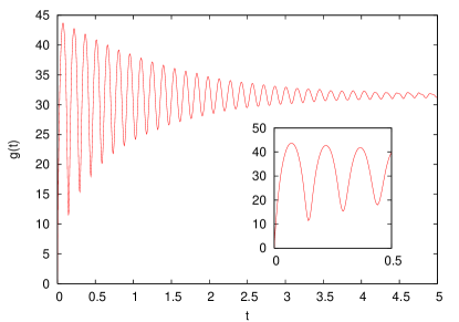
Figure 2: (Color Online) The autocorrelation function $g(t)$ as defined in Eq. (2) for a chain of 128 monomers. The inset shows the beginning of the plot at a higher magnification, where the initial linear increase and cusps are apparent.

The monomer-monomer autocorrelation function defined as

$$g(t)=\langle\frac{1}{N}\sum_{i=1}^{N}|{\bf r}_{i}(t)-{\bf r}_{i}(0)|^{2}\rangle$$ (2)

was calculated for chains of different lengths and is displayed in Fig. 2 for $N=128$ averaged over $24,000$ runs. This is very unlike the correlation function for a polymer in solution which shows a smooth slow increase, not the wildly oscillatory form seen here. The period of these oscillations scales as chain length. This is what one would expect for a linear model with no friction, because the lowest mode of oscillation has spring constant $\propto 1/N$, and the mass is $\propto N$ giving a period $\propto N$. At first sight, it is surprising that the oscillations are so weakly damped in a model that is so highly nonlinear. To understand this better, we analyze this problem in terms of linear modes. The relaxation time of the chain is then given by the damping time for these oscillations. In terms of a Fourier decomposition along the arclength of the chain, we can model the correlation function as $\langle r_{k}(0)r_{k}^{*}(t)\rangle=\langle|r_{k}|^{2}\rangle Re(\exp((i\omega_{k}-\lambda_{k})t)$ and because $|r_{k}|^{2}\propto 1/k^{2}$,

$$g(t)\propto\sum_{k}\frac{(1-\cos(\omega_{k}t))}{k^{2}}e^{-\lambda_{k}t}$$ (3)

and this can be used to fit the numerical data. In this expression the $\omega_{k}$’s represent the frequencies of oscillation. We therefore expect that for small $k$ that $\lambda_{k}$ will be small in comparison to $\omega_{k}$, the only other relevant frequency scale for each term in the summation.

For small $t$, and no dissipation ($\lambda_{k}=0$), the small $t$ behavior of $g(t)$ in the above expression can easily be shown to be $\propto t$. Yet for short times this shows that the mean square displacement follows the same law as a diffusive process. For longer times, oscillatory behavior will be seen but will be asymmetric, showing cusps at the minima and parabolic maximum. These same qualitative features persist for small $\lambda_{k}$ and are also in quite good agreement with the simulation data shown in Fig. 2.

It is clear from the data that $\omega_{k}\propto k$, just as one would expect from a linear system of springs. The damping appears to fit best to a form close to $\lambda_{k}\propto k^{2}$. Fitting this to different chain lengths, $N=64$ and $128$, gives a relaxation time $T_{rel}\propto N^{(1.85\pm.15)}$. Note that in the case of one dimensional heat conduction, it has been found that even with highly nonlinear models DeutschNarayan , asymptotic large $N$ behavior is difficult to study as more than $10^{4}$ particles must be considered to get a good estimate of critical exponents. Therefore it is possible that the exponent found is off by $\sim 10\%$ of its asymptotic value.

This value of the relaxation time scales closely to what is seen in the Rouse model although in that case the physics is very different as there is no inertia term and no rapidly oscillatory behavior. In the case we consider here, the origin of this time is due to nonlinear coupling of different modes resulting in the slow translation to decoherence as time progresses.

As mentioned above, this problem is quite similar to that of a one dimensional nonlinear chain of particles. In that case the system is also characterized by long wavelength oscillations that slowly decohere. But there, the relaxation time $T_{rel}\propto N^{3/2}$ which is different than the polymer case. If the polymer chain was stretched by a constant force so that it was quasi-one dimensional, one would expect the same $N^{3/2}$ scaling for the relaxation time.

To understand the damped oscillatory behavior of the correlation function, in Eq. 3, we consider what kind of coarse grained linear stochastic equation would best approximate the evolution of ${\bf r}(s,t)$, the position of the chain at arclength $s$ and time $t$. Because the system has Galilean invariance, there can be no $\dot{\bf r}$ term for the damping, as center of mass velocity is conserved. By symmetry, the lowest order damping term must be $C\partial^{3}{\bf r}/\partial t\partial^{2}s$ where C is a constant. Adding in inertia, random forcing $\bf\xi(s,t)$ and chain connectivity gives

$$\frac{\partial^{2}{\bf r}}{\partial t^{2}}=\Big{(}1+C\frac{\partial}{\partial t}\Big{)}\frac{\partial^{2}{\bf r}}{\partial s^{2}}+{\bf\xi(s,t)}$$ (4)

In relation to the above analysis, this gives a damping $\lambda_{k}\propto k^{2}$ for small k. Such a model matches fairly well the numerical data footnote:RelaxTime .

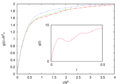
Figure 3: (Color Online) The scaled autocorrelation function $g(t)/\langle R^{2}\rangle$ versus $t/N^{p}$, for three chain lengths, $N=32$, $64$, and $128$ with short-range repulsive interactions. The inset shows $g(t)$ for an $N=32$ chain with equal charges at both ends that cause it to stretch.

Such a proposal for internal damping for polymer chains in connection with Cerf friction degennes ; Cerf has been made before MacInnes using a nonrigorous derivation that gives rise to the same third order derivative term as in eqn. 4. Adding such a term to the Rouse equation provides an explanation of experiments CerfExp on extensional relaxation of polymers in solvent. Solvents with different viscosities were considered to extrapolate to the limit of zero viscosity, and the results can be interpreted using such a term.

As one might expect, the inclusion of repulsive interactions between monomers suppresses the oscillations that are seen in the ideal chain. For the sake of efficiency, soft-core potentials were added between between monomers having a potential of the form $\beta V(r)=2(1-(r/l)^{2})^{5}$. Statistics of such chains with total angular momentum of zero were measured and the size scaling exponent gave $\nu=.596\pm.01$ in good agreement with the well known three dimensional value.

In Fig. 3 the autocorrelation function for these chains, see Eq. 2, is plotted for chain lengths $N=32$, $64$, and $128$, on scaled axes so that they coincide for short times. The vertical axis is $g(t)/\langle R^{2}\rangle$ and the horizontal one is $t/N^{p}$, with $p$ chosen to fit short times best. With $p=1.15$, the plots coincide well over half of the vertical range, from $0$ to $1$. However the long time behavior for $N=32$ is noticeably above the longer length chains. However $N=64$ is only slightly above $N=128$, and given the correlated error bars, this is barely statistically significant. This is strong evidence that for large $N$ the correlation function approaches the scaling form $g(t)=N^{2\nu}f(t/N^{p})$, and therefore the relaxation time for this chain is $\propto N^{p}$, with $p=1.15\pm.05$. Note that this is much smaller than that of the ideal chain discussed above, presumably because long range interactions along the chain backbone allow much faster equilibration of energy and momentum footnote:LongerRelaxTime . We expect the time it takes a chain segment to move of order its average size $R_{g}$ should be $R_{g}$ divided by the center of mass speed for of order half the chain, $\sim N^{-1/2}$, which gives $t_{rel}\sim N^{1.1}$.

Finally we contrast this with what happens if charges are added to both ends. With charged protein molecules observed in mass spectrometry, a similar situation could also occur. The inset in Fig. 3 shows the autocorrelation function for this case, where the end to end distance is $10.03$, about one third of the chain’s arclength. The parameters were chosen so that there is still a substantial amount of interaction between neighboring monomers, but the chain is still quite stretched. Here one can clearly see oscillations in $g(t)$, intermediate in behavior between the ideal chain and interacting cases.

In conclusion, the equilibrium statistics and dynamics of polymers in a vacuum have many interesting properties. The addition of angular momentum conservation significantly alters chain statistics. The subtle power-law time correlations found in momentum conserving one dimensional systems can lead to dynamics that are oscillatory and show unusual scaling properties. It is hoped that this work will provide impetus for further experimental observation of these fascinating systems.

The author thanks Larry Sorensen for very useful discussions.

References

- (1) P.G. de Gennes “Scaling Concepts in Polymer Physics” Cornell University Press (1985).
- (2) R.L. Caldwell, and R.M. Caprioli, Mol. Cell. Proteomics 4, 394–401 (2005)
- (3) P. Thadeus, M.C. McCarthy, M.J. Travers, C.A. Gottlieb, and W. Chen, Faraday Discuss., 109, 121 (1998).
- (4) M.D. Wang, H. Yin, R. Landick, J. Gelles, and S.M. Block, Biophysical Journal 72 1335 (1997).
- (5) V Laliena, Phys. Rev. E 59, 4786 (1999).
- (6) One with only nearest neighbor connectivity and no other interactions between monomers.
- (7) J.M. Deutsch, to be published.
- (8) Y.V. Martynenko, L.I. Ognev, arXiv:physics/0503025 (2005).
- (9) P. E. Rouse, J. Chem. Phys. 21, 1272 (1953).
- (10) E. Fermi, J. Pasta, and S. Ulam, Studies of nonlinear problems (Los Alamos Document LA-1940, 1955).
- (11) For a review see G.P. Berman and F.M. Izrailev, Chaos 15, 015104 (2005) and references therein.
- (12) Ya. G. Sinai and N.I. Chernov, Russian Math. Surveys (3) 42, 181 (1977).
- (13) J.M. Deutsch and O. Narayan, Phys. Rev. E 68, 010201 (2003). J.M. Deutsch and O. Narayan, Phys. Rev. E 68, 041203 (2003).
- (14) O. Narayan and S. Ramaswamy, Phys. Rev. Lett. 89, 200601 (2002).
- (15) The fact that the terminal relaxation time found scales as and not , means that will have a very weak dependence on which if actually correct would imply that there is some nonlocality in the equation of motion. However it is likely that this deviation is due to the finite length of the chains considered, as experience in the one-dimensional heat conduction problem has shown.
- (16) R. Cerf, C.R.Acad. Sci. Paris. 286B, 265 (1978)
- (17) D.A. MacInnes, J. Poly. Sci. 15 465 (1977); D.A. MacInnes, J. Poly. Sci. 15 657 (1977).
- (18) R. Cerf C.R.Acad. Sci. Paris. 230, 81 (1950), J. Leray, Ph.D. Thesis Strasbourg, 1959.
- (19) One can still not rule out the possibility of a longer relaxation time with a signature too small to be measurable.