General Depolarized Pure States: Identification and Properties

Abstract

The Schmidt decomposition is an important tool in the study of quantum systems especially for the quantification of the entanglement of pure states. However, the Schmidt decomposition is only unique for bipartite pure states, and some multipartite pure states. Here a generalized Schmidt decomposition is given for states which are equivalent to depolarized pure states. Experimental methods for the identification of this class of mixed states are provided and some examples are discussed which show the utility of this description. A particularly interesting example provides, for the first time, an interpretation of the number of negative eigenvalues of the density matrix.

1 Introduction

Describing and quantifying entangled quantum states and preventing errors during quantum dynamical processes are important and, at this time, unsolved problems. Each of these has important implications for the development of reliable quantum information processing devices. In order to tackle these problems, it is common to broaden our knowledge and understanding by developing key examples. This is our approach here as we examine a particular class of quantum states.

This work was motivated by a desire to be able to identify and distinguish a certain class of mixed quantum states, and their properties, experimentally. This will rely, in part, on the existence of the Schmidt decomposition [2] which provides a canonical form for bipartite pure states. The Schmidt decomposition is used to identify and quantify entanglement in bipartite quantum systems [3]. Such systems are primitives for a host of quantum communication and computation protocols. However, such protocols are invariably subject to noise which diminishes their advantage over classical protocols. Noise, for most quantum systems, is difficult to identify and protect against, although there are several promising methods (see for e.g. [4] and references therein). Here we introduce a generalized Schmidt decomposition for a class of mixed quantum states which we hope will aide both with the problem of understanding entanglement and our ability to correct for noisy quantum processes. Our decomposition does not retain all of the useful properties which make the pure-state version so important. However, it does allow us to devise some useful tools for measuring properties of an important class of states.

The Schmidt decomposition is described by a set of real coefficients that is invariant under local unitary operations. All entanglement measures on pure states, such as the von Neumann entropy of a reduced density operator, can be computed from this set. However, this decomposition is known only to exist for general bipartite pure states (see for example [5]) and some multipartite pure states [6, 7]. Therefore, quantifying entanglement in terms of this decomposition does not work in general. For mixed states, several entanglement measures exist, most of which are difficult to calculate, though some interesting special cases for bipartite systems can be solved. For example, for two qubits one can calculate the Entanglement of Formation (EoF) [8] which is the amount of entanglement required to form a particular state. It is also known how to calculate the EoF for Werner states [9], isotropic states [10] and rotationally invariant states [11]. However, at this time there is no canonical Schmidt decomposition for mixed states and no efficient method by which to analytically compute the entanglement of general mixed states.

One might anticipate that a generalization of the Schmidt decomposition would aid in the description of entangled states. One such generalization is given by the Schmidt number [12], which is equal to the maximum Schmidt rank (or number of Schmidt coefficients) in a pure state decomposition of a mixed state, minimized over all decompositions. This quantity constitutes the minimum Schmidt rank of the pure states needed to construct a state, and is an entanglement monotone [12]. Here we consider another special case which is a Schmidt decomposition for depolarized pure states (DPS) which are those states obtained by mixing the identity operator on the state space with a single pure state. These have many interesting properties and have been studied in the literature since these states are fairly easy to manipulate. For example, one may compute properties such as channel capacities [13, 14], entanglement (specific instances) [15, 16], and more recently, it has been shown that noisy operations may be turned into depolarizing operations [17]. The set of DPS which we define here includes, not only pure states which have undergone a depolarizing operation, but also states which, if initially decoupled from their environment, cannot be obtained in this way. All states in our DPS class can be brought into a similar canonical form using local unitary operations.

The DPS are important to understand in part because they have a fairly simple form. This form has $2D-1$ real parameters as opposed to $D^{2}-1$ parameters for a generic mixed state in a $D$ dimensional Hilbert space. They are also important to understand because any map can be brought to the depolarizing form by a simple sequence of quantum operations. Therefore a complicated quantum computing process in the presence of noise can be brought into this form which produces states with relatively few relevant parameters. This allows a direct comparison of inequivalent noise processes by projecting them into the same class.

In this article we discuss methods for experimentally determining whether this form has indeed been produced. We find expressions for the fidelity and the trace distance for this class of mixed states, and are also able to show that the negativity is more easily quantified for bipartite DPS. More importantly perhaps, we provide a bound for the number of negative eigenvalues for bipartite DPS and show that the number of negative eigenvalues can indicate the type of entanglement present in the system, e.g. qubit-qubit vs. qutrit-qutrit. These results support a limited form of a conjecture by Han, et al. [18] about the maximum number of negative eigenvalues for a bipartite state. We emphasize that our results provide an experimentally detectable qualitative and quantitative measure of entanglement.

The paper is organized as follows. In Section 2.1 we review the coherence vector parameterization of the density operator. In Section 2.2 we provide a geometric interpretation of DPS in terms of the coherence vector parameterization. Section 2.3 demonstrates that there exists a type of Schmidt decomposition for depolarized pure states when there exists a Schmidt decomposition for the corresponding pure state. In Section 3 we provide two ways in which to identify these states experimentally, and describe physical maps which give rise to DPS beginning in an unknown pure state. In Section 4 we discuss the insight that we gain into bipartite entanglement given our construction. We then conclude with a summary and some open questions in Section 5. Some examples of the formalism are given in Appendix A.

2 Schmidt form for DPS

In this section we provide several forms for the DPS which will be used for various calculations in later sections.

2.1 The coherence, or Bloch, vector

The generalized coherence vector, or Bloch vector representation [19, 20, 21, 22] will provide a convenient geometric picture for several parts of our argument. For a two-state system the description is well-known. The general case for an $D$-dimensional system is presented here and the two-state system will be seen to be a special case.

Any density operator $\rho$ belonging to the set of bounded linear operators $\mathcal{B}(\rho)$ with Hilbert space dimension ${\rm dim}(\mathcal{H})=D$, can be expanded in a basis consisting of the identity operator and an operator basis for $\mathfrak{su}(D)$, the algebra of $SU(D)$. Throughout this work, we represent the latter with a set of Hermitian, traceless matrices, $\{\lambda_{i}\}_{i=1}^{D^{2}-1}$ which obey the following orthogonality condition

$$\mbox{Tr}(\lambda_{i}\lambda_{j})=2\delta_{ij}.$$ (1)

The commutation and anticommutation relations for this set are summarized by the following product formula

$$\lambda_{i}\lambda_{j}=\frac{2}{D}\delta_{ij}{\bf 1}_{D}+ic_{ijk}\lambda_{k}+d_{ijk}\lambda_{k}.$$ (2)

Here, ${\bf 1}_{D}$ is the $D\times D$ unit matrix, the $c_{ijk}$ are the structure constants of the Lie algebra represented by these matrices, and the $d_{ijk}$ are referred to as the components of the totally symmetric “$d$-tensor.”

The density matrix for an $D$-state system can now be written in the following form

$$\rho=\frac{1}{D}\left({\bf 1}_{D}+\sqrt{\frac{D(D-1)}{2}}\;\vec{n}\cdot\vec{\lambda}\right),$$ (3)

where $\vec{n}\cdot\vec{\lambda}=\sum_{1}^{D^{2}-1}n_{i}\lambda_{i}$. For $D>2$ the following conditions characterize the set of all pure states,

$$\vec{n}\cdot\vec{n}=1,\;\;\;\mbox{and}\;\;\;\vec{n}\star\vec{n}=\vec{n},$$ (4)

where the “star” product is defined by

$$(\vec{a}\star\vec{b})_{k}=\sqrt{\frac{D(D-1)}{2}}\;\frac{1}{D-2}d_{ijk}a_{i}b_{j}.$$ (5)

For $D=2$, the condition $\vec{n}\cdot\vec{n}=1$ alone is sufficient [23]. Note that

$$n_{i}=\sqrt{\frac{D}{2(D-1)}}\;\;\mbox{Tr}\left(\rho\lambda_{i}\right).$$ (6)

To recover the case of the two-state Bloch sphere, note that the constants $1/D$ and $\sqrt{D(D-1)/2}$ reduce to $1/2$ and $1$ respectively, and the $d_{ijk}$ are identically zero, so the second condition in Eq.(4) is not required. In fact, as noted, it cannot be satisfied.

2.2 Depolarized Pure States

Throughout this paper we focus on a special class of mixed states, the depolarized pure states (DPS). Such states are given by a (not necessarily convex) sum of the identity operator and a pure state:

$$\rho_{d}\equiv(1-p)\frac{1}{D}{\bf 1}_{D}+p\rho^{\prime},$$ (7)

for $\rho^{\prime}$ some pure state. By the unit trace and positivity conditions, we have $-1/(D-1)\leq p\leq 1$. Letting $c_{D}=\sqrt{D(D-1)/2}$, we may rewrite this in a more suggestive form as

$$\rho_{d}=\frac{1}{D}\left({\bf 1}_{D}+c_{D}\;p\vec{n}\cdot\vec{\lambda}\right).$$ (8)

We note that for $D>2$ the characterization is unique, i.e. $\rho_{d}$ corresponds to a depolarized form of a single pure state with coherence vector $\vec{n}$. This is because the condition $\vec{n}\star\vec{n}=\vec{n}$ demands that both $\vec{n}$ and $-\vec{n}$ cannot correspond to physical pure states. Hence, any vector of the form $p\vec{n}$ has a unique purification, namely $\vec{n}$. For $D=2$ this is not the case because both $\vec{n}$ and $-\vec{n}$ correspond to pure states. From this latter form, we may interpret the DPS as arising from the affine map: $\vec{n}\mapsto p\vec{n}$, on the $D^{2}-1$ dimensional real vector space of coherence vectors.

This provides a geometric description of the set of depolarized pure states. The space of DPS with a given $p$ is isomorphic to the set of pure states (for $D>2$). (See for example [24] and references therein.) To see the geometry more explicitly, note that the DPS can be written in the form

$$\rho_{d}=\frac{1}{D}\left({\bf 1}_{D}-pW\left[\begin{array}[]{ccccc}1&&&&\\ &1&&&\\ &&\ddots&&\\ &&&1&\\ &&&&-(D-1)\end{array}\right]W^{\dagger}\right).$$

Note that the same matrix $W$ will diagonalize both the pure state and the depolarized pure state.

We will make use of this form to analytically compute the trace distance and fidelity between two DPS. The fidelity between two density matrices is defined by

$$F(\rho,\sigma)=\mbox{Tr}\Big{[}\sqrt{\sqrt{\rho}\sigma\sqrt{\rho}}\Big{]}^{2}.$$ (9)

We consider two DPS both in a $D$ dimensional Hilbert space,

$$\begin{array}[]{lll}\rho_{d}&=&(1-p)\frac{{\bf 1}}{D}+p\left|\Psi\right\rangle\left\langle\Psi\right|\\ \sigma_{d}&=&(1-q)\frac{{\bf 1}}{D}+q\left|\Phi\right\rangle\left\langle\Phi\right|\\ \end{array}$$

where $-\frac{1}{D-1}\leq p\leq 1$ and the overlap in their purifications is $F(\left|\Psi\right\rangle,\left|\Phi\right\rangle)=|\langle\Psi\left|\Phi\right\rangle|^{2}=f$. The (square root) of the fidelity is

$$\begin{array}[]{lll}\sqrt{F(\rho_{d},\sigma_{d})}&=&(D-2)\sqrt{a}+\sum_{\pm}\Bigg{[}\frac{2a+(b+2c)f+d+b(1-f)}{2}\pm\\ &&\sqrt{\frac{((b+2c)f+d-b(1-f))^{2}}{4}+(b+c)^{2}(1-f)f}\Bigg{]}^{\frac{1}{2}},\\ \end{array}$$ (10)

where the parameters are given by:

$$\begin{array}[]{lll}a&=&\frac{(1-p)(1-q)}{D^{2}},\\ b&=&\frac{(1-p)q}{D},\\ c&=&\frac{q}{D}\big{(}\sqrt{((D-1)p+1)(1-p)}-(1-p)\big{)},\\ d&=&\frac{(1-q+Dqf)}{D^{2}}\big{(}(D-2)p+2-2\sqrt{((D-1)p+1)(1-p)}\big{)}\\ &&+\frac{2(1-q)}{D^{2}}\big{(}\sqrt{((D-1)p+1)(1-p)}-(1-p)\big{)}.\end{array}$$

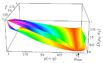
Figure 1: Distance measures between two depolarized pure states (DPS) in a $D=9$ dimensional Hilbert space with equal polarizations $p=q$. The Bures metric, trace distance, and fidelity satisfy the following inequalities [25]: $B(\rho,\sigma)^{2}/2\leq D(\rho,\sigma)\leq\sqrt{1-F(\rho,\sigma)}$ and surface plots of these three functions are shown. The value $p_{\rm min}=-1/80$ is the minimum polarization of depolarized pure states which are obtainable from a completely positive map. (We call these physically depolarized pure states, cf. Sec. 3.4.)

The square root of the fidelity can be converted into a metric, specifically the Bures metric via $B(\rho,\sigma)=\sqrt{2-2\sqrt{F(\rho,\sigma)}}$, and an angle $A(\rho,\sigma)=\cos^{-1}\sqrt{F(\rho,\sigma)}$. In the pure state case, the Bures metric is the Euclidean distance between the two pure states with respect to the norm on the state space and the cosine of the angle between the states is the overlap. The Bures metric between two mixed states can be interpreted as the Euclidean distance between purifications of the mixed states minimized over all such purifications.

One can also compute the distance (in the trace norm) between two mixed states. The distance is

$$D(\rho,\sigma)=\frac{1}{2}\mbox{Tr}|\rho-\sigma|_{\rm tr},$$ (11)

where the trace norm is defined $|O|_{\rm tr}=\sqrt{O^{\dagger}O}$. For the two DPS,

$$\begin{array}[]{lll}D(\rho_{d},\sigma_{d})&=&\frac{1}{2}\Bigg{[}\frac{(D-2)|q-p|}{D}+\sum_{\pm}\Big{|}\frac{(q-p)(1-D/2)}{D}\\ &&\pm\sqrt{(\frac{p+q-2qf}{2})^{2}+q^{2}(1-f)f}\Big{|}\Bigg{]}\\ \end{array}$$ (12)

The distance between two mixed states with the same coherence vector magnitude $p=q$ is simply $D(\rho_{d},\sigma_{d})=(1-f)|p|$. The distance and fidelities of equally polarized pure states are plotted in Fig. 1. Notice that beginning in a pure state, i.e. $p=1$, the distance and Bures metric between states with $f<1$ will decrease under a depolarizing map until both states are mapped to the identity. For even stronger maps, i.e. $p<0$ the distance begins to increase again. As discussed in Sec. 3.4, the minimum value of polarization obtainable by a physical map acting on input pure states is $p_{\rm min}=-1/(D^{2}-1)$. At this value, the distance between the output states is $D(\rho_{d},\sigma_{d})=\frac{1-f}{D^{2}-1}$. Thus we find that the distance (fidelity) between initially pure states is not a monotonically decreasing (increasing) function of the depolarization strength.

2.3 Schmidt Decomposition For A Pure Bipartite State

To fix notation, let us recall the Schmidt decomposition for a pure state of a bipartite quantum system in $D=D_{A}\times D_{B}$ dimensions with subsystems $A$ and $B$ which have dimension $D_{A}$ and $D_{B}$ respectively. Without loss of generality, we will assume that $D_{A}\leq D_{B}$. Now, let

$$\rho_{AB}^{\prime}=\left|\Psi^{\prime}\right\rangle\!\!\left\langle\Psi^{\prime}\right|,$$ (13)

where

$$\left|\Psi^{\prime}\right\rangle=\sum_{i,\mu}a_{i\mu}\left|{\phi_{i}}^{\prime}\right\rangle_{A}\left|{\psi_{\mu}}^{\prime}\right\rangle_{B}.$$ (14)

According to the Schmidt decomposition [2], there exist unitary matrices $U$ which acts only on the first subsystem, and $V$ which acts only on the second subsystem, such that $\left|\Psi\right\rangle$ can be written in the form:

$$\left|\Psi\right\rangle=\sum_{j}b_{j}\left|\phi_{j}\right\rangle_{A}\left|\psi_{j}\right\rangle_{B},$$ (15)

where the set $\{\left|\phi\right\rangle_{A}\}$ ( $\{\left|\psi\right\rangle_{B}\}$) forms an orthonormal basis for $A$ ($B$). In other words, there are local unitary transformations, $U$ and $V$ such that

$$U\otimes V\left|\Psi^{\prime}\right\rangle=\sum_{j}b_{j}\left|\phi_{j}\right\rangle_{A}\left|\psi_{j}\right\rangle_{B},$$ (16)

where

$$b_{j}\delta_{j\nu}=\sum_{i,\mu}U_{ij}a_{i\mu}V_{\mu\nu}.$$ (17)

and $U,V$ can chosen so that the $\{b_{j}\}$ are real and positive. We will say that $a_{i\mu}$ is “diagonalized” [26] by the local unitary transformations $U$ and $V$. The reduced density matrices $\rho_{A}=\mbox{Tr}_{B}(\rho)=\sum_{j}b_{j}^{2}\left|\phi_{j}\right\rangle_{A}\left\langle\phi_{j}\right|$ and $\rho_{B}=\mbox{Tr}_{A}(\rho)=\sum_{j}b_{j}^{2}\left|\psi_{j}\right\rangle_{B}\left\langle\psi_{j}\right|$ have the same eigenvalues $b_{j}^{2}$.

Now, let us consider the density operator

$$\rho^{\prime}=\frac{{\bf 1}_{AB}}{D}+\left(\sum_{ik,\mu\beta}a_{i\mu}a_{k\beta}^{*}\left|\phi_{i}^{\prime}\right\rangle_{A}\left\langle\phi_{k}^{\prime}\right|\otimes\left|\psi_{\mu}^{\prime}\right\rangle_{B}\left\langle\psi_{\beta}^{\prime}\right|-\frac{{\bf 1}_{AB}}{D}\right).$$ (18)

Defining the matrix $\sqrt{|p|}\;a_{i\mu}\equiv c_{i\mu}$, we see that if the matrix $a_{i\mu}$ can be diagonalized by $U$ and $V$, then $\sqrt{|p|}\;a_{i\mu}$ can be diagonalized by the same $U$ and $V$.

$$\rho_{d}=\frac{{\bf 1}_{AB}}{D}(1-p)+p\sum_{j,j^{\prime}}b_{j}b_{j^{\prime}}\left|\phi_{j}\right\rangle\!\!\left\langle\phi_{j^{\prime}}\right|\otimes\left|\psi_{j}\right\rangle\!\!\left\langle\psi_{j^{\prime}}\right|.$$ (19)

Therefore, there exists a preferred local unitary basis for depolarized pure states and we refer to this preferred basis as the Schmidt decomposition for DPS.

Furthermore, we can provide a relationship between the eigenvalues of the reduced density matrices for the two subsystems. Tracing over the subsystem $B$ produces

$$\rho_{d_{A}}=\mbox{Tr}_{B}(\rho_{d})=\frac{{\bf 1}_{A}}{D_{A}}(1-p)+p\sum_{j}b_{j}^{2}\left|\phi_{j}\right\rangle\!\!\left\langle\phi_{j}\right|.$$ (20)

Now, let us suppose that there are $n$ non-zero eigenvalues of $\rho^{\prime}_{A}=\mbox{Tr}_{B}(\rho^{\prime})$ given by $\{b_{j}^{2}\}$ with $\sum_{i=1}^{n}b_{i}^{2}=1$. (Alternatively, we could let the sum go to $D_{A}$ noting that for some $i$, the eigenvalue could be zero.) Then the eigenvalues of $\rho^{\prime}_{A}$ are $\{\frac{1}{D_{A}}(1-p)+pb_{i}^{2}\}_{i=0}^{n-1}\sqcup\{(1-p)/D_{A}\}^{D_{A}-n}$. Tracing over the subsystem $A$ produces

$$\rho_{d_{B}}=\mbox{Tr}_{A}(\rho_{d})=\frac{{\bf 1}_{B}}{D_{B}}(1-p)+p\sum_{j}b_{j}^{2}\left|\psi_{j}\right\rangle\!\!\left\langle\psi_{j}\right|.$$ (21)

The eigenvalues of $\rho^{\prime}_{B}$ are given by $\{\frac{1}{D_{B}}(1-p)+pb_{i}^{2}\}_{i=0}^{n-1}\sqcup\{(1-p)/D_{B}\}^{D_{B}-n}$.

There are two properties of the Schmidt decomposition which make it particularly useful and are properties which one would want to preserve in any generalization. It specifies (i) preferred bases of (ii) bi-orthogonal states. It is clear that property (i) is retained for DPS. This relies on the fact that it is unique for pure states [5] barring a degeneracy in the spectrum of one of the subsystems.

The Schmidt decomposition for general bipartite DPS is the preferred basis which agrees with the pure state Schmidt decomposition counterpart of the DPS. This definition clearly retains the property (i) and it can be generalized to any system with a corresponding pure state Schmidt decomposition. For example those described by a multipartite Schmidt decomposition [6, 27] will also have corresponding set of DPS.

Can this preferred basis be used to quantify the entanglement of the system? Certainly this is not true for the entropy of the partial trace as can be seen by considering the extreme case where $p=0$. However, we will discuss how the Schmidt form helps identify and distinguish certain types of entangled states in Section 4.

3 Preparation and Identification of DPS

It is now pertinent to ask, how does one know if a density matrix describes a system whose state is in the class DPS? Is there a way to characterize maps which give rise to these states? This section will provide the answers to these questions.

3.1 State Tomography

Using state tomography the elements of the density matrix may be determined. There are several ways in which to do this, some of which are more efficient than others. For our purposes, it is assumed that state tomography data has been collected and from it the coherence vector $\vec{n}$ determined, for example via Eq. (6).

From Eq.(4) the coherence vector of a pure state satisfies $\vec{n}\star\vec{n}=\vec{n}$. For a DPS, $\vec{n}\rightarrow p\vec{n}$, so that $\vec{n}\star\vec{n}\rightarrow p^{2}\vec{n}\star\vec{n}$, etc. From these relations, it is clear that all invariants described in [21] can be calculated by noting that for a DPS $[\vec{n}\star]^{r}\vec{n}\cdot\vec{n}=p^{r+2}$. Therefore the invariants reduce to the simplified form which is obtained by replacing $\vec{n}$ with $p$ everywhere and neglecting the types of products. In other words,

$$\begin{array}[]{lll}\vec{n}\cdot\vec{n}&=&p^{2},\\ \vec{n}\star\vec{n}\cdot\vec{n}&=&p^{3},\\ \vec{n}\star\vec{n}\star\vec{n}\cdot\vec{n}&=&p^{4},\mbox{ and so on.}\end{array}$$

These conditions may be stated equivalently, and more succinctly, as

$$\vec{n}\cdot\vec{n}=p^{2},\;\;\;\mbox{and}\;\;\;\vec{n}\star\vec{n}=p\vec{n}.$$ (22)

Note that, similar to the pure state conditions, these two conditions alone determine the set of eigenvalues for the density operator.

Note also that the DPS with $p<0$ and with $p>0$ can be distinguished with the unitary invariant $\vec{n}\star\vec{n}\cdot\vec{n}$ (provided $D>2$). Hence given some prior certificate that the state is a DPS, we obtain complete spectral information from the measurement of $\vec{n}\cdot\vec{n}$ and $\vec{n}\star\vec{n}\cdot\vec{n}$ including the value of $p$.

Alternatively, one may examine the eigenvalues of the system. If the eigenvalues are given by $a,b,b,...,b$ and having $a+(D-1)b=1$, then the system is in the class DPS. Notice that the spectrum of the bipartite density matrix can be used to define the class and this is unchanged by a global unitary transformation.

3.2 Invariant Polynomials

Another measurement process which will efficiently identify the DPS is due to Brun [28]. He showed that, in principle, the invariants $\mbox{Tr}(\rho^{m})$ could be measured efficiently. From these, the eigenvalues may be determined.

Let $\hat{S}$ be an operator which cyclicly permutes states of the system:

$$\hat{S}\left|\psi_{1}\right\rangle\left|\psi_{2}\right\rangle\cdots\left|\psi_{n}\right\rangle=\left|\psi_{n}\right\rangle\left|\psi_{1}\right\rangle\left|\psi_{2}\right\rangle\cdots\left|\psi_{n-1}\right\rangle,$$ (23)

then

$$\mbox{Tr}(\hat{S}\rho^{\otimes m})=\mbox{Tr}(\rho^{m}).$$ (24)

To show this is quite straight-forward. Let

$$\rho=\sum_{i}p_{i}\rho_{i}=\sum_{i}p_{i}\left|\psi^{i}\right\rangle\!\!\left\langle\psi^{i}\right|$$ (25)

be an orthogonal ($\mbox{Tr}(\rho^{i}\rho^{j})=\delta^{ij}$) pure-state decomposition of the density matrix. Then

$$\begin{array}[]{lll}\hat{S}\rho^{\otimes m}&=&\rho_{1}\otimes\rho_{2}\otimes\cdots\rho_{m}\\ &=&\hat{S}\sum_{i_{1}}\sum_{i_{2}}\cdots\sum_{i_{m}}p_{i_{1}}p_{i_{2}}...p_{i_{m}}\left|\psi^{i_{1}}_{1}\right\rangle\!\!\left\langle\psi^{i_{1}}_{1}\right|\otimes\left|\psi^{i_{2}}_{2}\right\rangle\!\!\left\langle\psi^{i_{2}}_{2}\right|\\ &&\otimes\cdots\otimes\left|\psi^{i_{m}}_{m}\right\rangle\!\!\left\langle\psi^{i_{m}}_{m}\right|\\ &=&\sum_{i_{1}}\sum_{i_{2}}\cdots\sum_{i_{m}}p_{i_{1}}p_{i_{2}}...p_{i_{m}}\left|\psi^{i_{m}}_{m}\right\rangle\left|\psi^{i_{1}}_{1}\right\rangle\left|\psi^{i_{2}}_{2}\right\rangle\cdots\left|\psi^{i_{m-1}}_{m-1}\right\rangle\\ &&\left\langle\psi^{i_{1}}_{1}\right|\left\langle\psi^{i_{2}}_{2}\right|\cdots\left\langle\psi^{i_{m}}_{m}\right|.\end{array}$$

Taking the trace simply produces a series of Kronecker deltas which force all $p_{i}$ to have the same index so that

$$\mbox{Tr}(\hat{S}\rho^{\otimes m})=\sum_{i}p_{i}^{m}=\mbox{Tr}(\rho^{m}).$$ (26)

A physical implementation of this measurement can be realized using an interferometer type circuit. This works by preparing an ancilla qubit $a$ in the state $|+_{x}\rangle_{a},(|\pm_{x}\rangle_{a}=1/\sqrt{2}(|0\rangle_{a}\pm|1\rangle_{a}))$, and applying a sequence of $m-1$ controlled-SWAP gates between the ancilla and pairs of copies of $\rho$:

$$U=\prod_{j=0}^{m-2}\left|0\right\rangle_{a}\left\langle 0\right|\otimes{\bf 1}_{1\ldots m}+\left|1\right\rangle_{a}\left\langle 1\right|\otimes\mbox{SWAP}(m-j,m-j-1),$$

where $\mbox{SWAP}(r,s)=\sum_{i,j=0}^{D^{2}-1}\left|i\right\rangle_{r}\left\langle j\right|\otimes\left|j\right\rangle_{s}\left\langle i\right|$. Each controlled-SWAP gate can be implemented using $O(D^{2})$ elementary two qudit gates [29]. A final measurement of the ancilla in the $\left|\pm_{x}\right\rangle_{a}$ basis gives measurement outcomes $m=\pm 1$ with probability $P(m=\pm 1)=\frac{1}{2}(1+\mbox{Tr}[\rho^{m}])$.

Since the above result really only depends on the production of the appropriate delta functions, in practice, any cyclic permutation which is not the identity could be used. In fact, it need not be cyclic as long as there is no invariant subspace.

One may suppose that a particular experiment may provide for a more efficient measurement using the polynomials. However, it may also be the case that some state tomography data is available or some partial information about the state is known, In either of these cases, it is relevant to note the $\mbox{Tr}(\rho^{m})$ and the coherence/Bloch vector are directly related [21, 22].

3.3 Efficient determination using local measurements

Knowing that a system is in a DPS enables the determination of the eigenvalues of $\rho_{d}$ with the determination of $\mbox{Tr}(\rho_{d}^{2})$ and $\mbox{Tr}(\rho_{d}^{3})$ alone. However, if we do not know whether or not the combined system is in a DPS, a natural question is, how could this be determined? Generically this could be achieved by measuring the full spectrum of the state as outlined above by performing $D$ measurements over a total of $D(D+1)/2$ identically prepared copies of the state. For bipartite systems, simpler measurements on the subsystems $A$ and $B$ can reveal partial information about the state. While such information is not sufficient to verify that the joint state is of DPS form, one can check for a violation of the consistency relations given in Sec. 2.3 that can rule out that possibility. For example, one can measure the spectrum of the reduced states $\rho_{A},\rho_{B}$ and verify that the two sets of eigenvalues are equal up to the scaling which depends on the dimension. Another, perhaps simpler, measurement is to verify that the density operators are full rank. If one reduced state was found to have rank less than its dimension, for example by obtaining a zero value in a projective measurement, then the corresponding combined state $\rho_{AB}$ could not be a DPS. Furthermore, for $D_{B}\geq D_{A}+2$, there must exist a degenerate subspace of the subsystem $B$ of dimension $D_{B}-D_{A}$. If this is not present, the system cannot be in a DPS.

3.4 Physical depolarization channels

It is natural to ask if all states $\rho_{d}$ can be generated by beginning in a pure state $\rho^{\prime}$ and applying a physical map which depolarizes that state to the form $\rho_{d}$. It turns out that this is not always possible. Rather, according to the value of $p$, there is a continuous subset of DPS that cannot be so generated. To see this, consider the class of maps

$${\cal E}_{p}(\rho)=(1-p)\frac{1}{D}{\bf 1}_{D}+p\rho\equiv\rho.$$ (27)

In ref. [33] it was shown that maps $\mathcal{E}_{p}$ with $-1/(D-1)\leq p\leq 1$ are positive, but only those with $-1/(D^{2}-1)\leq p\leq 1$ are completely positive. Completely positive maps (CPM) are those maps which act as the identity operator on an environment when the input is a tensor product state of the system and environment. Such maps are deemed to be physically allowed maps acting on a system which is uncorrelated with its environment. (However, some dynamics need not be completely positive [34, 35, 36].) The map $\mathcal{E}_{p=-1/(D^{2}-1)}$ is termed the universal inverter as it outputs the positive operator closest to being an inversion of the coherence vector of an arbitrary input state. Given this demarcation we classify all states $\rho_{d}$ which are obtainable from a single copy of the (generically unknown) pure state $\rho^{\prime}$ via a CPM to be physically depolarized pure states (PDPS). The criterion that the map act only on a single copy is emphasized because more powerful operations are possible using multiple copies. For example, given an infinite number of copies of a pure state $\rho^{\prime}$ one CPM is to perform state tomography and from the classical information, synthesize $\rho_{d}$ exactly.

One can synthesize any positive density operator $\rho_{S}$ in a $D$ dimensional Hilbert space by preparing an entangled state of the system with a $D$ dimensional ancilla $a$ and tracing over the ancilla. Namely, given an eigen-decomposition of the state $\rho_{S}=\sum_{j}p_{j}\left|\psi_{j}\right\rangle_{S}\left\langle\psi_{j}\right|$, one prepares the pure state $\left|\Psi\right\rangle_{Sa}=\sum_{j}\sqrt{p_{j}}\left|\psi_{j}\right\rangle_{S}\left|j\right\rangle_{a}$, and traces over the ancilla. Clearly this synthesizes any DPS. Yet, for an initially uncorrelated system and environment, the transformation is generically non-linear. Often it is the case that one is interested in generating a PDPS output given an unknown pure state $\rho^{\prime}_{S}$ as input. This can be useful to drive noisy maps with many parameters on pure states, to a standard form of a quantum channel with only one parameter, namely $p$. We now discuss two protocols to do so.

The first method is a variant of a construction in [33]. Here one performs joint operations on the system and two ancillary qudits $a_{1}$ and $a_{2}$ each of dimension $D$. The initial state is a tensor product state of the system $S$ and the ancillae:

$$\rho=\rho^{\prime}_{S}\otimes\left|\chi\right\rangle_{a_{1}a_{2}}\left\langle\chi\right|$$ (28)

where $\left|\chi\right\rangle_{a_{1}a_{2}}=\alpha\left|\Phi^{+}\right\rangle_{a_{1}a_{2}}+\beta\left|0\right\rangle_{a_{1}}\frac{1}{\sqrt{D}}\sum_{j=0}^{D-1}\left|j\right\rangle_{a_{2}}$, and $\left|\Phi^{+}\right\rangle=\frac{1}{\sqrt{D}}\sum_{j=0}^{D-1}\left|j\right\rangle\left|j\right\rangle$ is the maximally entangled state. The parameter $\alpha$ can arbitrarily be chosen real. We are interested in the case where the system itself is composed of two parts $A$ and $B$ but for simplicity we treat it as a single system whose Hilbert space is spanned by the orthonormal states $\{\left|j\right\rangle_{S}\}_{j=0}^{D-1}$. The next step is to apply a unitary composed of pairwise coupling gates between qudits:

$$\begin{array}[]{lll}U_{Sa_{1}a_{2}}&=&[\prod_{j}^{D-1}X^{j}_{S}\otimes\left|j\right\rangle_{a_{2}}\left\langle j\right|][\prod_{j^{\prime}}^{D-1}X^{\dagger\ j^{\prime}}_{S}\otimes\left|j^{\prime}\right\rangle_{a_{1}}\left\langle j^{\prime}\right|]\\ &&[\prod_{j}^{D-1}\left|j\right\rangle_{S}\left\langle j\right|\otimes Z^{\dagger\ j}_{a_{1}}][\prod_{j^{\prime}}^{D-1}\left|j\right\rangle_{S}\left\langle j\right|\otimes Z^{j^{\prime}}_{a_{2}}].\\ \end{array}$$ (29)

Here the unitary operators are defined $X=\sum_{j}\left|j+1\right\rangle\left\langle j\right|$ and $Z=\sum_{j}e^{i2\pi j/D}\left|j\right\rangle\left\langle j\right|$. The action of this unitary on a pure state input for the system is $U_{Sa_{1}a_{2}}\left|\psi\right\rangle_{S}\left|\chi\right\rangle_{a_{1}a_{2}}=\alpha\left|\psi\right\rangle_{A_{1}}\left|\Phi^{+}\right\rangle_{a_{1}a_{2}}+\beta\left|\psi\right\rangle_{a_{1}}\left|\Phi^{+}\right\rangle_{Sa_{2}}$. Upon tracing over the ancillae, the residual system state is then:

$$\begin{array}[]{lll}\rho_{S}&=&\mbox{Tr}_{a_{1}a_{2}}[U_{Sa_{1}a_{2}}\rho U^{\dagger}_{Sa_{1}a_{2}}]\\ &=&(1-|\beta|^{2})\rho^{\prime}_{S}+|\beta|^{2}\frac{{\bf 1}_{S}}{D},\end{array}$$ (30)

where by the normalization constraint on the state $\left|\chi\right\rangle$, $0\leq|\beta|^{2}\leq D^{2}/(D^{2}-1)$. Hence, by varying the parameter $\beta$, one can realize any PDPS.

A second protocol for generating PDPS works by using stochastic unitaries to randomize a quantum operation $\mathcal{E}$ on an input state [17]. The degree to which the map $\mathcal{E}$ acts trivially determines the depolarization parameter $p$ and the randomization guarantees that the map takes all inputs $\rho$ to the standard form $\rho_{p}$. Specifically, one randomly picks a unitary $U\in U(D)$ and applies $U$ before and $U^{\dagger}$ after a trace preserving, CPM $\mathcal{E}$ on the state. The result is

$$\begin{array}[]{lll}\mathcal{E}^{\prime}(\rho)&=&\int dUU\mathcal{E}(U^{\dagger}\rho U)U^{\dagger}\\ &=&\frac{D^{2}f-1}{D^{2}-1}\rho+\frac{D^{2}(1-f)}{D^{2}-1}\frac{{\bf 1}}{D}\end{array}$$ (31)

where $dU$ is the invariant Haar measure on $U(D)$. Here $0\leq f\leq 1$ quantifies the identity portion of the map, i.e. $f=\left\langle\Phi^{+}\right|E_{\mathcal{E}}\left|\Phi^{+}\right\rangle$ where $E_{\mathcal{E}}$ is the Choi-Jamiołkowski representation [37, 38] of the map $\mathcal{E}$. Such a representation arises by first writing a trace preserving CPM on $\mathcal{B}(\mathcal{H_{S}})$ in a particular operator-sum decomposition as $\mathcal{E}(\rho)=\sum_{m,n,m^{\prime},n^{\prime}=0}^{D-1}E_{m,n;m^{\prime},n^{\prime}}X^{n}Z^{m}\rho(X^{n^{\prime}}Z^{m^{\prime}})^{\dagger}$. The state $E\in\mathcal{B}(\mathcal{H}_{S}\times\mathcal{H}_{S^{\prime}})$ given by $E=\sum_{m,n,m^{\prime},n^{\prime}=0}^{D-1}E_{mn,m^{\prime}n^{\prime}}\left|\Phi_{m,n}\right\rangle_{SS^{\prime}}\left\langle\Phi_{m^{\prime},n^{\prime}}\right|$ expanded in the orthonormal basis $\{\left|\Phi_{m,n}\right\rangle_{SS^{\prime}}=X_{S}^{n}Z_{S}^{m}\left|\Phi^{+}\right\rangle_{SS^{\prime}}\}$, is then the Jamiołkowski representation of $\mathcal{E}$. This follows by virtue of the relation $E_{\mathcal{E}}=\mathcal{E}_{S}\otimes{\bf 1}_{S^{\prime}}(\left|\Phi^{+}\right\rangle_{SS^{\prime}}\left\langle\Phi^{+}\right|)$.

A simple way to generate a particular PDPS is as follows:

• Begin with a pure state $\rho^{\prime}$.

• Pick a unitary $U\in U(d)$ at random and apply it to the state.

• Apply a quantum operation with Jamiołkowski fidelity $f$; for example, the single qudit unitary $V=e^{i\alpha(X_{A}+X^{\dagger}_{A})}$ which has $f=\frac{1}{D_{A}^{2}}|\sum_{j=0}^{D_{A}-1}e^{i2\alpha\cos(2\pi j/D_{A})}|^{2}$. Another option is to apply the operator $X_{A}$ with probability $1-f$ and with probability $f$ do nothing to the state.

• Apply $U^{\dagger}$ to the state.

The resultant state is $\rho_{d}$ with $p=\frac{D^{2}f-1}{D^{2}-1}$. In practice, for the stochastic process, it is not necessary to pick a unitary uniformly at random, rather one can pick a random unitary from the finite set $\tilde{G}=G\setminus{\bf 1}$, where $G$ is the Clifford group. The latter is defined as the group which leaves the Pauli group $P=\{e^{i2\pi k/D}X^{a}Z^{b};a,b,k\in\mathbb{Z}_{D}\}$ invariant under conjugation.

We stress that both of the above protocols require performing entangling operations between the subsystems $A$ and $B$. This is because in both cases, it is necessary to implement the Pauli operators $X_{S}$ and $Z_{S}$ which cannot be written as local unitaries on $A$ and $B$ alone. This emphasizes the fact that the depolarizing map is a map on the joint space, it cannot be realized by separately depolarizing each party. In fact the action of individual depolarization is a map with $4$ real parameters:

$$\alpha_{00}\rho^{\prime}_{AB}+\alpha_{01}\rho^{\prime}_{A}\otimes\frac{{\bf 1}}{D_{B}}+\alpha_{10}\frac{{\bf 1}}{D_{A}}\otimes\rho^{\prime}_{B}+\alpha_{11}\frac{{\bf 1}}{D}$$

which is not the desired form.

4 Entanglement of DPS

Given the results of Section 3, we can determine experimentally whether the state has the form of a DPS or not. From this information we find the negative eigenvalues which provides a sufficient condition for the existence of entanglement in a mixed state. For a two qubit system, or a qubit-qutrit system the criterion is both sufficient and necessary.

4.1 Partial Transpose

Since partial transpose is independent of local unitary operations, we can compute it for the Schmidt form of a depolarized state. The explicit form of the partially transposed state is:

$$\begin{array}[]{lll}\rho_{d}^{T_{B}}&=&(1-p)\frac{{\bf 1}_{AB}}{D}+p\sum_{j,j^{\prime}=0}^{D_{A}-1}b_{j}b_{j^{\prime}}\left|\phi_{j}\right\rangle_{A}\left\langle\phi_{j^{\prime}}\right|\otimes\left|\psi_{j^{\prime}}\right\rangle_{B}\left\langle\psi_{j}\right|\\ &=&(1-p)\frac{{\bf 1}_{AB}}{D}+p\sum_{j=0}^{D_{A}-1}b_{j}^{2}\left|\phi_{j}\right\rangle_{A}\left\langle\phi_{j}\right|\otimes\left|\psi_{j}\right\rangle_{B}\left\langle\psi_{j}\right|\\ &&+p\displaystyle{\sum_{j<j^{\prime}=0}^{D_{A}-1}}b_{j}b_{j^{\prime}}(\left|+_{j,j^{\prime}}\right\rangle_{AB}\left\langle+_{j,j^{\prime}}\right|-\left|-_{j,j^{\prime}}\right\rangle_{AB}\left\langle-_{j,j^{\prime}}\right|)\end{array}$$ (32)

where we introduced the orthonormal states: $\left|\pm_{j,j^{\prime}}\right\rangle=(\left|\phi_{j}\right\rangle\left|\psi_{j^{\prime}}\right\rangle\pm\left|\phi_{j^{\prime}}\right\rangle\left|\psi_{j}\right\rangle)/\sqrt{2}$. Notice that this form is diagonal.

4.2 Negativity

For states $\rho\in\mathcal{B}(\mathcal{H}_{A}\times\mathcal{H}_{B})$ with $D_{A(B)}={\rm dim}\mathcal{H}_{A(B)}$ the negativity $\mathcal{N}(\rho)$ is defined [30]:

$$\mathcal{N}(\rho)=\frac{|\rho^{T_{B}}|_{\rm tr}-1}{D_{A}-1}$$ (33)

where, again, without loss of generality we assume $D_{A}\leq D_{B}$. The function is real valued and normalized to lie in the range $[0,1]$. The argument $\rho^{T_{B}}$ is the partial transpose of $\rho$ with respect to subsystem $B$, which in a coordinate representation with $\rho=\sum_{i,i^{\prime},j,j^{\prime}}\rho_{ij,i^{\prime}j^{\prime}}\left|i\right\rangle_{A}{{}_{A}}\left\langle i^{\prime}\right|\otimes\left|j\right\rangle_{B}{{}_{B}}\left\langle j^{\prime}\right|$, is $\rho^{T_{B}}=\sum_{i,i^{\prime},j,j^{\prime}}\rho_{ij,i^{\prime}j^{\prime}}\left|i\right\rangle_{A}{{}_{A}}\left\langle i^{\prime}\right|\otimes\left|j^{\prime}\right\rangle_{B}{{}_{B}}\left\langle j\right|$. While it’s action is locally basis dependent, the eigenvalues of $\rho^{T_{B}}$ are not, and the negativity counts a normalized sum of the norm of negative eigenvalues. Because any separable state can be written as a convex sum of products of partial density operators, and hence has eigenvalues invariant under partial transposition, negative eigenvalues are a sufficient but not necessary condition for the presence of bipartite entanglement in $\rho$. States with $\rho^{T_{B}}>0$ but not separable are known as bound entangled states because that entanglement cannot be distilled.

From Eq. 32 the negativity is quickly found to be:

$$\begin{array}[]{lll}\mathcal{N}(\rho_{d})&=&\frac{1}{D_{A}-1}\Big{[}(1-p)(1-\frac{D_{A}}{D_{B}})+\sum_{j=0}^{D_{A}-1}|\frac{1-p}{D}+pb_{j}^{2}|\\ &&+\sum_{j<j^{\prime}=0}^{D_{A}-1}(|\frac{1-p}{D}+pb_{j}b_{j^{\prime}}|+|\frac{1-p}{D}-pb_{j}b_{j^{\prime}}|)-1\Big{]}\\ &=&\frac{1}{D_{A}-1}\Big{[}\sum_{j<j^{\prime}=0}^{D_{A}-1}(pb_{j}b_{j^{\prime}}+|\frac{1-p}{D}-pb_{j}b_{j^{\prime}}|)\Big{]}-\frac{1-p}{2D_{B}}.\\ \end{array}$$ (34)

All that is required for $\mathcal{N}(\rho_{d})>0$ is that one of the terms inside the absolute value be negative or $p>\frac{1}{Db_{j}b_{j^{\prime}}+1}$ for some pair of Schmidt coefficients $b_{j},b_{j^{\prime}}$. Notice, that since $b_{j}b_{j^{\prime}}\leq 1/2$, then for $p\leq\frac{1}{D/2+1}$, $\mathcal{N}(\rho_{d})=0$. It is also true that for $p\leq\frac{1}{D/2+1}$, the state is separable [31].

However, let us note that, from the diagonal form, we can extract more information. Any quantifier of entanglement, such as the EoF, or negativity, tells us only how entangled a state is. For quantum information purposes, we may like to know what type of entanglement is present in the system. For example, for distillation protocols, we may want to know if a type of qutrit entanglement is present. This is particularly relevant given that some quantum information protocols require entangled qudits. Let us consider what we may discern from Eq. (32).

4.3 Number of Negative Eigenvalues

The number of negative eigenvalues of the partially transposed joint state provides a sufficient condition for stratification of the pure state entanglement.

Before addressing this point, recall from Sec. 3 that given some prior knowledge that a bipartite system is in a DPS, one may obtain the eigenvalues, i.e. the set $\{b_{i}\}$, as well as $p$ from the spectrum of one of the local density operators alone, e.g. from $\rho_{A}=\mbox{Tr}_{B}(\rho_{d})$. In what follows, it is assumed that the state is in a DPS and that $p$ and $\{b_{i}\}$ have been determined.

From Eq. (32), the eigenvalues of the partially transposed density operator will be

$$\begin{array}[]{c}\Big{\{}\{(1-p)\frac{1}{D}+pb_{j}^{2}\}_{j=0}^{D_{A}-1},\{(1-p)\frac{1}{D}+pb_{j}b_{j}^{\prime}\}_{j<j^{\prime}}^{D_{A}-1},\\ \{(1-p)\frac{1}{D}-pb_{j}b_{j}^{\prime}\}_{j<j^{\prime}}^{D_{A}-1}\Big{\}}\end{array}$$ (35)

Note that the number of negative eigenvalues is bounded above by ${D_{A}\choose 2}$. For two qubits this means that the maximum number of negative eigenvalues is one. For two qutrits, the maximum number of negative eigenvalues is three, etc. Note that for a maximally entangled state of two identical systems of dimension $D_{A}$,

$$\Phi_{m}=\frac{1}{\sqrt{D_{A}}}\sum_{i=0}^{D_{A}-1}\left|ii\right\rangle,$$ (36)

and symmetry requires that there are either $D_{A}$ negative eigenvalues or none. This result supports the conjecture by Han, et al. [18] that for the maximum number of negative eigenvalues for a bipartite entangled mixed state is $D_{A}(D_{A}-1)/2$. (Recall $D_{A}\leq D_{B}$.)

For example, consider $D=9,$ and $D_{A}=3=D_{B}$. The eigenvalues of the partially transposed density operator are

$$\begin{array}[]{lll}\left(\frac{1-p}{9}+pb_{1}^{2}\right),\left(\frac{1-p}{9}+pb_{2}^{2}\right),\left(\frac{1-p}{9}+pb_{3}^{2}\right),\\ \left(\frac{1-p}{9}+pb_{1}b_{2}\right),\left(\frac{1-p}{9}+pb_{1}b_{3}\right),\left(\frac{1-p}{9}+pb_{2}b_{3}\right),\\ \left(\frac{1-p}{9}-pb_{1}b_{2}\right),\left(\frac{1-p}{9}-pb_{1}b_{3}\right),\left(\frac{1-p}{9}-pb_{2}b_{3}\right).\end{array}$$

By inspection, any of the last three will be negative when

$$p>\frac{1}{9b_{j}b_{j^{\prime}}+1},$$

for a given $j,j^{\prime}$ as is consistent with the general requirement that the state be entangled according to the negativity. However, note that if $\left|\Psi\right\rangle\!\!\left\langle\Psi\right|$ corresponds to a Bell state, then $b_{1}=\frac{1}{\sqrt{2}}=b_{2}$ and $b_{3}=0$. This implies that there is at most one negative eigenvalue which occurs when $p>2/11$. Now consider the maximally entangled two-qutrit state, $b_{1}=b_{2}=b_{3}=1/\sqrt{3}$ (or any state locally equivalent to an SU(3) singlet). In this case, when $p>1/4$, all of the last three eigenvalues are negative. Clearly this cannot happen for $\left|\Psi\right\rangle\!\!\left\langle\Psi\right|$ a two qubit density operator since, at most, one eigenvalue is negative. The difference in the number of negative eigenvalues therefore provides a sufficient condition for distinguishing two different types of entangled states. Note that the negativity for the two cases can be the same. As a simple example, consider the parameter sets 1) $p=1/3,b_{1}=1/\sqrt{2},b_{2}=1/\sqrt{2},b_{3}=0$ and 2) $p=23/72,b_{1}=1/\sqrt{3},b_{2}=1/\sqrt{3},b_{3}=1/\sqrt{3}$. Each produces a negativity of $\mathcal{N}=5/54$. It must also be true for any entanglement measure which provides only one number to quantify the entanglement, that there exists parameters for which the entanglement is the same, but the types of entanglement are different.

Since the $p,$ and $b_{i}$ are measurable quantities, we may determine the number of negative eigenvalues. Alternatively, we could determine number of times the coefficients of the characteristic polynomial of $\rho_{AB}^{T_{B}}$ change sign. This is equal to the number of positive eigenvalues. (See [21, 22].) Thus the number of negative eigenvalues of the partially transposed density operator can be extracted experimentally and provide a sufficient condition for distinguishing between types of entangled states.

5 Conclusions

DPS are simply described in terms of a pure state component and a polarization length. Each of these states has a large invariant subspace making it tractable to compute in closed form several quantities such as distance metrics between states and entanglement between subsystems in a joint depolarized state. Such quantities are useful for determining the distinguishability of quantum states and the nature of quantum correlations that could be used for tasks such as entanglement distillation.

Aside from their simplicity, there is a physical motivation for studying such states: namely, a continuous subset of such states corresponds to output states from physically allowed depolarization channels. Any completely positive map can be driven to a depolarization channel by suitable stochastic unitary operations, and the strength of the depolarization is dictated by the magnitude of the identity component of the map. In this sense the PDPS correspond to the output of a standard form of quantum maps with a pure state input. We have described how to experimentally measure the parameters of a DPS by measuring invariants generated by conditions on the coherence vector describing the state. Generically, a measurement of all $D$ such invariants on an arbitrary quantum state will allow for a complete reconstruction of the spectrum of the state. However, given prior knowledge that the state is a DPS (for example by beginning with a pure state, applying an unknown quantum map, and depolarizing), one can obtain the relevant data by simpler means. Specifically by measuring two quantities $\mbox{Tr}[\rho^{2}]$ and $\mbox{Tr}[\rho^{3}]$, one obtains the depolarization strength. For bipartite systems, measurements of the reduced state spectrum then allows for a sufficient measure of entanglement between subsystems via the negativity. This requires only $D_{A}$ measurements and is a considerable simplification versus tomography on the joint state. These measurements can also be used to find the number of negative eigenvalues of the partially transposed density operator. This number can be used to provide qualitative information about the type, as well as amount of entanglement present in the joint state. This could, for example, help to distinguish between SU(2) and SU(3) singlet states thus providing information about the types of interaction between two distant objects.

We have shown that for bipartite systems with composite dimension $D=D_{A}D_{B}$, the negativity of DPS is identically zero if $p\leq 1/(D\max(b_{j}b_{j^{\prime}})+1)$. Yet it is also known that the state is separable if $p<1/(D/2+1)$. Do there exist bound entangled DPS in between? Verifying the existence of bound entangled states requires searching in the region of positive partial transpose states for states which are not separable. This can be done by constructing operators which give witness to separability. Many results have been obtained for low rank states [31], but our case is maximal rank (because of the presence of the identity component). Recently, work [32] has shown the existence of optimal separability witnesses for a class of three parameter mixed states. These states are bipartite systems with equal dimension composed of the identity mixed with three maximally entangled states (locally equivalent to the state $\left|\Phi^{+}\right\rangle$). The authors numerically find bound entangled states when two of the parameters are nonzero. It is possible that this analysis could also assist in finding, or ruling out, bound entangled DPS.

Appendix A Examples

The examples of this appendix show some reproductions of known results using our simplified methods. The first provides a canonical form for DPS for all two qubit states. The second example shows that the limits for the separability of isotropic states can be derived using our methods given that isotropic states are a subset of the DPS.

A.1 Two Qubits

This section contains an explicit example of two qubits which are in DPS form. The example shows the reduced number of parameters–just two relevant parameters for two qubits determined up to local unitaries–which are present in a DPS.

If a pure state represented by $\rho$ is acted upon by a depolarizing channel and the original $\rho_{0}$ was a singlet state for two qubits, the result of the depolarizing channel is called a Werner state [39]. For a four dimensional Hilbert space, the density matrix has the form [20, 21, 22]

$$\rho=\frac{1}{4}\left({\bf 1}+\sqrt{6}\;\vec{n}\cdot\vec{\lambda}\right).$$ (37)

This may also be written, for a two-qubit system as

$$\rho=\frac{1}{4}({\bf 1}\otimes{\bf 1}+\vec{S}^{A}\cdot\vec{\sigma}^{A}\otimes{\bf 1}+{\bf 1}\otimes\vec{S}^{B}\cdot\vec{\sigma}^{B}+c_{ij}\sigma_{i}^{A}\otimes\sigma_{j}^{B}).$$ (38)

In this expression the constant factor, $\sqrt{6}$ has been absorbed into the expansion coefficients $\vec{S}^{A},\vec{S}^{B}$ which represent the “spins” of the first and second particles respectively and $c_{ij}$ which represents the correlations between particle states. In Ref. [40] an explicit canonical form is given for a two qubit pure-state density matrix in the Schmidt form:

$$\rho = \frac{1}{4}({\bf 1}\otimes{\bf 1}+\cos(\Omega)\sigma_{z}\otimes{\bf 1}+\cos(\Omega){\bf 1}\otimes\sigma_{z}$$

$$+\sin(\Omega)\sigma_{x}\otimes\sigma_{x}-\sin(\Omega)\sigma_{y}\otimes\sigma_{y}+\sigma_{z}\otimes\sigma_{z}).$$

where $0\leq\Omega\leq\pi/2$. The original density matrix is related to this one by a set of local unitary transformations. The fact that an explicit canonical form has been given for the pure state density matrix of two qubits implies that an explicit form of a depolarized pure state density matrix can also be given.

For a DPS the canonical form is given by

$$\rho_{d} = \frac{1}{4}({\bf 1}\otimes{\bf 1}+p\cos(\Omega)\sigma_{z}\otimes{\bf 1}+p\cos(\Omega){\bf 1}\otimes\sigma_{z}$$

$$+p\sin(\Omega)\sigma_{x}\otimes\sigma_{x}-p\sin(\Omega)\sigma_{y}\otimes\sigma_{y}+p\sigma_{z}\otimes\sigma_{z}).$$

The partial transpose (with respect to either subsystem) gives the following eigenvalues,

$$\begin{array}[]{lll}\mu_{1}&=&\frac{1}{4}(1+p)+\frac{1}{2}p\cos(\Omega);\quad\mu_{2}=\frac{1}{4}(1+p)-\frac{1}{2}p\cos(\Omega)\\ \mu_{3}&=&\frac{1}{4}(1-p)+\frac{1}{2}p\sin(\Omega);\quad\mu_{4}=\frac{1}{4}(1-p)-\frac{1}{2}p\sin(\Omega).\end{array}$$ (41)

The only eigenvalue which could be negative is $\mu_{4}$. However, $\mu_{4}$ cannot be negative for $p\leq 1/3=1/(D/2+1)$ which is the condition derived earlier. Otherwise, if $p>1/3$ we can have entangled states when

$$\sin(\Omega)>\frac{1-p}{2p}.$$ (42)

Note that, if $p<0$, the roles of $\mu_{2}$($\mu_{1}$) and $\mu_{4}$ ($\mu_{3}$) are reversed and the same conditions apply with the added condition that the original density operator is not positive if $p<-1/3$.

One might refer to these as generalized Werner states since, unlike the original Werner states, there are two variable parameters. One describes the magnitude of the coherence vector and the other describes the entanglement of the pure state to which the DPS corresponds.

A.2 Isotropic States

We can verify an entanglement property of isotropic states with this result. Isotropic states are defined over bipartite states of equal dimension, $(D_{A}=D_{B})$ by a single parameter $F$

$$\rho_{d}=\frac{1-F}{D_{A}^{2}-1}({\bf 1}_{AB}-\left|\Phi^{+}\right\rangle_{AB}\left\langle\Phi^{+}\right|)+F\left|\Phi^{+}\right\rangle_{AB}\left\langle\Phi^{+}\right|$$

where $\left|\Phi^{+}\right\rangle_{AB}=\frac{1}{\sqrt{D_{A}}}\sum_{j=0}^{D_{A}-1}\left|j\right\rangle_{A}\left|j\right\rangle_{B}$. This class of states parameterizes depolarized maximally entangled states where $p=(D_{A}^{2}F-1)/(D_{A}^{2}-1)$. The entanglement properties of isotropic states have been studied before and it has been shown [41] that $\rho_{F}$ is separable iff $0\leq F\leq 1/D_{A}$, or $-1/(D_{A}^{2}-1)\leq p\leq 1/(D_{A}+1)$. This is consistent with the above result as all pairs of Schmidt coefficients for $\rho_{F}$ have the value $b_{j}b_{j^{\prime}}=1/D_{A}$ which means that for $p>1/(D_{A}+1)$, the isotropic states are entangled. Consequently, there are no bound entangled isotropic states.

References

- [1]
- [2] E. Schmidt, Math. Annalen 63, 433 (1906).
- [3] M. Nielsen and I. Chuang, Quantum Computation and Quantum Information (Cambridge University Press, 2000).
- [4] M. S. Byrd, L.-A. Wu and D. A. Lidar, J. Mod. Optics 51, 2449 (2004).
- [5] A. Peres, Quantum Theory: Concepts and Methods (Kluwer, Dordrecht, 1998).
- [6] A.V. Thapliyal, Phys. Rev. A 59, 3336 (1999).
- [7] A.K. Pati, Phys. Lett. A 278, 118 (2000).
- [8] W.K. Wootters, Phys. Rev. Lett. 80, 2245 (1998).
- [9] K.G.H. Vollbrecht and R.F. Werner, Phys. Rev. A 64, 062307 (2001).
- [10] Barbara M. Terhal and Karl Gerd H. Vollbrecht, Phys. Rev. Lett. 85, 2625 (2000).
- [11] K.K. Manne and C.M. Caves (2005), quant-ph/0506151.
- [12] B.M. Terhal and P. Horodecki, Phys. Rev. A 61, 040301(R) (2000).
- [13] C. King, IEEE Trans. Info. Th. 49, 221 (2003).
- [14] N. Datta and M.B. Ruskai (2005), quant-ph/0505048.
- [15] C.M. Caves and G.J. Milburn, Optics Commun. 179, 439 (2000).
- [16] P. Rungta, W. J. Munro, K. Nemoto, P. Deuar, G. J. Milburn, and C. M. Caves, in Directions in Quantum Optics: A Collection of Papers Dedicated to the Memory of Dan Walls, edited by H. J. Carmichael, R. J. Glauber, and M. O. Scully (Springer-Verlag, Berlin, 2000), p. 149.
- [17] W. Dür, M. Hein, J.I. Cirac, H.-J. Briegel, Phys. Rev. A 72, 052326 (2005).
- [18] Y.-J. Han, X. J. Ren, Y. C. Wu and G.-C. Guo (2006), quant-ph/0609091.
- [19] G. Mahler and V.A. Weberruss, Quantum Networks: Dynamics of Open Nanostructures (Springer Verlag, Berlin, 1998), 2nd ed.
- [20] L. Jakóbczyk and M. Siennicki, Phys. Lett. A 286, 383 (2001).
- [21] M.S. Byrd and N. Khaneja, Phys. Rev. A 68, 062322 (2003).
- [22] Gen Kimura, Phys. Lett. A 314, 339 (2003).
- [23] For , any pair of orthogonal pure states are represented as antipodal points on the Bloch sphere with opposite coherence vectors . But then implies .
- [24] M.S. Byrd, L. J. Boya, M. Mims and E. C. G. Sudarshan (1998), LANL ePrint quant-ph/9810084.
- [25] C.A. Fuchs and J. vand de Graaf, IEEE Trans. Inf. Theory 45, 1216 (1999).
- [26] If then this is a diagonalization procedure. Otherwise, we can append rows/columns of zeros so that is a square matrix and again say that is diagonalized by and . This is the singular value decomposition.
- [27] H. A. Carteret, A. Higuchi and A. Sudbery, J. Math. Phys. 41, 7932 (2000).
- [28] T. A. Brun, Qu. Info. and Comp. 4 (2004).
- [29] G.K. Brennen, S.S. Bullock and D.P. O’Leary, Qu. Inf. & Comp. 6, 436 (2006).
- [30] G. Vidal and R.F. Werner, Phys. Rev. A 65, 032314 (2002).
- [31] P. Horodecki, M. Lewenstein, G. Vidal and I. Cirac, Phys. Rev. A 62, 032310 (2000).
- [32] B. Baumgartner, B.C. Hiesmayr and H. Narnhofer, Phys. Rev. A 74, 032327 (2006).
- [33] Pranaw Rungta, V. Buzek, Carlton M. Caves, M. Hillery, and G.J. Milburn, Phys. Rev. A 64, 042315 (2001).
- [34] P. Pechukas, Phys. Rev. Lett. 73, 1060 (1994).
- [35] R. Alicki, Phys. Rev. Lett. 75, 3020 (1995), Comment on “Reduced Dynamics Need Not Be Completely Positive”; Reply by P. Pechukas, ibid., p. 3021.
- [36] T.F. Jordan, A. Shaji and E. C. G. Sudarshan, Phys. Rev. A 70, 052110 (2004).
- [37] M. Choi, Linear Algr. Appl. 10, 285 (1975).
- [38] A. Jamiołkowski , Rep. Math. Phys 3, 275 (1972).
- [39] R.F. Werner, Phys. Rev. A 40, 4277 (1989).
- [40] P.K. Aravind, Am. J. Phys. 64, 1143 (1996).
- [41] M. Horodecki and P. Horodecki, Phys. Rev. A 59, 4206 (1999).