Ising spin glass models versus Ising models:
an effective mapping at high temperature III. Rigorous formulation and detailed proof for
general graphs

Abstract

Recently, it has been shown that, when the dimension of a graph turns out to be infinite dimensional in a broad sense, the upper critical surface and the corresponding critical behavior of an arbitrary Ising spin glass model defined over such a graph, can be exactly mapped on the critical surface and behavior of a non random Ising model. A graph can be infinite dimensional in a strict sense, like the fully connected graph, or in a broad sense, as happens on a Bethe lattice and in many random graphs. In this paper, we firstly introduce our definition of dimensionality which is compared to the standard definition and readily applied to test the infinite dimensionality of a large class of graphs which, remarkably enough, includes even graphs where the tree-like approximation (or, in other words, the Bethe-Peierls approach), in general, may be wrong. Then, we derive a detailed proof of the mapping for all the graphs satisfying this condition. As a byproduct, the mapping provides immediately a very general Nishimori law.

1 Introduction

In a recent work [1], we have shown that, when the dimension of the graph over which an Ising spin glass model is defined turns out to be infinite dimensional, the critical surface and the critical behavior of the model between the paramagnetic (P) and the disordered ferro/antiferromagnetic (F/AF) or the spin glass (SG) phases in the P regions, for shortness the upper critical surface and the corresponding critical behavior, can be determined through a simple mapping with a related Ising model; a non random model. Infinite dimensional here includes two families of graphs: the ones in which the number of first neighbors goes to infinity, as referred to as infinite dimensional in the strict sense, and the ones characterized by the fact that the probability $p(l)$ that two randomly chosen infinitely long paths overlap for $l$ bonds, goes to zero sufficiently fast for $l$ going to infinity, as referred to as infinite dimensional in the broad sense. As examples, the first class includes the fully connected graph, over which one defines the Sherrington-Kirkpatrick model [2, 3], whereas the second class includes models defined over Bethe lattices and random graphs.

In the Ref. [1] we have derived the mapping for the models infinite dimensional in the strict sense, whereas, except for the Bethe lattice case, we have only provided plausible arguments for the other class of models to which we have already applied the mapping in [4].

In this paper we give a complete proof of the mapping for the models infinite dimensional in the broad sense providing a sufficient condition on $p(l)$ for the mapping to become exact. We shall show that this condition requires that $p(l)$ decays exponentially fast for $l$ going to infinity, Eq. (10). We will see in fact that many graphs of interest, including all the ones considered in the Ref. [4], satisfy this condition.

In spite of the great simplicity of the equations of the mapping (21-24), their rigorous proof is quite far from being simple. In fact, even within the context of the replica trick, remarkable efforts, involving the use of probability theory and functional analysis, have been required in deriving the proof. We stress however that our necessity for having a complete proof of the mapping is not due only to a mathematical exigence, but to an urgent and practical motivation. In fact, although in the previous papers [1] and [4] we have checked the mapping on a number of different cases, all those cases (except the Sherrington-Kirkpatrick model, which is infinite dimensional in the strict sense) belong to a class of models whose graphs, roughly speaking, are characterized for having a finite number of closed paths per vertex. For this class of models, one might suspect that the mapping works because of the tree-like approximation, the loops here being in a sense negligible. However, there exists another class of models whose graphs have instead an infinite number of closed paths per vertex but the overlap between two arbitrarily chosen paths remains sufficiently small so that $p(l)$ decays exponentially in $l$ and the mapping remains exact. We point out that in this latter class of models, applying the tree-like approximation and neglecting correlations due to loops (in other words using the Bethe-Peierls approximation [5]), in general, may lead to wrong results.

After introducing the models in Sec. 2, in Sec. 3 we provide the definition of infinite dimensionality in the broad sense showing its connection with the standard definition of dimensionality. In Sec. 4 we provide a short list of graphs which are infinite dimensional in the broad sense. The mapping and its proof are given in the Secs. 5-9. In Sec. 10 we show that the mapping leads to a general Nishimori law. Finally, in Sec. 11 some conclusions and outlooks are drawn.

2 Models

Let be given a graph $g$ of $N$ vertices. The set of links $\Gamma$ will be defined through the adjacency matrix of the graph, $g_{i,j}=0,1$:

$$\Gamma\equiv\{b=\left(i_{b},i_{b}\right):i_{b},j_{b}\in g,~{}g_{i_{b},j_{b}}=1,~{}i_{b}<j_{b}\}.$$ (1)

The set of links of the fully connected graph will be indicated with $\Gamma_{f}$:

$$\Gamma_{f}\equiv\{b=\left(i_{b},i_{b}\right):i_{b},j_{b}=1,\ldots,N,~{}i_{b}<j_{b}\}.$$ (2)

The Hamiltonian of the spin glass with two-body interactions can be written as

$$H\left(\{\sigma_{i}\};\{J_{b}\};\{h_{i}\}\right)\equiv-\sum_{b\in\Gamma}J_{b}\tilde{\sigma}_{b}+\sum_{i=1}^{N}h_{i}\sigma_{i},$$ (3)

where the $h_{i}$’s are arbitrary external fields, the $J_{b}$’s are quenched couplings, $\sigma_{i}$ is an Ising variable at the site $i$, and $\tilde{\sigma}_{b}$ stays for the product of two Ising variables, $\tilde{\sigma}_{b}=\sigma_{i_{b}}\sigma_{j_{b}}$, with $i_{b}$ and $j_{b}$ such that $b=\left(i_{b},j_{b}\right)$.

The free energy $F$ is defined by

$$-\beta F\equiv\int d\mathcal{P}\left(\{J_{b}\}\right)\log\left(Z\left(\{J_{b}\};\{h_{i}\}\right)\right),$$ (4)

where $Z\left(\{J_{b}\};\{h_{i}\}\right)$ is the partition function of the quenched system

$$Z\left(\{J_{b}\};\{h_{i}\}\right)=\sum_{\{\sigma_{b}\}}e^{-\beta H\left(\{\sigma_{i}\};\{J_{b}\};\{h_{i}\}\right)},$$ (5)

and $d\mathcal{P}\left(\{J_{b}\}\right)$ is a product measure over all the possible bonds $b$ given in terms of normalized measures $d\mu_{b}\geq 0$ (we are considering a general measure $d\mu_{b}$ allowing also for a possible dependence on the bonds)

$$d\mathcal{P}\left(\{J_{b}\}\right)\equiv\prod_{b\in\Gamma_{f}}d\mu_{b}\left(J_{b}\right),\quad\int d\mu_{b}\left(J_{b}\right)=1.$$ (6)

We will take the Boltzmann constant $K_{B}=1$. A generic inverse critical temperature of the spin glass model, if any, will be indicated with $\beta_{c}$; finally the density free energy in the thermodynamic limit will be indicated with $f=f(\beta)$

$$f(\beta)\equiv\lim_{N\rightarrow\infty}F(\beta)/N.$$ (7)

3 Infinite dimensionality

We recall that a path, finite or infinite, is defined as a sequence, finite or infinite, of connected bonds $\{b_{n}\}$ with no vertex repetition. Given a set of links $\Gamma$, let us consider the set of all the possible paths of length $l$ over $\Gamma$, whose cardinality will be indicated with $c_{N}(l)$. For random systems, important information are contained in the probability ${p}(l_{1},l_{2};l)$ that two randomly chosen paths of given lengths $l_{1}$ and $l_{2}$, overlap each other for $l\leq\mathrm{min}\{l_{1},l_{2}\}$ bonds. In the finite system of size $N$ we have

$${p}_{N}(l_{1},l_{2};l)=\frac{c_{N}(l_{1},l_{2};l)}{c_{N}(l_{1},l_{2})},$$ (8)

where $c_{N}(l_{1},l_{2})=c_{N}(l_{1})c_{N}(l_{2})$ and $c_{N}(l_{1},l_{2};l)$ represent the number of couples of paths of length $l_{1}$ and $l_{2}$ and the number of couples of paths of length $l_{1}$ and $l_{2}$ which overlap for $l$ bonds, respectively. From now on we will assume that the following limit exists

$${p}(l_{1},l_{2};l)\equiv\lim_{N\to\infty}{p}_{N}(l_{1},l_{2};l).$$ (9)

The existence of this limit is a natural requirement which has to be satisfied in order to have a thermodynamic limit and it is in fact satisfied as soon as the vertices of the graph $\Gamma$ become statistically equivalent for $N\to\infty$. A quite different question concerns instead the existence of the limits of ${p}(l_{1},l_{2};l)$ with respect to $l_{1}$ and $l_{2}$. In fact, as we shall show later, at least in finite $D$-dimensional hypercube lattice, such limits do not exist.

We will say that the graph $\Gamma$ is infinite dimensional in broad sense if there exists a constant $a>0$ and $\forall l_{1},l_{2}$ there exist two positive values $l^{(0)}_{l_{1},l_{2}}$ and $C_{l_{1},l_{2}}$ such that

$${p}(l_{1},l_{2};l)\leq C_{l_{1},l_{2}}e^{-al},\quad\forall l>l^{(0)}_{l_{1},l_{2}},\quad C_{l_{1},l_{2}}\sum_{l^{\prime}=0}^{\mathrm{\mathrm{min}\{l_{1},l_{2}\}}}e^{-al^{\prime}}=1,\quad\lim_{l_{1},l_{2}\to\infty}l^{(0)}_{l_{1},l_{2}}<\infty.$$ (10)

The above condition expresses the fact that the probability ${p}(l_{1},l_{2};l)$ is above bounded by an exponential distribution, see Fig. 1.

Figure 1: Example of a distribution $p(l_{1},l_{2};l)$ which, for $l\geq l_{0}=2$, is bounded from above by an exponential distribution $f(l_{1},l_{2};l)$ with exponent $a=1$ independent from $l_{1},l_{2}$.

Notice that $C_{l_{1},l_{2}}\to(e^{b}-1)/e^{b}$ for $l_{1},l_{2}\to\infty$, so that the exponential distribution is asymptotically independent from $l_{1},l_{2}$. Note also that, in general, Eq. (10) does not imply the existence of the limit

$$p(l)\equiv\lim_{l_{1},l_{2}\to\infty}~{}\lim_{N\to\infty}{p}_{N}(l_{1},l_{2};l)=\lim_{l_{1},l_{2}\to\infty}{p}(l_{1},l_{2};l),$$ (11)

furthermore, even if the limit (11) does exist, in general it is not a probability. However, as we shall show later, in many important cases of interest the limit $p(l)$ exists and it is a probability. Notice that the order of the limits in Eq. (11) cannot be exchanged. On the other hand, it should be clear that this limit represents the only sensible limit, being obviously $l_{1},l_{2}\leq N$.

In the literature another definition of dimensionality is often given. Chosen an arbitrary vertex as reference, the root vertex, which for $N$ large is supposed to be statistically equivalent to any other vertex, let $\mathcal{N}_{N}(l)$ be the total number of vertices at distance $l$ from the root vertex, where the distance between two vertices is defined by the shortest path connecting the two vertices. Then, by looking at the hypercube $D$-dimensional lattice of size $l$ whose dimension satisfies the rule $N\propto l^{D}$, by analogy, the natural dimension of the graph $D(l)$ can be defined as

$$D_{\mathrm{v}}(l)\equiv\lim_{N\to\infty}\frac{\log\left(\mathcal{N}_{N}(l)\right)}{\log(l)}.$$ (12)

It is easy to see for example [8] that in a Bethe lattice of degree $k$ one has $D_{\mathrm{v}}(l)=l\log(k-1)/\log(l)$, so that in particular $D_{\mathrm{v}}(l)\to\infty$ for $\l\to\infty$. Despite this definition of dimensionality has an intuitive meaning, it seems not useful for practical calculations in statistical mechanics. In fact, its use, to the best of our knowledge, has remained only at an heuristic level, whereas, as we shall show, the definition of infinite dimensionality in the broad sense we have above introduced turns out to be the sufficient condition for the mapping to become exact which, in particular, allows to establish rigorously that almost all models built up over random graphs satisfying this condition have in fact, as expected, a mean-field-like critical behavior [9].

The definition of infinite dimensionality in the sense of Eq. (12) can be read as a definition of infinite dimensionality concerning vertices. It is easy to check that our definition of infinite dimensionality implies a corresponding infinite dimensionality in the sense of paths as in Eq. (12) with $\mathcal{N}_{N}(l)$ replaced by $c_{N}(l)$. In fact, from Eq. (10) applied for the choice $l=l_{1}=l_{2}>l_{0}$ we have

$$c_{N}(l)\leq c_{N}(l)^{2}C_{l,l}e^{-al},\quad\forall l>l_{0},$$ (13)

where we have used the fact that $c_{N}(l_{1},l_{2})=c_{N}(l_{1})c_{N}(l_{2})$ and $c_{N}(l,l;l)=c_{N}(l)$. By taking the logarithm we get

$$D_{\mathrm{p}}(l)\equiv\lim_{N\to\infty}\frac{\log\left(c_{N}(l)\right)}{\log(l)}\geq\frac{al}{\log(l)}.$$ (14)

Furthermore, since $c_{N}(l)\geq\mathcal{N}_{N}(l)$ for any $l$, we have also

$$D_{\mathrm{p}}(l)\geq D_{\mathrm{v}}(l)$$ (15)

so that the infinite dimensionality in the sense of vertices $D_{\mathrm{v}}(l)$, implies the infinite dimensionality in the sense of paths $D_{\mathrm{p}}(l)$, but not vice-versa, the two definitions of infinite dimensionality (12) and (14) becoming equivalent only in tree like structures or in structures where the number of loops per vertex is sufficiently low (our use of the word broad comes from this fact). However, we stress that even if Eq. (14) is satisfied, the condition of infinite dimensionality in the broad sense as expressed by Eq. (10), represents a more restrictive condition than Eq. (14), giving a key information about the probability ${p}(l_{1},l_{2};l)$; in fact Eq. (14) in general does not imply Eq. (10).

4 Examples of infinite dimensional graphs

Here we give a short list of examples of graphs satisfying the condition (10). For these cases there exists even the limit distribution $p(l)$ of Eq. (11) whose behavior can be easily estimated for large $l$. It is useful to keep in mind that Eq. (8) lends itself to be interpreted also as the ratio between $\tilde{c}_{N}(l_{1},l_{2};l)\equiv{c}_{N}(l_{1},l_{2};l)/N$ and $\tilde{c}_{N}(l_{1},l_{2})\equiv{c}_{N}(l_{1},l_{2})/N$, i.e., the ratio involving the cardinalities per vertex rather than the total cardinalities.

4.1 Regular Bethe lattice

For a Bethe lattice of degree $k>2$ we can estimate $p(l)$ as follows. Let us fix a root vertex and an arbitrary infinitely long path (the path 1) starting from this root vertex. Now, let us draw out an arbitrary infinitely long path (the path 2) starting from the root vertex. The path 2 can overlap the first bond of the path 1 with a probability $1/k$. If this happens, the path 2 can overlap the path 1 over the second bond with a probability $1/(k-1)$ and so on. Therefore we have that the two paths overlap for at least l bonds with a probability given by $p(l^{\prime}\geq l)=C/(k-1)^{l-1}$, where $C$ is the normalization constant. Since $p(l)\leq p(l^{\prime}\geq l)$ and $k>2$ we have Eq. (10).

4.2 Bethe lattices

We can immediately generalize the above result to the case of an arbitrary infinite tree, that is a general Bethe lattice. In this case, if the minimum statistically relevant (that is with non zero weight) degree of the tree is $k_{\mathrm{min}}>2$, for large $l$ we have again $p(l)\leq C/(k_{\mathrm{min}}-1)^{l}$.

4.3 Generalized tree-like structures

It is easy to see that even if we add a finite number of closed paths per vertex to the previous tree (our definition of generalized tree-like structure) for large $l$ we are again left with $p(l)\leq C/(k_{\mathrm{min}}-1)^{l}$.

4.4 Husimi trees

Here we note only that essentially for large $l$ we have again $p(l)\leq C/(k_{\mathrm{eff}}-1)^{l}$, where $k_{\mathrm{eff}}>2$. However, we advise the reader that for such graphs the density free energy $f$ does not exist whereas the existence of $f$ (i.e., the existence of a well defined thermodynamic) is a necessary condition for the mapping. Therefore, in general the application of the mapping on Husimi trees may lead to wrong results. We will come back on this question in Sec. 10. Nevertheless the Husimi trees provide an interesting example belonging to the class of non tree-like graphs mentioned in the introduction: these graphs are infinite dimensional in the broad sense but have a number of closed paths per vertex infinite. It would be of great interest to study a some random version of these graphs defined in such a way that the density free energy $f$ turns out to be well defined, like happens for the random versions of the Bethe lattices [10]. We point out also that, unlike the non existence of $f$ as a proper thermodynamic limit of a succession $f_{N}$ of density free energies for finite Husimi trees of size $N$, the thermodynamic limit (9) does exist.

4.5 Random graphs

The previous cases can be read as examples of quenched graphs. Many interesting models are instead built over an ensemble of random graphs $G$ equipped with some probability $P(g)$ for extracting a given graph $g\in G$ (see for example [11]). In this case the free energy of the model is defined as

$$-\beta F\equiv\sum_{g\in G}P(g)\int d\mathcal{P}\left(\{J_{b}\}\right)\log\left(Z_{g}\left(\{J_{b}\}\right)\right),$$ (16)

where $Z_{g}\left(\{J_{b}\}\right)$ is the partition function of the quenched system in the graph $g$ with couplings $\{J_{b}\}$. Let us consider a given graph $g$ drawn out from the ensemble $G_{N}$ with $N$ vertices. At least for uncorrelated random graphs (graphs where there are no degree-degree correlations), it has been proved [12, 13] that, if $N^{s}$ represents the size of the non tree-like portion of $g$, one has $\lim_{N\to\infty}N^{s}/N=0$ with probability 1. Since the condition (10) concerns the behavior for large $l$ of the limit $\lim_{N\to\infty}\lim_{l_{1},l_{2}\to\infty}p_{N}(l_{1},l_{2};l)$, also for the uncorrelated random graphs we can evaluate $p(l)$ as in the tree-like case and - again - an exponential decay for $p(l)$ is found as soon as the mean connectivity $\bar{k}$ is greater than 2.

5 The mapping

Given a spin glass model trough Eqs. (1-6), we define, on the same set of links $\Gamma$, its related Ising model trough the following Ising Hamiltonian

$$H_{I}\left(\{\sigma_{i}\};\{J_{b}\};\{h_{i}\}\right)\equiv-\sum_{b\in\Gamma}J_{b}^{(I)}\tilde{\sigma}_{b}+\sum_{i=1}^{N}h_{i}\sigma_{i}$$ (17)

where the Ising couplings $J_{b}^{(I)}$’s have non random values such that $~{}\forall~{}b,b^{\prime}\in\Gamma$

$$J_{b^{\prime}}^{(I)} = J_{b}^{(I)}\quad\mathrm{if}\quad d\mu_{b^{\prime}}\equiv d\mu_{b},$$ (18)

$$J_{b}^{(I)} \neq 0\quad\mathrm{if}\int d\mu_{b}(J_{b})J_{b}\neq 0\quad\mathrm{or}\quad\int d\mu_{b}(J_{b})J_{b}^{2}>0.$$ (19)

In the following a suffix $I$ over quantities such as $H_{I}$, $F_{I}$, $f_{I}$, etc…, or $J_{b}^{(I)}$, $\beta_{c}^{(I)}$, etc…, will be referred to the related Ising system with Hamiltonian (17).

Let us suppose that the graph $\Gamma$ is infinite dimensional in the broad sense

$${p}(l_{1},l_{2};l)\leq C_{l_{1},l_{2}}e^{-al},\quad\forall l>l^{(0)}_{l_{1},l_{2}},\quad C_{l_{1},l_{2}}\sum_{l^{\prime}=0}^{\mathrm{\mathrm{min}\{l_{1},l_{2}\}}}e^{-al^{\prime}}=1,\quad\lim_{l_{1},l_{2}\to\infty}l^{(0)}_{l_{1},l_{2}}<\infty,$$ (20)

and that there exists $f_{I}$, the density free energy of the related Ising model in the thermodynamic limit $f_{I}=\lim_{N\to\infty}f_{I,N}$. Let be $z_{b}^{(I)}=\tanh(\beta J_{b}^{(I)})$ and let

$$G(\{z_{b}^{(I)}\})=0$$ (21)

represents the equation (possibly vectorial) for the critical surface of the related Ising model. Equation (21) describes a transition between the P phase and an ordered F/AF phase. In the following we will show that $\beta_{c}$, the inverse of the critical temperature of the upper critical surface of the spin glass model is given by

$$\beta_{c}=\mathrm{min}\{\beta_{c}^{\mathrm{(SG)}},\beta_{c}^{\mathrm{(F/AF)}}\}$$ (22)

where $\beta_{c}^{\mathrm{(SG)}}$ and $\beta_{c}^{\mathrm{(F/AF)}}$ are the solutions of the two following equations

$$G_{I}\left(\left\{\int d\mu_{b}~{}\tanh^{2}(\beta_{c}^{\mathrm{(SG)}}J_{b})\right\}\right) = 0,$$ (23)

$$G_{I}\left(\left\{\int d\mu_{b}~{}\tanh(\beta_{c}^{\mathrm{(F/AF)}}J_{b})\right\}\right) = 0.$$ (24)

Note that Eqs. (22) - (24) describe completely the upper critical surface. So for example, in a case with two families of bonds $b_{1}$ and $b_{2}$, whose couplings $J_{1}$ and $J_{2}$ are distributed according to the measures $d\mu_{1}$ and $d\mu_{2}$, respectively, the equation $G(\int d\mu_{1}\tanh(\beta J_{1}),\int d\mu_{2}\tanh^{2}(\beta J_{2}))=0$ does not describe any upper critical surface; for the upper critical surface there are no intermediate situations between Eqs. (23) and (24).

Equations (22) - (24) give the exact critical P-SG and P-F/AF temperatures. In the case of a measure $d\mu$ independent on the bond $b$, the suffix F or AF stands for disordered ferromagnetic or antiferromagnetic phase, respectively. In the general case, such a distinction is possible only in the positive and negative sectors where one has respectively $\int d\mu_{b}~{}\tanh(\beta_{c}^{\mathrm{(F/AF)}}J_{b})>0$ or $\int d\mu_{b}~{}\tanh(\beta_{c}^{\mathrm{(F/AF)}}J_{b})<0$, for any bond $b$, whereas, for the other sectors, we use the symbol F/AF only to stress that the transition is not P-SG.

Near the upper critical surface, at zero external field, the mapping allows also to determine the correlation functions exactly. We remind the reader to the Ref. [1] for details (we stress here that Eqs. (38-41) of Ref. [1] at zero external field are exact).

6 High temperature expansion

Let us consider a generic Ising model at zero external field with given couplings $\{J_{b}\}$ defined over some set of links $\Gamma$. Note that, since the couplings are arbitrary, what we will say will be valid, in particular, for the related Ising model. It is convenient to introduce the symbol

$$K_{b}\equiv\beta J_{b}.$$ (25)

For the partition function it holds the so called “high temperature” expansion

$$Z\left(\{J_{b}\}\right)=\prod_{b\in\Gamma}\cosh\left(K_{b}\right)\sum_{\{\sigma_{i}\}}\prod_{b\in\Gamma}\left(1+\tilde{\sigma}_{b}\tanh\left(K_{b}\right)\right).$$ (26)

As is known the terms obtained by expansion of the product $\prod_{b\in\Gamma}\left(1+\tilde{\sigma}_{b}\tanh\left(K_{b}\right)\right)$, with $k$ bonds proportional to $\tilde{\sigma}_{b_{1}}\tilde{\sigma}_{b_{2}}\ldots\tilde{\sigma}_{b_{k}}$, contribute to the sum over the spins only if the set $\gamma\equiv\{b_{1},b_{2},\ldots,b_{k}\}$ constitutes a closed multi-polygon over $\Gamma$ for open or periodic boundary conditions, and a collection of multi-polygons and paths, whose end-points belong to the boundary of $\Gamma$, for closed conditions (when all the spins on the boundary are fixed to be +1 or -1) (e.g., see [14, 15]); in such cases $\tilde{\sigma}_{b_{1}}\tilde{\sigma}_{b_{2}}\ldots\tilde{\sigma}_{b_{k}}\equiv 1$ so that Eq. (26) becomes

$$Z\left(\{J_{b}\}\right)=2^{N}\prod_{b\in\Gamma}\cosh\left(K_{b}\right)\sum_{\gamma}\prod_{b\in\gamma}\tanh\left(K_{b}\right),$$ (27)

where the sum runs over all the above mentioned multi components paths, shortly multi-paths, $\gamma$. Note that in the case $\tanh\left(K_{b}\right)=0$, the sum over the paths gives 1, (i.e. the contribution with zero paths must be included).

From Eq. (27) we have

$$\int d\mathcal{P}\left(\{J_{b}\}\right)\log\left(Z\left(\{J_{b}\}\right)\right) = \int d\mathcal{P}\left(\{J_{b}\}\right)\log\left(2^{N}\prod_{b\in\Gamma}\cosh(K_{b})\right)$$ (28)

$$+\int d\mathcal{P}\left(\{J_{b}\}\right)\log\left(\sum_{\gamma}\prod_{b\in\gamma}\tanh(K_{b})\right),$$

from which, by using Eqs. (4) and (6) in the first term of the r.h.s., we get

$$-\beta F=N\log(2)+\sum_{b\in\Gamma}\int d\mu_{b}\log\left(\cosh(K_{b})\right)+\phi,$$ (29)

where the non trivial part $\phi$ is given by

$$\phi\equiv\int d\mathcal{P}\left(\{J_{b}\}\right)\log\left(\sum_{\gamma}\prod_{b\in\gamma}\tanh(K_{b})\right).$$ (30)

With the symbol $\phi_{I}\left(\{z_{b}^{(I)}\}\right)$ we will mean the non trivial part of the free energy of the related Ising model

$$\phi_{I}\left(\{z_{b}^{(I)}\}\right)\equiv\log\left(\sum_{\gamma}\prod_{b\in\gamma}z_{b}^{(I)}\right).$$ (31)

The densities of $\phi$ and $\phi_{I}$ will be indicated as $\varphi$ and $\varphi_{I}$, respectively:

$$\varphi\equiv\lim_{N\to\infty}\frac{\phi}{N}.$$ (32)

$$\varphi_{I}\equiv\lim_{N\to\infty}\frac{\phi_{I}}{N},$$ (33)

There exist series expansion over suitable graphs also for $\varphi_{I}$ or $\varphi$, see [15]. We will suppose $\varphi_{I}$ to be known and we will derive $\varphi$ in terms of $\varphi_{I}$. Note that, unlike the series for $\varphi_{I}$ and $\varphi$, in the thermodynamic limit the two series

$$P\left(\{z_{b}\}\right)\equiv\sum_{\gamma}\prod_{b\in\gamma}z_{b},$$ (34)

and

$$P\left(\{z_{b}^{(I)}\}\right)\equiv\sum_{\gamma}\prod_{b\in\gamma}z_{b}^{(I)},$$ (35)

i.e., the series inside the logarithm of the r.h.s. of Eqs. (30) and (31), respectively, diverge. However, for establishing the mapping we find much more convenient to work directly with the series $P\left(\{z_{b}\}\right)$ and $P\left(\{z_{b}^{(I)}\}\right)$ to be thought as formal series. Given two series of the kind (34) or (35), to our aims it will be sufficient to show that the two series coincide term by term. The only important thing to note here is that the series for $\varphi$ ($\varphi_{I}$) will be convergent for values of the parameters $z_{b}=\tanh(\beta J_{b})$ ($z_{b}^{(I)}=\tanh(\beta J_{b}^{(I)})$) sufficiently small, i.e., inside a suitable set $\mathscr{D}$ ($\mathscr{D}_{I}$) whose boundary corresponds to a critical surface $\Sigma$ ($\Sigma_{I}$) of the model. Since we have power series with positive coefficients, it turns out that $\mathscr{D}$ ($\mathscr{D}_{I}$), is a convex set. Furthermore, as already explained in the Ref. [1] it is clear that

The critical behavior of the system is determined by the paths of arbitrarily large length

7 Averaging over the disorder

Let us now average $P$ over the quenched couplings (the disorder)

$$P^{(1)}\left(\{F_{b}^{(1)}\}\right)\equiv\int d\mathcal{P}\left(\{J_{b}\}\right)P\left(\{\tanh(K_{b})\}\right),$$ (36)

where we have introduced

$$F_{b}^{(1)}\equiv\int d\mu_{b}\tanh(K_{b}).$$ (37)

From the product nature of the distribution $d\mathcal{P}\left(\{J_{b}\}\right)$, Eq. (6), it is immediate to see that $P^{(1)}$ is given in terms of the function $P$ through

$$P^{(1)}\left(\{F_{b}^{(1)}\}\right)=P\left(\{F_{b}^{(1)}\}\right)=\sum_{\gamma}\prod_{b\in\gamma}F_{b}^{(1)}.$$ (38)

Later, to evaluate the free energy we will need to consider also the averages of $P_{I}^{n}$ for $n\in\mathop{\rm N}$

$$P^{(n)}\left(\{F_{b}^{(1)},\ldots,F_{b}^{(n)}\}\right)\equiv\int d\mathcal{P}\left(\{J_{b}\}\right)P^{n}\left(\{\tanh(K_{b})\}\right),$$ (39)

where for $m=1,\ldots,n$ we have introduced

$$F_{b}^{(m)}\equiv\int d\mu_{b}\left(\tanh(K_{b})\right)^{m}.$$ (40)

Note that, according to Eqs. (18-19), the function $P\left(\{F_{b}^{(m)}\}\right)$ is the non trivial part of the high temperature expansion of the related Ising model with couplings $\{F_{b}^{(m)}\}$.

Let us now generalize Eq. (38) to $P^{\left(n\right)}$. From Eqs. (34) and (39) we see that for $n$ integer we can calculate $P^{\left(n\right)}$ by summing over $n$ replicas of paths $\gamma_{1},\ldots,\gamma_{n}$, specifying for any of their bonds how many overlaps are there with all the other paths. We arrive then at the following expression (see Fig. 1)

$$P^{\left(n\right)} = \sum_{\gamma_{1},\ldots,\gamma_{n}}\int d\mathcal{P}\left(\{J_{b}\}\right)\prod_{~{}~{}b\in\cap_{l=1}^{n}\gamma_{l}}\tanh^{n}\left(K_{b}\right)\times$$ (41)

$$\prod_{(i_{1})}\prod_{~{}~{}b\in\cap_{l=1,l\neq i_{1}}^{n}\gamma_{l}\setminus\gamma_{i_{1}}}\tanh^{\left(n-1\right)}\left(K_{b}\right)\times$$

$$\prod_{\left(i_{1},i_{2}\right)}\prod_{~{}~{}b\in\cap_{l=1,l\neq i_{1},i_{2}}^{n}\gamma_{l}\setminus\left(\gamma_{i_{1}}\cup\gamma_{i_{2}}\right)}\tanh^{\left(n-2\right)}\left(K_{b}\right)\dots\times$$

$$\prod_{(i_{n})}\prod_{~{}~{}b\in\gamma_{i_{n}}\setminus\left(\cup_{l\neq i_{n}}\gamma_{l}\right)}\tanh\left(K_{b}\right),$$

where, in the product $\prod_{\left(i_{1},i_{2},\ldots i_{k}\right)}$, the indices $i_{1},i_{2},\ldots,i_{k}$ run over the $n!/\left(\left(n-k\right)!k!\right)$ combinations to arrange $k$ numbers from the integers $1,\ldots,n$, and with the symbol $(i_{1},i_{2})$ we mean the couple $i_{1},i_{2}$ with $i_{1}\neq i_{2}$ and similarly for $\left(i_{1},i_{2},\ldots i_{k}\right)$. From Eq. (41) by using Eq. (6) and the definitions (40), we arrive at

$$P^{\left(n\right)} = \sum_{\gamma_{1},\ldots,\gamma_{n}}\prod_{~{}~{}b\in\cap_{l=1}^{n}\gamma_{l}}F^{\left(n\right)}_{b}\times$$ (42)

$$\prod_{(i_{1})}\prod_{~{}~{}b\in\cap_{l=1,l\neq i_{1}}^{n}\gamma_{l}\setminus\gamma_{i_{1}}}F^{\left(n-1\right)}_{b}\times$$

$$\prod_{\left(i_{1},i_{2}\right)}\prod_{~{}~{}b\in\cap_{l=1,l\neq i_{1},i_{2}}^{n}\gamma_{l}\setminus\left(\gamma_{i_{1}}\cup\gamma_{i_{2}}\right)}F^{\left(n-2\right)}_{b}\times\dots\times$$

$$\prod_{(i_{n})}\prod_{~{}~{}b\in\gamma_{i_{n}}\setminus\left(\cup_{l\neq i_{n}}\gamma_{l}\right)}F^{\left(1\right)}_{b}.$$

The free energy density term $\varphi$ will be obtained in terms of $P^{(n)}$, Eq. (39), via the replica method by using the relation

$$\varphi=\lim_{n\rightarrow 0}\lim_{N\rightarrow\infty}\frac{P^{(n)}-1}{nN}.$$ (43)

Note that, as usually done in the context of a replica approach, we have assumed that the limit $n\to 0$ and $N\to\infty$ may be exchanged (in [16] it has been proved for the Sherrington-Kirkpatrick model).

8 Proof of the mapping

Let us now consider a finite system with $N$ spins (from now on, we will add a suffix $N$ to indicate this). The proof we will give it remains true for any distribution $d\mu_{b}$, however, for the sake of simplicity, we will see the proof in detail for the case of a homogeneous measure $d\mu$ (same measure for any bond).

Given $n$ arbitrary multi component paths, shortly $n$ multi-paths, or $n$ replica multi-paths, we will say that a bond $b$ forms an $m$-overlap among the $n$ multi-paths, with $m\leq n$, if it belongs exactly to $m$ of the $n$ multi-paths and we will indicate with $l^{(m)}$ the total number of bonds forming an $m$-overlap among the $n$ multi-paths (see Fig. 1). Let us consider the set of all the possible $n$ multi-paths with fixed length $l_{1},\ldots,l_{n}$ whose cardinality will be indicated by $C_{N}(l_{1},\ldots,l_{n})$ and let us consider the subset of all the possible $n$ multi-paths having $l^{(2)}$ 2-overlaps,…,$l^{(m)}$ $m$-overlaps, $m\leq n$, and let $C_{N}(l_{1},\ldots,l_{n};l^{(2)},\ldots,l^{(m)})$ be its cardinality.

Clearly, the following quantity

$$\mathcal{P}_{N}(l_{1},\ldots,l_{n};l^{(2)},\ldots,l^{(k)})\equiv\frac{C_{N}(l_{1},\ldots,l_{n};l^{(2)},\ldots,l^{(k)})}{C_{N}(l_{1},\ldots,l_{n})},$$ (44)

represents the probability that choosing randomly $n$ multi-paths with length $l_{1},\ldots,l_{n}$, they form $l^{(2)}$ 2-overlaps,…,$l^{(k)}$ $k$-th overlaps. Let us now assume that Eq. (10) is satisfied. Note that $c_{N}(l_{1},l_{2})$, $c_{N}(l_{1},l_{2};l^{(2)})$ and ${p}_{N}(l_{1},l_{2};l^{(2)})$ in Eqs. (8-10) refer to paths, or more precisely, to simple connected paths, whereas $C_{N}(l_{1},l_{2})$, $C_{N}(l_{1},l_{2};l^{(2)})$, $\mathcal{P}_{N}(l_{1},l_{2};l^{(2)})$ in Eqs. (44) refer to multi-paths so that, in general, $\mathcal{P}_{N}(l_{1},l_{2};l^{(2)})\neq{p}_{N}(l_{1},l_{2};l^{(2)})$. However, in Appendix A we show that if Eq. (10) is satisfied, for $l$ large enough we have also

$$\mathcal{P}(l_{1},l_{2};l)\leq C_{l_{1},l_{2}}^{\prime}e^{-a^{\prime}l},\quad\forall l_{1},l_{2},$$ (45)

where $a^{\prime}$ is a positive constant and $C_{l_{1},l_{2}}^{\prime}$ is the normalization (becoming also a constant in the limit $l_{1},l_{2}\to\infty$).

Let us consider the terms with even index $P^{(0)}_{N},P^{(2)}_{N},P^{(4)}_{N},\ldots,P^{(2n)}_{N}$. Using the fact that the measure is the same for any bond, we can rewrite Eqs. (42) in terms of the $C_{N}$’s as follows

$$P^{(0)}_{N} = 1,$$ (46)

$$P^{(2)}_{N} = \sum_{l_{1},l_{2};l^{(2)}}C_{N}(l_{1},l_{2};l^{(2)})\left(F^{\left(1\right)}_{b}\right)^{l^{(1)}}\left(F^{\left(2\right)}_{b}\right)^{l^{(2)}}$$ (47)

$$P^{(4)}_{N} = \sum_{l_{1},l_{2},l_{3},l_{4};l^{(2)},l^{(3)},l^{(4)}}C_{N}(l_{1},l_{2},l_{3},l_{4};l^{(2)},l^{(3)},l^{(4)})\left(F^{\left(1\right)}_{b}\right)^{l^{(1)}}$$ (48)

$$\times\left(F^{\left(2\right)}_{b}\right)^{l^{(2)}}\left(F^{\left(3\right)}_{b}\right)^{l^{(3)}}\left(F^{\left(4\right)}_{b}\right)^{l^{(4)}},$$

$$P^{(2n)}_{N} = \sum_{l_{1},\ldots,l_{2n};l^{(2)},\ldots,l^{(2n)}}C_{N}(l_{1},\ldots,l_{2n};l^{(2)},\ldots,l^{(2n)})\left(F^{\left(1\right)}_{b}\right)^{l^{(1)}}$$ (49)

$$\times\ldots\left(F^{\left(2n\right)}_{b}\right)^{l^{(2n)}},$$

where we have made use of the shorter notation $l^{(1)}$ for the bonds with no overlap, determined by the other lengths as

$$l^{(1)}\equiv l_{1}+\ldots+l_{2n}-2l^{(2)}-\ldots 2nl^{(2n)}.$$ (50)

8.1 Symmetric measure

Let us consider a symmetric measure:

$$d\mu_{b}(-J_{b})=d\mu_{b}(J_{b}).$$ (51)

The symmetric measure represents the most difficult case. Once analyzed this case the problem for a general measure will be easily derived.

8.1.1 First step

For a symmetric measure we have

$$F^{\left(2m+1\right)}_{b}=0.$$ (52)

As a consequence, we see that the only non zero contributions are those having zero odd-overlaps: $l^{(1)}=l^{(3)}=\ldots=l^{(2n-1)}=0$, so that Eqs. (47-49) become

$$P^{(2)}_{N} = \sum_{l}C_{N}(l)\left(F^{\left(2\right)}_{b}\right)^{l}=P_{N}\left(F^{\left(2\right)}_{b}\right),$$ (53)

$$P^{(4)}_{N} = \sum_{l_{1},l_{2},l_{3},l_{4};l^{(2)},l^{(4)}}C_{N}(l_{1},l_{2},l_{3},l_{4};l^{(2)},0,l^{(4)})\delta_{l^{(1)},0}\left(F^{\left(2\right)}_{b}\right)^{l^{(2)}}\left(F^{\left(4\right)}_{b}\right)^{l^{(4)}},$$ (54)

$$P^{(2n)}_{N} = \sum_{l_{1},\ldots,l_{2n};l^{(2)},l^{(4)},\ldots,l^{(2n)}}C_{N}(l_{1},\ldots,l_{2n};l^{(2)},0,l^{(4)},\ldots,0,l^{(2n)})$$ (55)

$$\times\delta_{l^{(1)},0}\left(F^{\left(2\right)}_{b}\right)^{l^{(2)}}\left(F^{\left(4\right)}_{b}\right)^{l^{(4)}}\ldots\left(F^{\left(2n\right)}_{b}\right)^{l^{(2n)}}.$$

In deriving Eq. (53) we have observed that the only non zero contributions in Eq. (47) are those having $l^{(2)}=l_{1}=l_{2}$, i.e., the only couples of multi-paths contributing to Eq. (47) are those which overlap completely two to two. Let us see now the term $P^{(4)}_{N}$. The constrain $l^{(1)}=0$ implies that the 2-overlap is determined by the length of the four multi-paths and by $l^{(4)}$ as

$$l^{(2)}=l^{(2)}(l_{1},l_{2},l_{3},l_{4};l^{(4)})=\frac{l_{1}+l_{2}+l_{3}+l_{4}}{2}-2l^{(4)}.$$ (56)

The above expression for $l^{(2)}$ is made clear by Figs. (3-5) where we show all the possible topologically equivalent situations.

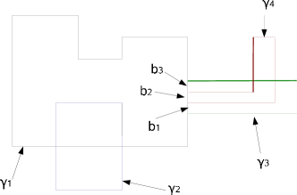
Figure 2: A contribution to the summation of Eq. (41) with $n=4$. Here we have: a bond with overlap of order 3, $b_{2}=\gamma_{1}\cap\gamma_{3}\cap\gamma_{4}$; two bonds with overlap of order 2, $b_{1}\cup b_{3}=\gamma_{1}\cap\gamma_{3}$; and all the other bonds with no overlap (order 1). Note that the multi-paths $\gamma_{1}$ and $\gamma_{2}$ intersect each other as geometrical objects but not as sets (for definition, a path $\gamma$ is the union of its bonds). The same observation holds for the multi-paths $\gamma_{3}\setminus(b_{1}\cup b_{2}\cup b_{3})$ and $\gamma_{4}\setminus b_{2}$.

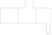
Figure 3: A chain of three connected planar multi-paths encapsulated in a larger planar path. The four multi-paths overlap each other only partially. The multi-paths in the figure are slightly shifted for visual convenience.

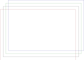
Figure 4: Schematic example of four completely overlapping planar multi-paths. The multi-paths in the figure are slightly shifted for visual convenience.

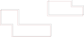
Figure 5: Schematic example of two couples of two completely overlapping planar multi-paths. The multi-paths in the figure are slightly shifted for visual convenience.

We find it useful to decompose the set of the four replica multi-paths of length $l^{\prime}\leq l$ as follows

$$\mathscr{E}_{4}(l)=\mathscr{E}_{4,4}(l)\cup\mathscr{E}_{2,4}(l)\cup\mathscr{R}_{4}(l),$$ (57)

where $\mathscr{E}_{4,4}(l)$ is the set of 4 coinciding multi-paths, i.e. the set of all one replica multi-paths, see Fig. 4; $\mathscr{E}_{2,4}(l)$ is the set of all multi-paths overlapping in couples (two to two), see Fig. 5; and $\mathscr{R}_{4}(l)$ is the rest, i.e. the set of all multi-paths in $\mathscr{E}_{4}(l)$ which overlap each other only partially, see Fig. 3.

In [1] we have shown that, when $D$ is large enough, in a $D$-dimensional hypercube lattice for any $l$ one has

$$\frac{|\mathscr{E}_{4,4}(l)|}{|\mathscr{E}_{2,4}(l)|}=O\left(\frac{1}{D-1}\right),\quad\frac{|\mathscr{R}_{4}(l)|}{|\mathscr{E}_{2,4}(l)|}=O\left(\frac{1}{D-1}\right).$$ (58)

In a $D$-dimensional hypercube lattice any vertex is crossed by $D$ axis, which can be seen as infinitely long non overlapping multi-paths. Equation (58) says that, for any $l$, when $D\to\infty$ the sets $\mathscr{R}_{4}(l)$ and $\mathscr{E}_{4,4}(l)$ can be completely neglected and the mapping becomes exact. The fact that Eq. (58) holds for any $l$ allowed to consider the mapping for all temperatures where the high temperature expansion converges, that is for all $\beta<\beta_{c}$. We want now to try to generalize Eq. (58) to arbitrary graphs. The idea is to observe that, even if the mean connectivity $\bar{k}$ is finite, as $l$ goes to infinity, Eq. (58) becomes true. However, as we shall show soon, for general graphs we cannot isolate the sets $\mathscr{E}_{2,4}$ and $\mathscr{E}_{4,4}$ because their union constitute the elements over which the summation runs. Let us observe that, if $\bar{k}$, the mean connectivity of a vertex is greater than 1, $\bar{k}>1$, we have that $C_{N}(l)$ grows exponentially in $l$. For the total number of simple (non multi) paths one has $c_{N}(l)\propto(\bar{k}-1)^{l}$ [17] but approximately this remains true also for the total number of multi-paths $C_{N}(l)=\mathrm{O}((\bar{k}-1)^{l})$. However, for what follows, we do not need the exact expression for $C_{N}(l)$. For our aims here, it is enough to keep in mind that $C_{N}(l)$ grows exponentially with $l$ according to some rate related to $\bar{k}$. For any graph and for large $l$ we have

$$|\mathcal{E}_{4,4}(l)|\propto C_{N}(l),$$ (59)

where we have used the fact that there is only one single way to overlap completely four multi-paths of length $l$. Similarly, for the set $\mathscr{R}_{4}(l)$ we have

$$|\mathcal{R}_{4}(l)|=\sum_{l^{\prime}}^{l}\sum\limits_{l_{1},l_{2},l_{3}:~{}l_{1}+l_{2}+l_{3}=l^{\prime}}C_{N}(l^{\prime})\propto l^{3}C_{N}(l)$$ (60)

where we have taken into account the degeneracy coming from the fact that given a multi-path of length $l^{\prime}$, we have to chose 3 multi-paths of lengths $l_{1},l_{2},l_{3}$ in all the possible ways such that be $l_{1}+l_{2}+l_{3}=l^{\prime}$. The set $|\mathscr{E}_{2,4}(l)|$ represents the total number of ways to arrange two multi-paths of length $l_{1}\leq l$ and $l_{2}\leq l$ which do not share any bond each other. Hence we have

$${|\mathscr{E}_{2,4}(l)|}\propto\left(C_{N}(l)\right)^{2}-C_{N}(l)$$ (61)

Therefore, from Eqs. (59) and (60) for large $l$ we arrive at the analogous of Eqs. (58)

$$\frac{|\mathscr{E}_{4,4}(l)|}{|\mathscr{E}_{2,4}(l)|}\propto\frac{1}{C_{N}(l)},\quad\frac{|\mathscr{R}_{4}(l)|}{|\mathscr{E}_{2,4}(l)|}\propto\frac{l^{3}}{C_{N}(l)},$$ (62)

implying that for sufficiently large lengths, we can neglect the contributions coming from the sets $\mathscr{E}_{4,4}$ and $\mathscr{R}_{4}$ so that, from Eq. (54), after a change of names, we are left with

$$P^{(4)}_{N} = 3\sum_{l_{1},l_{2},l^{(2)}}^{N}C_{N}(l_{1},l_{2};l^{(2)})\left(F^{\left(2\right)}_{b}\right)^{l_{1}+l_{2}-2l^{(2)}}\left(F^{\left(4\right)}_{b}\right)^{l^{(2)}},$$ (63)

where we have taken into account that we have 3 ways to couple 4 replicas of multi-paths overlapping two to two. Note that, as anticipated, we can neglect the contributions coming from the sets $\mathscr{E}_{4,4}$ and $\mathscr{R}_{4}$, but, in fact, , unlike a graph having $\bar{k}\to\infty$, as manifested by Eq.(63), we cannot isolate the sets $\mathscr{E}_{4,4}$ and $\mathscr{E}_{2,4}$. This problem will be analyzed in the second step of the proof.

Similarly, for $P^{(6)}$, one finds $|\mathscr{E}_{2,6}(l)|\propto\left(C_{N}(l)\right)^{3}$, $|\mathscr{E}_{4,6}(l)|\propto\left(C_{N}(l)\right)^{2}$, $|\mathscr{E}_{6,6}(l)|\propto C_{N}(l)$, and $|\mathscr{R}_{6}(l)|\propto l^{5}\left(C_{N}(l)\right)^{2}$, so that, after a change of names, we are left with

$$P^{(6)}_{N} = 15\sum_{l_{1},l_{2},l_{3},l^{(2)},l^{(3)}}^{N}C_{N}(l_{1},l_{2},l_{3};l^{(2)},l^{(3)})\left(F^{\left(2\right)}_{b}\right)^{l_{1}+l_{2}+l_{3}-2l^{(2)}-3l^{(3)}}$$ (64)

$$\times\left(F^{\left(4\right)}_{b}\right)^{l^{(2)}}\left(F^{\left(6\right)}_{b}\right)^{l^{(3)}},$$

where we have taken into account that we have $15=6!/2^{3}$ ways to couple 6 replicas of multi-paths two to two, but only one way to overlap the 6 replicas of multi-paths completely over the same single path. Generalizing to arbitrary $n$ we arrive at

$$P^{(2n)}_{N} = \frac{(2n)!}{2^{n}}\sum_{l_{1},\ldots,l_{n},l^{(2)},\ldots,l^{(n)}}^{N}C_{N}(l_{1},\ldots,l_{n},l^{(2)},\ldots,l^{(n)})$$ (65)

$$\times\left(F^{\left(2\right)}_{b}\right)^{l_{1}+\ldots+l_{n}-2l^{(2)}-\ldots-nl^{(n)}}\left(F^{\left(4\right)}_{b}\right)^{l^{(2)}}\cdots\left(F^{\left(2n\right)}_{b}\right)^{l^{(n)}}.$$

If we choose the delta plus minus measure $d\mu_{\pm}$

$$\frac{d\mu_{\pm}(J_{b})}{dJ_{b}}\equiv\frac{1}{2}\delta(J_{b}-J)+\frac{1}{2}\delta(J_{b}+J),$$ (66)

due to the property $\left(F^{\left(2n\right)}_{b}\right)=\left(F^{\left(2\right)}_{b}\right)^{n}$, and using $\sum_{l^{(2)}}C(l_{1},l_{2};l^{(2)})$ we get immediately that near the critical temperature

$$P^{(2n)}_{N\to\infty}=\left(P_{N\to\infty}\left(F_{b}^{(2)}\right)\right)^{n},\quad d\mu(J_{b})=d\mu_{\pm}(J_{b}).$$ (67)

8.1.2 Second step

We want now to show that for any symmetrical measure $d\mu$, if Eq. (10) (and then (45)) is satisfied, near the critical temperature it holds

$$P^{(2n)}_{N\to\infty}\propto\left(P_{N\to\infty}\left(F_{b}^{(2)}\right)\right)^{n}.$$ (68)

The idea of the proof is based on three key points. First, we use the fact that near the critical temperature only infinitely long multi-paths contribute to $P^{(n)}$. Second, we use our fundamental hypothesis (10). Third, we use the observation that, given two series $S=\sum_{l}a_{l}z^{l}$ and $S^{\prime}=\sum_{l}a_{l}b_{l}z^{l}$, if for $l\to\infty$, $b_{l}\to b$ with $0<|b|<\infty$, the two series have the same radius of convergence. Let us rewrite Eq. (63) as

$$P^{(4)}_{N} = 3\sum_{l_{1},l_{2},l^{(2)}}^{N}C_{N}(l_{1},l_{2};l^{(2)})\left(F^{\left(2\right)}_{b}\right)^{l_{1}+l_{2}}x_{b}^{l^{(2)}},$$ (69)

where

$$x_{b}(\beta)\equiv\frac{F^{\left(4\right)}_{b}}{\left(F^{\left(2\right)}_{b}\right)^{2}}.$$ (70)

Notice that, due to the Cauchy-Schwartz inequality, $x_{b}\geq 1$ and it is equal to 1 only for the delta plus-minus measure. To study the critical behavior of the system we need to know the singularities of $P^{(2n)}_{N}$ for $N\to\infty$. Let us now rewrite Eq. (69) as follows

$$P^{(4)}_{N} = 3\sum_{l_{1},l_{2}}^{N}C_{N}(l_{1},l_{2})B_{N}(l_{1},l_{2})\left(F^{\left(2\right)}_{b}\right)^{l_{1}+l_{2}},$$ (71)

where

$$B_{N}(l_{1},l_{2}) \equiv \frac{\sum_{l^{(2)}}^{\mathrm{min}(l_{1},l_{2})}C_{N}(l_{1},l_{2};l^{(2)})x_{b}^{l^{(2)}}}{\sum_{l^{(2)}}^{\mathrm{min}(l_{1},l_{2})}C_{N}(l_{1},l_{2};l^{(2)})}$$ (72)

$$= \sum_{l^{(2)}}^{\mathrm{min}(l_{1},l_{2})}\mathcal{P}_{N}(l_{1},l_{2};l^{(2)})x_{b}^{l^{(2)}}.$$

and in Eq. (72) we have made explicit in the sums the limit in $l^{(2)}$, $\mathrm{min}(l_{1},l_{2})$, above which $C_{N}(l_{1},l_{2};l^{(2)})$ becomes 0. Let us observe that in the $\lim_{l_{1},l_{2}\to\infty}~{}\lim_{N\to\infty}$, Eq. (72) becomes a power series in $l^{(2)}$ in powers of $x_{b}$ which, due to Eq. (45), has a non zero radius of convergence given by $\exp(a^{\prime})$. The given measure $d\mu$ belongs to some functional space $\mathcal{L}$ embedded with some distance $\|\cdot\|$. Let us now introduce in $\mathcal{L}$, the following set of measures

$$\mathcal{H}_{4}^{(\epsilon_{4})}=\left\{d\tilde{\mu}_{4}\in\mathcal{L}:\quad x_{b}(\beta)|_{d\tilde{\mu}_{4}}={\frac{F^{\left(4\right)}_{b}}{\left(F^{\left(2\right)}_{b}\right)^{2}}}|_{d\tilde{\mu}_{4}}<e^{\frac{1}{2}a^{\prime}-\epsilon_{4}},\forall\beta\right\},$$ (73)

with $0<\epsilon_{4}\ll a^{\prime}/2$ and let us define a measure $d\mu_{4}$ in such a way that

$$\|d\mu_{4}-d\mu\|=\inf\limits_{d\tilde{\mu}_{4}\in\mathcal{H}_{4}^{(\epsilon_{4})}}\|d\tilde{\mu}_{4}-d\mu\|.$$ (74)

One can look at the measure $d\mu_{4}$ as an “intermediate” measure between the given measure $d\mu$ which, in general, does not belong to the set $\mathcal{H}_{4}^{(\epsilon_{4})}$, and the plus-minus delta measure $d\mu_{\pm}$ which satisfies the condition for $\mathcal{H}_{4}^{(\epsilon_{4})}$. Note that $\mathcal{H}_{4}^{(\epsilon_{4})}$ is dense set. Equation (74) implies

$$x_{b}(\beta)|_{d\mu_{4}}<e^{\frac{1}{2}a^{\prime}},\quad\forall\beta.$$ (75)

In defining $\mathcal{H}_{4}^{(\epsilon_{4})}$ we have introduced a small parameter $\epsilon_{4}>0$ for having the above inequality strict, furthermore, for reasons will become clear later, we have introduced the space $\mathcal{H}_{4}^{(\epsilon_{4})}$ defined through the exponent $a^{\prime}/2$ rather than $a^{\prime}$. Therefore, for the modified measure $d\mu_{4}$, the power series (72) converges and we can analyze the $\lim_{l_{1},l_{2}\to\infty}~{}\lim_{N\to\infty}$ of $B_{N}(l_{1},l_{2})$, by switching the limit of the series with the series of the limit. As a result we see that for the modified measure $d\mu_{4}$ we have

$$\lim_{l_{1},l_{2}\to\infty}~{}\lim_{N\to\infty}B_{N}(l_{1},l_{2})|_{d{\mu}_{4}}=B_{4},\quad\forall\beta,$$ (76)

where $B_{4}=B_{4}(\beta)$ is a positive function of $\beta$ analytic for any values of $\beta$. Due to the fact that near the critical point only infinitely long multi-paths contribute to the series and by noting that $C_{N}(l_{1},l_{2})=C_{N}(l_{1})C_{N}(l_{2})$, by using Eq. (76) in Eq. (71) we get

$$\lim_{\beta\to\beta_{4}{-}}P^{(4)}_{N\to\infty}|_{d{\mu}_{4}} = \lim_{\beta\to\beta_{4}{-}}3B_{4}\left(P_{N\to\infty}\left(F_{b}^{(2)}\right)\right)^{2}|_{d{\mu}_{4}},$$ (77)

where $\beta_{4}$ is the inverse critical temperature of the related Ising model whose couplings, in terms of the high temperature expansion parameters $\tanh(\beta J^{(I)})$ are substituted by the terms $\left(F_{b}^{(2)}\right)|_{d{\mu}_{4}}$. This equation shows, in particular, that with the measure $d\mu_{4}$ the term $P^{(4)}$ is singular at the value $\beta_{4}$, i.e., the inverse critical temperature $\beta_{c}^{\mathrm{(SG)}}$ given by the Eq. (23) of the mapping.

Similarly, for $P^{(6)}$ from Eq. (64) we have

$$P^{(6)}_{N} = 15\sum_{l_{1},l_{2},l_{3},l^{(2)},l^{(3)}}^{N}C_{N}(l_{1},l_{2},l_{3};l^{(2)},l^{(3)})\left(F^{\left(2\right)}_{b}\right)^{l_{1}+l_{2}+l_{3}}x_{b}^{l^{(2)}}y_{b}^{l^{(3)}},$$ (78)

where $x_{b}$ is defined as in Eq. (70), whereas $y_{b}$ is defined as

$$y_{b}(\beta)\equiv\frac{F^{\left(6\right)}_{b}}{\left(F^{\left(2\right)}_{b}\right)^{3}}.$$ (79)

Notice that, due to the H$\ddot{o}$lder inequality, as $x_{b}$, also $y_{b}\geq 1$ and it is equal to 1 only for the delta plus-minus measure. We recall that $C_{N}(l_{1},l_{2},l_{3};l^{(2)},l^{(3)})$ represents the number of triples of multi-paths of length $l_{1},l_{2},l_{3}$ which share two to two and three to three $l^{(2)}$ and $l^{(3)}$ bonds, respectively. Let us rewrite Eq. (78) as follows

$$P^{(6)}_{N} = 15\sum_{l_{1},l_{2},l_{3}}^{N}C_{N}(l_{1},l_{2},l_{3})B_{N}(l_{1},l_{2},l_{3})\left(F^{\left(2\right)}_{b}\right)^{l_{1}+l_{2}+l_{3}},$$ (80)

where

$$B_{N}(l_{1},l_{2},l_{3}) \equiv \frac{\sum_{l^{(2)},l^{(3)}}^{\bar{l^{(2)}},\bar{l^{(3)}}}C_{N}(l_{1},l_{2},l_{3};l^{(2)},l^{(3)})x_{b}^{l^{(2)}}y_{b}^{l^{(3)}}}{\sum_{l^{(2)},l^{(3)}}^{\bar{l^{(2)}},\bar{l^{(3)}}}C_{N}(l_{1},l_{2},l_{3};l^{(2)},l^{(3)})}$$ (81)

$$= \sum_{l^{(2)},l^{(3)}}^{\bar{l^{(2)}},\bar{l^{(3)}}}\mathcal{P}_{N}(l_{1},l_{2},l_{3};l^{(2)},l^{(3)})x_{b}^{l^{(2)}}y_{b}^{l^{(3)}},$$

$$\bar{l^{(2)}}\equiv\mathrm{max}\{\mathrm{min}(l_{1},l_{2});\mathrm{min}(l_{1},l_{3});\mathrm{min}(l_{2},l_{3})\},$$ (82)

and

$$\bar{l^{(3)}}\equiv\mathrm{min}(l_{1},l_{2},l_{3}).$$ (83)

Now, by using standard probability arguments as shown in Appendix B, it is easy to see that the condition (45) ensures also

$$\mathcal{P}(l_{1},l_{2},l_{3};l^{(2)},l^{(3)})\leq(C^{\prime})^{2}\left[\frac{\left(l^{(2)}\right)^{2}+\left(l^{(3)}\right)^{2}}{2}\right]^{\frac{1}{2}}e^{-\frac{1}{2}a^{\prime}l^{(2)}-\frac{1}{2}a^{\prime}l^{(3)}}.$$ (84)

We find it convenient to observe that Eq. (84) in particular implies

$$\mathcal{P}(l_{1},l_{2},l_{3};l^{(2)},l^{(3)})<(C^{\prime})^{2}\mathrm{max}\{l^{(2)},l^{(3)}\}\frac{4}{{(\frac{3}{2})!}^{\frac{1}{2}}}e^{-\frac{1}{4}a^{\prime}l^{(2)}-\frac{1}{4}a^{\prime}l^{(3)}}.$$ (85)

Let us introduce the following set of measures

$$\mathcal{H}_{6}=\left\{d\tilde{\mu}_{6}\in\mathcal{L}:\quad\frac{F^{\left(4\right)}_{b}}{\left(F^{\left(2\right)}_{b}\right)^{2}}|_{d\tilde{\mu}_{6}}<e^{\frac{1}{4}a^{\prime}},\frac{F^{\left(6\right)}_{b}}{\left(F^{\left(2\right)}_{b}\right)^{3}}|_{d\tilde{\mu}_{6}}<e^{\frac{1}{4}a^{\prime}},\forall\beta\right\},$$ (86)

and let us define a modified measure $d\mu_{6}$ in such a way that

$$\|d\mu_{6}-d\mu\|=\inf\limits_{d\tilde{\mu}_{6}\in\mathcal{H}_{6}}\|d\tilde{\mu}_{6}-d\mu\|.$$ (87)

From Eq. (87) for the measure $d\mu_{6}$ we have that for any $\beta$, $x_{b}(\beta)|_{d{\mu}_{6}}<e^{a^{\prime}/4}$ and $y_{b}(\beta)|_{d{\mu}_{6}}<e^{a^{\prime}/4}$ so that, according to Eq. (85), for any $\beta$ the power series (81) converges and, as in the previous case, we can evaluate the $\lim_{N\to\infty}\lim_{l_{1},l_{2},l_{3}\to\infty}$ of $B_{N}(l_{1},l_{2},l_{3})$ by switching the limit of the series with the series of the limit obtaining

$$\lim_{l_{1},l_{2},l_{3}\to\infty}\lim_{N\to\infty}B_{N}(l_{1},l_{2},l_{3})|_{d{\mu}_{6}}=B_{6},$$ (88)

where $B_{6}=B_{6}(\beta)$ is a positive function of $\beta$ analytic for any values of $\beta$. Finally, by noting that $C_{N}(l_{1},l_{2},l_{3})=C_{N}(l_{1})C_{N}(l_{2})C_{N}(l_{3})$ from Eq. (80) we get

$$\lim_{\beta\to\beta_{6}{-}}P^{(6)}_{N\to\infty}|_{d{\mu}_{6}} = \lim_{\beta\to\beta_{6}{-}}15B_{6}\left(P_{N\to\infty}\left(F_{b}^{(2)}\right)\right)^{3}|_{d{\mu}_{6}},$$ (89)

where $\beta_{6}$ is the inverse critical temperature of the related Ising model whose couplings, in terms of the high temperature expansion parameters $\tanh(\beta J^{(I)})$, are substituted by the terms $\left(F_{b}^{(2)}\right)|_{d{\mu}_{6}}$. This equation shows, in particular, that with the measure $d\mu_{6}$ the term $P^{(6)}$ is singular at the value $\beta_{6}$, i.e., the inverse critical temperature $\beta_{c}^{\mathrm{(SG)}}$ given by the Eq. (23) of the mapping.

Equation (84) can be generalized to any integer $n$ (see Appendix B)

$$\mathcal{P}(l_{1},\ldots,l_{n};l^{(2)},\ldots,l^{(n)}) \leq (C^{\prime})^{n}\left[\frac{\left(l^{(2)}\right)^{n-1}+\ldots+\left(l^{(n)}\right)^{n-1}}{(n-1)!}\right]^{\frac{1}{n-1}}$$ (90)

$$\times e^{-\frac{1}{n-1}a^{\prime}l^{(2)}-\ldots-\frac{1}{n-1}a^{\prime}l^{(n)}}$$

which, for $n>1$, leads also to the generalization of Eq. (85)

$$\mathcal{P}(l_{1},\ldots,l_{n};l^{(2)},\ldots,l^{(n)}) < (C^{\prime})^{n}\mathrm{max}\{l^{(2)},\ldots,l^{(n)}\}\frac{n+1}{{(\frac{n}{2})!}^{\frac{1}{n-1}}}e^{-\frac{1}{2n}a^{\prime}l^{(2)}-\ldots-\frac{1}{2n}a^{\prime}l^{(n)}}.$$ (91)

Hence, for any $n>1$, by repeating the same argument followed for $P^{(4)}_{N\to\infty}|_{d{\mu}_{4}}$ and $P^{(6)}_{N\to\infty}|_{d{\mu}_{6}}$ we get

$$\lim_{\beta\to\beta_{2n}{-}}P^{(2n)}_{N\to\infty}|_{d{\mu}_{2n}} = \lim_{\beta\to\beta_{2n}{-}}\frac{(2n)!}{2^{n}}B_{2n}\left(P_{N\to\infty}\left(F_{b}^{(2)}\right)\right)^{n}|_{d{\mu}_{2n}},$$ (92)

where: $B_{2n}=B_{2n}(\beta)$ is an analytic function of $\beta$ for any $\beta$, $d{\mu}_{2n}$ is a modified measure defined as

$$\|d\mu_{2n}-d\mu\|=\inf\limits_{d\tilde{\mu}_{2n}\in\mathcal{H}_{2n}}\|d\tilde{\mu}_{2n}-d\mu\|,$$ (93)

with

$$\mathcal{H}_{2n}=\left\{d\tilde{\mu}_{2n}\in\mathcal{L}:\quad\frac{F^{\left(4\right)}_{b}}{\left(F^{\left(2\right)}_{b}\right)^{2}}|_{d\tilde{\mu}_{2n}},\ldots,\frac{F^{\left(2n\right)}_{b}}{\left(F^{\left(2\right)}_{b}\right)^{n}}|_{d\tilde{\mu}_{2n}}<e^{\frac{1}{2n}a^{\prime}}.\forall\beta\right\},$$ (94)

and $\beta_{2n}$ is the inverse critical temperature of the related Ising model whose couplings, in terms of the high temperature expansion parameters $\tanh(\beta J^{(I)})$, are substituted by the terms $\left(F_{b}^{(2)}\right)|_{d{\mu}_{2n}}$. This equation shows, in particular, that with the measure $d\mu_{2n}$ the term $P^{(2n)}$ is singular at the value $\beta_{2n}$, i.e., the inverse critical temperature $\beta_{c}^{\mathrm{(SG)}}$ given by the Eq. (23) of the mapping.

Let us define $\beta_{0}=\beta_{c}^{\mathrm{(SG)}}$, the solution of Eq. (23) of the mapping with the given measure $d\mu$. We have now to calculate the free energy density term $\varphi$, by using the replica trick relation (43) or, equivalently

$$\varphi=\lim_{n\rightarrow 0}\lim_{N\rightarrow\infty}\frac{P^{(2n)}-1}{2nN}.$$ (95)

From the structure of the generic set $\mathcal{H}_{2n}$ it is immediate to recognize that $\mathcal{H}_{4}\supset\mathcal{H}_{6}\supset\ldots\supset\mathcal{H}_{2n}$ and that for $n\to\infty$ $\mathcal{H}_{2n}\to\{d\mu_{\pm}\}$. However we are interested in the opposite limit $n\to 0^{+}$. Let us observe that Eqs. (91-94) allow to be analytically continued to any real $n\geq 0$, with the pre-factor $C^{n}(n+1)/((n/2)!^{1/(n-1)}\to 1$ as $n\to 0$. In this limit, the analytic continuation of the constrains in Eq. (94) brings to $\mathcal{H}_{2n}\to\mathcal{L}$ and Eq. (93) gives $d\mu_{2n}\to d\mu$ with respect to the functional distance $\|\cdot\|$. Therefore, for Eq. (95) we are free to calculate the limit as

$$\varphi=\lim_{n\rightarrow 0}\lim_{N\rightarrow\infty}\frac{P^{(2n)}_{N}-1}{2nN}=\lim_{n\rightarrow 0}\lim_{N\rightarrow\infty}\frac{P_{N}^{(2n)}|_{d\mu_{2n}}-1}{2nN}$$ (96)

and from Eq. (92), and by using $\lim_{\beta\to\beta_{0}}f(\beta)=\lim_{n\to 0}f(\beta_{2n})$, we finally get:

$$\lim_{\beta\to\beta_{0}{-}}\varphi=\lim_{\beta\to\beta_{0}{-}}\lim_{N\rightarrow\infty}\frac{\log\left(P_{N}\left(F_{b}^{(2)}\right)\right)}{N}=\lim_{\beta\to\beta_{0}{-}}\frac{1}{2}\varphi_{I}\left(F_{b}^{(2)}\right).$$ (97)

We stress that within the replica trick this proof is exact. With Eqs. (91-94) we have indeed found that there exists a succession of spaces $\mathcal{H}_{2n}$ where Eq. (92) holds with $B_{2n}$ finite and that this succession can be analytically continued to any real $n\geq 0$. It is important to note here that such a situation does not apply in a finite $D$-dimensional hypercube lattice. In fact, in this case the probability $\mathcal{P}(l_{1},l_{2};l)$ behaves in a completely different manner and cannot satisfy the condition (10). More precisely, in these “particular” graphs, for $D>1$, even if $C_{N}(l)$ still continues to have an exponential growth in $l$, $C_{N}(l)\sim(\bar{k}-1)^{l}$, with $\bar{k}-1=2D-1$, the probability $\mathcal{P}(l_{1},l_{2};l)$ remains concentrated to values of $l$ near to the given lengths $l_{1}$ and $l_{2}$. We can easily understand this last statement by looking at the case $D=1$. Even tough in this case $\bar{k}=2$, this example turns out to be quite instructive. In fact, in one dimension, for $\mathcal{P}(l_{1},l_{2};l)$ we have exactly

$$\mathcal{P}(l_{1},l_{2};l)=\left\{\begin{array}[]{c}1,\quad l=\mathrm{min}\{l_{1},l_{2}\},\\ 0,\quad\mathrm{otherwise}.\end{array}\right.$$ (100)

With such a probability, Eq. (72) gives $B_{N}(l_{1},l_{2})=x_{b}^{\mathrm{min}\{l_{1},l_{2}\}}$ so that for $l_{1},l_{2}\to\infty$ $B_{N}(l_{1},l_{2})$ diverges and Eq. (77) does not hold. For $D>1$ and finite, in general, it is very difficult to calculate the probability $\mathcal{P}(l_{1},l_{2};l)$, but, roughly speaking, a similar behavior is expected as well [18].

8.2 Proof for any measure

For a generic measure, i.e. also non symmetric, we have $F_{b}^{(m)}\neq 0$ also for $m$ odd so that for calculating $P^{(2n)}$, besides the terms obtained in the previous section, we have to add the contributions involving all the possible odd overlaps due to $m$-overlaps with $m\geq 1$. Let us define $\beta_{2n}$ as

$$\beta_{2n}=\mathrm{min}\{\beta^{\mathrm{(SG)}}_{2n},\beta^{\mathrm{(F/AF)}}_{2n}\},$$ (101)

where $\beta^{(\mathrm{SG})}_{2n}$ and $\beta^{(\mathrm{F/AF})}_{2n}$ are the inverse critical temperatures of of the related Ising model whose couplings, in terms of the high temperature expansion parameters $\tanh(\beta J^{(I)})$ are substituted by the terms $\left(F_{b}^{(2)}\right)|_{d{\mu}_{4n}}$ and $\left(F_{b}^{(1)}\right)|_{d{\mu}_{4n}}$, respectively. On the same line of the Step 2 of the proof, we have that the singular behavior of the terms $P^{(2n)}$ is described by

$$\lim_{\beta\to\beta_{2}{-}}P^{(2)}_{N\to\infty}|_{d{\mu_{4}}} = \lim_{\beta\to\beta_{2}{-}}\left(P_{N\to\infty}\left(F_{b}^{(2)}\right)\right)|_{d{\mu_{4}}}+$$ (102)

$$\lim_{\beta\to\beta_{2}{-}}3B_{4}\left(P_{N\to\infty}\left(F_{b}^{(1)}\right)\right)^{2}|_{d{\mu}_{4}},$$

$$\lim_{\beta\to\beta_{4}{-}}P^{(4)}_{N\to\infty}|_{d{\mu}_{8}} = \lim_{\beta\to\beta_{4}{-}}3B_{4}\left(P_{N\to\infty}\left(F_{b}^{(2)}\right)\right)^{2}|_{d{\mu}_{8}}+$$ (103)

$$\lim_{\beta\to\beta_{4}{-}}B_{8}\left(P_{N\to\infty}\left(F_{b}^{(1)}\right)\right)^{4}|_{d{\mu}_{8}},$$

$$\lim_{\beta\to\beta_{2n}{-}}P^{(2n)}_{N\to\infty}|_{d{\mu}_{4n}} = \lim_{\beta\to\beta_{2n}{-}}\frac{(2n)!}{2^{n}}B_{2n}\left(P_{N\to\infty}\left(F_{b}^{(2)}\right)\right)^{n}|_{d{\mu}_{4n}}+$$ (104)

$$\lim_{\beta\to\beta_{2n}{-}}B_{4n}\left(P_{N\to\infty}\left(F_{b}^{(1)}\right)\right)^{2n}|_{d{\mu}_{4n}},$$

where we have made use of the fact that $\mathcal{H}_{2n}\supset\mathcal{H}_{2n+2}$. By using Eq. (104), $\mathcal{H}_{2n}\to\mathcal{L}$ as $n\to 0^{+}$, and Eq. (95) we see that the upper critical surface is given by Eq. (22). Finally, the generalization to an arbitrary measure $d\mu_{b}$ which depends also on the bond $b\in\Gamma$ is straightforward: Eq. (104) has to be substituted with an analogous equation in which we have simply to replace $d\mu_{4n}$, $F_{b}^{(2)}$ and $F_{b}^{(1)}$ with the corresponding vectors $\{d\mu_{b}\}_{4n}$, $\{F_{b}^{(2)}\}$ and $\{F_{b}^{(1)}\}$, respectively.

9 The case of the measure $\mu_{\pm}$

In the previous section, we have proved the mapping in two steps, along the subsections 8.1.1 and 8.1.2. Unlike the second step, in the first step, the measure $d\mu$ does not play any role. However, from Eq. (67) we see that the measure $d\mu_{\pm}$ results to be a very special measure; in fact this equation says that if $d\mu=d\mu_{\pm}$, the mapping turns out to be exact even in finite dimension. In particular, in $D=2$ dimensions a phase transition should exist. This result seems to be in contradiction with the known fact, from numerical simulations, that in $D=2$ dimensions there is no phase transition. The paradox is explained by looking at the Step 2 of the proof. From this part of the proof it becomes clear that within the set of all the possible measures, the measure $d\mu_{\pm}$ constitutes a singular measure, being the unique for which Eq. (67) can be satisfied and, as soon as a measure $d\mu$ is even infinitesimally different from the measure $d\mu_{\pm}$, Eq. (67) cannot be satisfied; the given measure $d\mu$ may instead satisfy Eq. (68) but only in infinite dimensions. Therefore, within the set of all the measures, the measure $d\mu_{\pm}$ represents a singular measure for which there is an unstable phase transition with no physical counterpart. We recall that even in a numerical experiment it is impossible to represent exactly the singular measure $d\mu_{\pm}$. In fact, one can try to reproduce numerically such a distribution of bonds approximately by a smooth modification, but not exactly.

10 Nishimori law

Let us consider an arbitrary measure $d\mu$ independent on the bond $b$. From the equations of the mapping (20-24) we see that it may exist a tricritical point $\beta_{ct}=\beta_{c}^{(\mathrm{SG})}=\beta_{c}^{(\mathrm{F})}$ where the phases F, P and SG meet given by

$$\int d\mu\tanh^{2}(\beta_{ct}J_{b})=\int d\mu\tanh(\beta_{ct}J_{b}).$$ (105)

In the particular case of the measure

$$\frac{d\mu(J_{b})}{dJ_{b}}=p\delta(J_{b}-J)+(1-p)\delta(J_{b}+J),\qquad 0\leq p\leq 1,$$ (106)

Eq. (105) gives

$$\tanh(\beta_{ct}J)=2p-1.$$ (107)

From Eq. (107) we see that, as it must be, for any choice of $p$, the multicritical point F-P-SG belongs to the Nishimori line [19]. Equation (105) can be seen as a generalization of the Nishimori line to any measure.

Let us come back to the measure (106). The Nishimori theorems say also that, for any $p$, the internal energy along the Nishimori line $\tanh(\beta J)=2p-1$ is given by $E=-(NkJ/2)\tanh(\beta J)$ or, equivalently, the free energy is given by $-\beta F=(Nk/2)\log(2\cosh(\beta J))$, where $k$ is the mean connectivity, or coordination number. According to our definition of $\varphi$, Eq. (30), this implies that $\varphi=0$ along the Nishimori line. In the framework of the mapping this result can be checked from the fact that along the P-F and the P-SG lines $\varphi$ is given by $\varphi_{I}((2p-1)\tanh(\beta_{c}J))$ and $\varphi_{I}(\tanh^{2}(\beta_{c}J))/2$, respectively, so that on the multicritical point $\beta_{ct}$ it must be $\varphi_{I}((2p-1)\tanh(\beta_{c}J))=\varphi_{I}(\tanh^{2}(\beta_{c}J))/2$. From Eq. (107) we see that the only solution of this last equation can be only $\varphi=\varphi_{I}\equiv 0$ along all the upper critical line and, for continuity, in all the P region. By repeating this argument in the general case for an arbitrary measure $d\mu$ independent on $b$, and by using Eq. (105), we get

$$\varphi=\varphi_{I}\equiv 0,\quad\mathrm{in~{}the~{}P~{}region},$$ (108)

or equivalently

$$E=-\frac{Nk}{2}\int d\mu(J_{b})J_{b}\tanh(\beta J_{b}),\quad E_{I}=-\frac{Nk}{2}J^{(I)}\tanh(\beta J^{(I)}),\quad\mathrm{in~{}P}.$$ (109)

Notice that this result holds also for the related Ising model.

A further generalization can be also considered when the measure depends also on the bond $b$. From Eqs. (20-24) we see that the multicritical point $\beta_{ct}=\beta_{c}^{(\mathrm{SG})}=\beta_{c}^{(\mathrm{F/AF})}$ must satisfy the two following - possibly vectorial - equations

$$G_{I}\left(\left\{\int d\mu_{b}(J_{b})\tanh(\beta_{ct}J_{b})\right\}\right)=0,$$ (110)

and

$$G_{I}\left(\left\{\int d\mu_{b}(J_{b})\tanh^{2}(\beta_{ct}J_{b})\right\}\right)=0.$$ (111)

These equations may be regarded as the most general formulation of the Nishimori surface for models defined over graphs infinite dimensional in the broad sense. Here we use the term Nishimori surface, just to indicate a surface passing through the multicritical points (or even multicritical surfaces) and having the following property: as we change continously the parameters of the measures $\{d\mu_{b}\}$ as to approach a single measure $d\mu$ no longer dependent on the bond $b$, we approach the Nishimori line (105) for which Eqs. (108) and (109) hold.

We claim that Eq. (108) (or (109)) is the feature characterizing the models defined over graphs infinite dimensional in the broad sense: $\varphi$ (or $\varphi_{I}$) is zero not only along the Nishimori line, but over the whole P region.

Note however that there can be exceptions to the above rule for the graphs where the density free energy $f$ (and then also $\varphi_{I}$) does not exist in the proper sense. As mentioned in Sec. 4, this may happen in considering models over Husimi trees. Like in the Bethe lattices, in the Husimi trees, the thermodynamic limit of the density free energy does not exist. In these kind of models in fact, what is sensible is only the physics of the central spin: its magnetization and correlation functions obtained with recursive relations [20]. From these quantities one can then define the free energy a posteriori as done in [8]. It is possible to check that in a Bethe lattice one has however $\varphi_{I}\equiv 0$ in the P region. However, that does not happen in a Husimi tree (we have seen this for the model considered in [20]). Note that this is not in contradiction with the theorem of Nishimori. In fact, the Nishimori theorem, as well as our mapping, concerns, rigorously speaking, only “regular” models for which the free energy has some thermodynamic limit (see Eq. (6) of Ref. [19]). The models defined over Bethe lattices and Husimi trees therefore may, in general, not satisfy the Nishimori theorems. The fact that over Bethe lattices they still satisfy the Nishimori theorems is accidentally due to the tree-like structure of the Bethe lattices.

11 Conclusions

We have deepened concepts and claims already mentioned and used in the Refs. [1] and [4] and we have provided a complete proof of the mapping for general graphs. The condition for the mapping to become exact for these graphs is not exactly what claimed in [1], where we simply required a decay of $p(l)$ to 0 for $l$ going to infinity (such a requirement is in fact only a necessary condition if $p(l)$ is a probability). The mapping becomes exact whenever $p(l)$ decays at least exponentially or, for the most general case (even if the limit $p(l)$ does not exist), when Eq. (10) is satisfied. As Eq. (10) is satisfied we say that the graph is infinite dimensional in the broad sense. The use of this expression is motivated by the fact Eq. (10) implies the infinite dimensionality in the traditional sense (see Eqs. (12) and 15) but not vice-versa. In fact, this non equivalence represents an interesting point, since there exist graphs where the tree-like approximation cannot be applied but, nevertheless, they are infinite dimensional in the broad sense. Also from this observation, it should be clear that the proof of the mapping, far from being simple, is not based on some local analysis of the graph, but on the key requirement expressed by Eq. (10), which represents a global information; a crucial feature in spin glass models. Note that, along the proof, no ansatz, such as the replica symmetric one, has been used.

The powerful of the mapping in respect of its simplicity and generality has still to be explored. Applications of the mapping to random graphs not yet considered in Ref. [4] and its extensions to include graphs with constrains (complex networks) and others non Ising models are the object of present and future investigations.

Appendix A A sufficient condition

The mapping becomes exact under the condition (45) for $\mathcal{P}(l_{1},l_{2};l)$, the probability that two infinitely long - multi-paths - arbitrarily chosen overlap for $l$ bonds. The probability $\mathcal{P}(l_{1},l_{2};l)$ is however an awkward quantity of not direct access. We are more interested in using the probability $p(l_{1},l_{2};l)$ introduced in Sec. 3 that two infinitely long - simple - paths overlap for $l$ bonds. In fact, unlike $\mathcal{P}(l_{1},l_{2};l)$, $p(l_{1},l_{2};l)$ concerns only simple connected paths (mono-component) and it is therefore a suitable quantity of easier practical access. We want now to find a sufficient condition for Eqs. (45) to be satisfied in terms of $p(l_{1},l_{2};l)$. We will prove that the exponential decaying upper bound for $p(l_{1},l_{2};l)$ implies that of $\mathcal{P}(l_{1},l_{2};l)$ with a little but finite diminishing of the exponent.

Given $l_{1}$, $l_{2}$ and $l\leq\mathrm{min}\{l_{1},l_{2}\}$, let $\mathcal{P}_{N}(l_{1},l_{2};l|k)$ be the conditional probability that two multi-paths of length $l_{1}$ and $l_{2}$ overlap for $l$ bonds along $k$ common portions of $k$ simple multi-paths of the first and second multi-path. The $k$ portions belong to a common multi-path of length $l$.

For definition of $\mathcal{P}_{N}(l_{1},l_{2};l)$ we have

$$\mathcal{P}_{N}(l_{1},l_{2};l)=\sum_{k}^{l}\mathcal{P}_{N}(l_{1},l_{2};l|k)\mathcal{P}_{N}(l;k),$$ (112)

where $\mathcal{P}_{N}(l;k)$ is the probability that the common multi-path of length $l$ is constituted by $k$ components (or simple paths).

Let us indicate with $\xi_{1},\ldots,\xi_{k}$ the numbers of two to two shared bonds along the $k$ common portions of the $k$ simple multi-paths of the two multi-paths. Looking at the $\xi$’s as random variables, we have

$$\mathcal{P}_{N}(l_{1},l_{2};l|k)=\sum_{x_{1}+\ldots+x_{k}=l}\mathcal{P}_{N}(l_{1},l_{2};\xi_{1}=x_{1},\ldots,\xi_{k}=x_{k}),$$ (113)

where $\mathcal{P}_{N}(l_{1},l_{2};\xi_{1}=x_{1},\ldots,\xi_{k}=x_{k})$ is the probability that two multi-paths of lengths $l_{1}$ and $l_{2}$ overlap two to two for $x_{1},\ldots,x_{k}$ bonds along the $k$ common regions of the $k$ simple paths. Note that, for definition of a path, the $k$ components cannot share common bond each other. In fact we can say more. We are interested in the limit $\lim_{l\to\infty}\lim_{l_{1},l_{2}\to\infty}$. In words this means that we keep $l$ fixed and look at the situation in which the total lengths $l_{1}$ and $l_{2}$ of the two multi-paths become larger and larger. In this limit the $k$ portions become farer and farer islands of fixed size. Therefore, in the limit of interest, we can approximate the random variables $\xi_{1},\ldots,\xi_{k}$ as independent so that the probability $\mathcal{P}_{N}(l_{1},l_{2};\xi_{1}=x_{1},\ldots,\xi_{k}=x_{k})$ factorizes as

$$\mathcal{P}_{N}(l_{1},l_{2};\xi_{1}=x_{1},\ldots,\xi_{k}=x_{k})=p_{N}(l_{1}^{\prime},l_{2}^{\prime};x_{1})\cdots p_{N}(l_{1}^{\prime},l_{2}^{\prime};x_{k}),$$ (114)

where $l_{1}^{\prime}$ and $l_{2}^{\prime}$ are rescaled lengths of the order of $l_{1}^{\prime}=\mathop{O}(l_{1}/k)$ and $l_{2}^{\prime}=\mathop{O}(l_{2}/k)$. We observe that in the limit $l_{1},l_{2}\to\infty$ we have also $l_{1}^{\prime},l_{2}^{\prime}\to\infty$.

In the limit $l\to\infty$, we are allowed, for the sake of simplicity, to take the variable $l$ in the continuum. Note that in such a case we have to consider the following substitution rules

$$\sum_{l}\Rightarrow\int dl$$ (115)

$$\lim_{l_{1},l_{2}\to\infty}C_{l_{1},l_{2}}=\frac{e^{a}-1}{e^{a}}\Rightarrow\lim_{l_{1},l_{2}\to\infty}C_{l_{1},l_{2}}=a$$ (116)

$$\sum_{x_{1}+\ldots+x_{k}=l}\Rightarrow\int dx_{1}\cdots dx_{k}\delta({x_{1}+\ldots+x_{k}-l}).$$ (117)

The great simplification in considering continuum variables stands in the last rule. In fact, we are able to calculate easily the above multi integral as

$$\int_{0}^{l}dx_{1}\cdots dx_{k}\delta({x_{1}+\ldots+x_{k}-l})=\frac{l^{k-1}}{(k-1)!}.$$ (118)

If we assume now the exponential decay (10) for $p(l_{1},l_{2};l)$, by using Eqs. (114) and (118), Eq. (113) becomes

$$\mathcal{P}_{N}(l_{1},l_{2};l|k)\leq C^{k}e^{-al}\frac{l^{k-1}}{(k-1)!}.$$ (119)

Taking into account the second of the Eqs. (115), in the limit $l_{1},l_{2}\to\infty$ the normalization of the r.h.s. of Eq. (119) can be checked immediately by using

$$\int_{0}^{\infty}e^{-al}l^{n}=\frac{n!}{a^{n}}.$$ (120)

The evaluation of the probability $\mathcal{P}_{N}(l;k)$ for having $k$ components (islands) of total length $l$, can be easily obtained along the same line with the use of Eq. (118). In fact, since, given $l$, all the components $x_{1},\ldots,x_{k}$ are equiprobable, the only constrain for the random variable $k$ is that be $x_{1}+\ldots+x_{k}=l$. So that, in the continuum for $l$, from Eq. (118) we get

$$\mathcal{P}_{N}(l;k)=\frac{l^{k-1}}{(k-1)!}e^{-l},$$ (121)

where the factor $\exp(-l)$ comes from the normalization constant. Equation (121) could be derived also by observing that, given $l$, $k$ describes the number of jumps inside the interval $[0,l]$ of a homogeneous jump process which, in correspondence of any bond $b$ of length 1, may or may not to jump to another island, so that $k$ is distributed according to a Poisson distribution with rate $\rho=1$.

Now, from Eqs. (112), (119) and (121), by passing in the continuum also for $k$ and by using the Stirling approximation we have

$$\mathcal{P}_{N}(l_{1},l_{2};l)\leq\int_{0}^{l}dke^{\psi(k)}\frac{1}{2\pi(k-1)},$$ (122)

where we have introduced the non smooth part of the integrand

$$\psi(k)=-al-l+k\log(C)+2(k-1)\log(l)-2[(k-1)\log(k-1)-(k-1)].$$ (123)

By a saddle point calculation in $k$ we get, $\partial_{k}\psi(k)=0$ for $k^{\mathrm{sp}}=l\sqrt{C}$, and using $\partial_{k}^{2}\psi(k)|_{k^{\mathrm{sp}}}=-2/(l\sqrt{C})$, for large $l$ we arrive at

$$\mathcal{P}_{N}(l_{1},l_{2};l)\leq e^{-l(a-2\sqrt{C}+1)}\frac{1}{(2\pi)^{1/2}C^{1/4}\sqrt{l}}.$$ (124)

Finally, by using $C=a$ we have

$$\mathcal{P}_{N}(l_{1},l_{2};l)\leq e^{-l(a-2\sqrt{a}+1)}\frac{1}{(2\pi)^{1/2}a^{1/4}\sqrt{l}}.$$ (125)

Since $a^{\prime}\equiv a-2\sqrt{a}+1>0$ for any real $a$, we have proved that an exponential decay in $l$ for $p_{N}(l_{1},l_{2};l)$ implies always an exponential decay for $\mathcal{P}_{N}(l_{1},l_{2};l)$. It is interesting to observe that the rate of decay of the latter is diminished by the term $2\sqrt{a}-1$, which is positive for $a>1/4$.

Appendix B Inequalities

Equation (84) can be proved as follows. If $\mathcal{P}$ is some probability acting on sets $A_{1},\ldots,A_{n}$, one has

$$\mathcal{P}(A_{1}\cap\ldots\cap A_{n})\leq\left(\mathcal{P}(A_{1})\cdots\mathcal{P}(A_{n})\right)^{\frac{1}{n}},$$ (126)

so that for $\mathcal{P}(l_{1},l_{2},l_{3};l^{(2)},l^{(3)})$ we have

$$\mathcal{P}(l_{1},l_{2},l_{3};l^{(2)},l^{(3)})\leq\left(\mathcal{P}^{(2)}(l_{1},l_{2},l_{3};l^{(2)})\mathcal{P}^{(3)}(l_{1},l_{2},l_{3};l^{(3)})\right)^{\frac{1}{2}},$$ (127)

where, for $m\leq n$, we have introduced the probabilities $\mathcal{P}^{(m)}(l_{1},\ldots,l_{n};l^{(m)})$ for having a total of $l^{(m)}$ $m$-overlaps among the $n$ paths. So, the first factor in the rhs of Eq. (127) represents the probability for having a 2-overlap $l^{(2)}$ among a triplet of multi-paths of lengths $l_{1},l_{2},l_{3}$, whereas the second factor represents the probability for having a 3-overlap $l^{(3)}$ among the triplet.

On the same line of what we have seen in the Appendix A, we observe that, if $\xi_{12}$, $\xi_{13}$ and $\xi_{23}$, are the random variables associated with the total 2-overlap between the multi-paths 1 and 2, the multi-paths 1 and 3, and the multi-paths 2 and 3, respectively, we can decompose the probability $\mathcal{P}(l_{1},l_{2},l_{3};l^{(2)})$ as follows

$$\mathcal{P}_{N}^{(2)}(l_{1},l_{2},l_{3};l^{(2)})=\sum_{x_{12}+x_{13}+x_{23}=l^{(2)}}\mathcal{P}_{N}^{(2)}(l_{1},l_{2},l_{3};\xi_{12}=x_{12},\xi_{13}=x_{13},\xi_{23}=x_{23}).$$ (128)

On the other hand, in the limit $\lim_{l\to\infty}\lim_{l_{1},l_{2},l_{3}\to\infty}$, we can apply the same argument we have used in the Appendix A: the three families of regions between the multi-paths 1 and 2, 1 and 3, and 2 and 3, become infinitely far in this limit, so that the respective random variables $\xi_{12}$, $\xi_{13}$ and $\xi_{23}$ become independent and distributed according to the exponential decay (10). Hence, after using Eq. (118) we are left with

$$\mathcal{P}^{(2)}(l_{1},l_{2},l_{3};l^{(2)})\leq(C^{\prime})^{3}e^{-a^{\prime}l^{(2)}}\frac{\left(l^{(2)}\right)^{2}}{2},$$ (129)

where we have used Eq. (45).

Concerning the second factor, we simply observe that $l^{(3)}$ stands for a 3-overlap, therefore, by using the elementary inequality

$$\mathcal{P}(A\cap B\cap C)\leq\mathcal{P}(A\cap B),$$ (130)

we get

$$\mathcal{P}^{(3)}(l_{1},l_{2},l_{3};l^{(3)})\leq\mathcal{P}^{(2)}(l_{1},l_{2},l_{3};l^{(3)}).$$ (131)

By using Eqs. (127-130)) Eq. (84) is proved.

Similarly, for the general case, the analogous of Eq. (129) becomes

$$\mathcal{P}^{(2)}(l_{1},\ldots,l_{n};l^{(2)})\leq(C^{\prime})^{n}e^{-a^{\prime}l^{(2)}}\frac{\left(l^{(2)}\right)^{n-1}}{(n-1)!},$$ (132)

and, for any $2\leq m\leq n$, the analogous of Eq. (131) becomes

$$\mathcal{P}^{(m)}(l_{1},\ldots,l_{n};l^{(m)})\leq\mathcal{P}^{(2)}(l_{1},\ldots,l_{n};l^{\prime(2)}).$$ (133)

By using Eqs. (127), (132)) and (133), Eq. (90) is proved.

References

References

- [1] M. Ostilli, J. Stat. Mech. P10004 (2006).
- [2] Sherrington D and Kirkpatrick S, 1975 Phys. Rev. Lett. 35, 1792
- [3] Mezard M, Parisi G, Virasoro M A, 1987 Spin Glass Theory and Beyond (Singapore: World Scientific)
- [4] M. Ostilli, J. Stat. Mech. P10005 (2006).
- [5] More precisely, given a graph, the Bethe-Peierls approximation is exact when the corresponding factor graph is a tree. When in the factor graph there are loops, the Bethe-Peierls approach gives good results provided the length of the loops is sufficiently large (for example when the length scales as ), whereas, in the presence of short loops, corrections to the Bethe-Peierls approach may be important. Systematic corrections to the Bethe-Peierls approximation have been recently rigorously established in [6] and [7].
- [6] G. Parisi and F. Slanina, J. Stat. Mech. L02003 (2006).
- [7] M. Chertkov and V. Y Chernyak, J. Stat. Mech. P06009 (2006).
- [8] Baxter R J, 1982 Exact Solved Models in Statistical Mechanics (London: Academic Press).
- [9] M. Ostilli, in preparation. Note however that in part this assertion can be easily derived by looking at [4].
- [10] See Sec. 2 of: Mezard M and Parisi G, 2001 Eur. Phys. J. B 20 217-233
- [11] Dorogovtsev S N, Mendes J F F, 2003 Evolution of Networks (University Press: Oxford)
- [12] S.N. Dorogovtsev, J.F.F. Mendes, and A.N. Samukhin, 2003 Nucl. Phys. B 666, 396-416
- [13] S.N. Dorogovtsev and A.N. Samukhin, 2003 Phys. Rev. E 67, 037103 1-4
- [14] Benettin G, Gallavotti G, Jona-Lasinio G, Stella A L, 1973 Commun. Math. Phys. 30 45-54
- [15] C. Domb, Advan. Phys. 9, Nos. 34 and 35 (1960).
- [16] Van Hemmen J L and Palmer R G, 1979 J. Phys. A: Math Gen. 12 563-580
- [17] Fisher M and Gaunt D, 1964 Phys. Rev. 1A 133 224
- [18] I am in debt with F. Cesi for an illuminating discussion about this argument.
- [19] H. Nishimori, 1980 J. Phys. C: Solid St. Phys., 13, 4071.
- [20] M. Ostilli, F. Mukhamedov, J. F. Mendes, cond-math/0611654. In this manuscript we provide a mere application of the equation of the mapping regardless of the fact that, as stressed, the free energy for models defined over a Husimi tree, does not exist and the mapping here, rigorously speaking, cannot be applied.