Affine Buildings and Tropical Convexity

Abstract.

The notion of convexity in tropical geometry is closely related to notions of convexity in the theory of affine buildings. We explore this relationship from a combinatorial and computational perspective. Our results include a convex hull algorithm for the Bruhat–Tits building of $\operatorname{SL}_{d}(K)$ and techniques for computing with apartments and membranes. While the original inspiration was the work of Dress and Terhalle in phylogenetics, and of Faltings, Kapranov, Keel and Tevelev in algebraic geometry, our tropical algorithms will also be applicable to problems in other fields of mathematics.

1. Introduction

Buildings were initially introduced by Tits [24] to provide a common geometric framework for all simple Lie groups, including those of exceptional type. The later work of Bruhat and Tits [5] showed that buildings are fundamental in a much wider context, for instance, for applications in arithmetic algebraic geometry. Among the affine buildings, the key example is the Bruhat–Tits building $\mathcal{B}_{d}$ of the special linear group $\operatorname{SL}_{d}(K)$ over a field $K$ with a discrete non-archimedean valuation. An active line of research explores compactifications of the building $\mathcal{B}_{d}$; for example, see Kapranov [16] and Werner [25, 26].

Our motivation to study affine buildings stems from the connection to biology which was proposed in Andreas Dress’ 1998 ICM lecture The tree of life and other affine buildings [9]. Dress and Terhalle [8] introduced valuated matroids as a combinatorial approximation of the building $\mathcal{B}_{d}$, thereby generalizing the familiar one-dimensional picture of an infinite tree for $d=2$. In Section 4 we shall see that valuated matroids are equivalent to the matroid decompositions of hypersimplices of Kapranov [16, Definition 1.2.17], to the tropical linear spaces of Speyer [22], and to the membranes of Keel and Tevelev [17]. The latter equivalence, shown in [17, Theorem 4.15], will be revisited in Theorem 18 below.

We start out in Section 2 with a brief introduction to the Bruhat–Tits building $\mathcal{B}_{d}$ and to the notion of convexity in $\mathcal{B}_{d}$ which appears in work of Faltings [10]. For sake of concreteness we take $K$ to be the field $\mathbb{C}(\!(z)\!)$ of formal Laurent series with complex coefficients. Our discussion revolves around the algorithmic problem of computing the convex hull of a finite set of points in the building $\mathcal{B}_{d}$. Here each point is a lattice which is represented by an invertible $d\times d$-matrix with entries in $K=\mathbb{C}(\!(x)\!)$. Our solution to this problem involves identifying their convex hull in $\mathcal{B}_{d}$ with a certain tropical polytope.

Tropical convexity was introduced by Develin and Sturmfels [7]. Tropical polytopes are certain contractible polytopal complexes which are dual to the regular polyhedral subdivisions of the product of two simplices. A review of tropical convexity will be given in Section 4, along with some new results, extending a formula of Ardila [3], which characterize the nearest point projection onto a tropical polytope. In Section 4, we introduce tropical linear spaces, we represent them as tropical polytopes, and we identify them with membranes in $\mathcal{B}_{d}$. This allows us in Section 5 to reduce convexity in $\mathcal{B}_{d}$ to tropical convexity. In addition to our convex hull algorithm, we also study the related problems of intersecting apartments or, more generally, membranes. We prove the following result:

Theorem 1.

The min- and max-convex hulls of a finite set of lattices in $\mathcal{B}_{d}$ coincides with the standard triangulation of a tropical polytope in a suitable membrane.

This is stated more precisely in Proposition 22. New contributions made by this paper include the triangulation of tropical polytopes in Theorem 11, the formulas for projecting onto tropical linear spaces in Theorem 15, a combinatorial proof for the Keel-Tevelev bijection in Theorem 18, and, most important of all, the algorithms in Sections 5 and 6.

Acknowledgments: Michael Joswig was partially supported by Deutsche Forschungsgemeinschaft (FOR 565 Polyhedral Surfaces). Bernd Sturmfels was partially supported by the National Science Foundation (DMS-0456960), and Josephine Yu was supported by a UC Berkeley Graduate Opportunity Fellowship and by the IMA in Minneapolis.

2. The Bruhat–Tits building of $\operatorname{SL}_{d}(K)$

We review basic definitions concerning Bruhat–Tits buildings, following the presentations in [17, 18]. The most relevant section in the monograph by Abramenko and Brown is [1, §6.9]. Let $R=\mathbb{C}[\![z]\!]$ be the ring of formal power series with complex coefficients. Its field of fractions is the field $K=\mathbb{C}(\!(z)\!)$ of formal Laurent series with complex coefficients. Taking the exponent of the lowest term of a power series defines a valuation $\operatorname{val}:K^{*}\rightarrow\mathbb{Z}$. Note that $R$ is the subring of $K$ consisting of all field elements $c$ with $\operatorname{val}(c)\geq 0$. What follows is completely general and works for other fields with a non-archimedean discrete valuation, notably the $p$-adic numbers, but to keep matters most concrete we fix $K=\mathbb{C}(\!(z)\!)$. We extend the valuation to $K$ by setting $\operatorname{val}(0)=\infty$. If $M$ is a matrix over $K$ then $\operatorname{val}(M)$ denotes the matrix over $\mathbb{Z}\cup\{\infty\}$ whose entries are the values of the entries of $M$.

The vector space $K^{d}$ is a module over the ring $R$. A lattice in $K^{d}$ is an $R$-submodule generated by $d$ linearly independent vectors in $K^{d}$. Each lattice $\Lambda$ is represented as the image of a matrix $M$ with $d$ rows and $\geq d$ columns, with entries in $K$, having rank $d$. Two lattices $\Lambda_{1},\Lambda_{2}\subset K^{d}$ are equivalent if $c\Lambda_{1}=\Lambda_{2}$ for some $c\in K^{*}$. Two equivalence classes of lattices are called adjacent if there are representatives $\Lambda_{1}$ and $\Lambda_{2}$ such that $z\Lambda_{2}\subset\Lambda_{1}\subset\Lambda_{2}$.

The Bruhat–Tits building of $\operatorname{SL}_{d}(K)$ is the flag simplicial complex $\mathcal{B}_{d}$ whose vertices are the equivalence classes of lattices in $K^{d}$ and whose edges are the adjacent pairs of lattices. Being a flag simplicial complex means that a finite set of vertices forms a simplex if and only if any two elements in that set form an edge. The link of any lattice $\Lambda$ in $\mathcal{B}_{d}$ is isomorphic to the simplicial complex of all chains of subspaces in $\mathbb{C}^{d}=\Lambda/z\Lambda$. Thus the simplicial complex $\mathcal{B}_{d}$ is pure of dimension $d-1$, but it is not locally finite, since the residue field is $\mathbb{C}$. Our objective is to identify finite subcomplexes with a nice combinatorial structure which is suitable for reducing computations in $\mathcal{B}_{d}$ to tropical geometry.

If $\Lambda_{1}$ and $\Lambda_{2}$ are lattices then their $R$-module sum $\Lambda_{1}+\Lambda_{2}$ and their intersection $\Lambda_{1}\cap\Lambda_{2}$ are also lattices. These two operations give rise to two different notions of convexity on the Bruhat–Tits building $\mathcal{B}_{d}$. We say that a set $\mathcal{M}$ of lattices in $\mathcal{B}_{d}$ is max-convex if the set of all representatives for lattices in $\mathcal{M}$ is closed under finite $R$-module sums. We call $\mathcal{M}$ min-convex if that set is closed under finite intersections. If $\mathcal{L}$ is any subset of $\mathcal{B}_{d}$ then its max-convex hull $\operatorname{maxconv}(\mathcal{L})$ is the set of all lattices $\Lambda$ in $K^{d}$ such that $\Lambda$ is the $R$-module sum of finitely many lattices in $\mathcal{L}$. Similarly, the min-convex hull $\operatorname{minconv}(\mathcal{L})$ is the set of all lattices $\Lambda$ in $K^{d}$ such that $\Lambda$ is the intersection of finitely many lattices in $\mathcal{L}$. These notions of convexity give rise to the following problem in computational algebra:

Computational Problem A. Let $M_{1},\ldots,M_{s}$ be invertible $d\times d$-matrices with entries in $K=\mathbb{C}(\!(z)\!)$, representing lattices $\Lambda_{i}=\operatorname{image}_{R}(M_{i})$ in $K^{d}$. Compute both the min-convex hull and the max-convex hull of the lattices $\Lambda_{1},\ldots,\Lambda_{s}$ in the Bruhat–Tits building $\mathcal{B}_{d}$.

The duality functor $\operatorname{Hom}_{R}(\,\,\cdot\,\,,R)$ reduces a min-convex hull computation to a max-convex hull computation and vice versa. Given any lattice $\Lambda$, we write $\,\Lambda^{*}=\operatorname{Hom}_{R}(\Lambda,R)\,$ for the dual lattice. Any $R$-module homomorphism $\Lambda\rightarrow R$ extends uniquely to a $K$-vector space homomorphism $K^{d}\rightarrow K$. Hence the free $R$-module $\Lambda^{*}$ can be considered as a lattice in the dual vector space $(K^{d})^{*}=\operatorname{Hom}_{R}(K^{d},K)$, consisting of those elements that send $\Lambda$ into $R$. For any unit $c\in K^{*}$, we have $\,(c\Lambda)^{*}=\frac{1}{c}(\Lambda^{*})$. Since duality is inclusion-reversing, i.e. $\Lambda_{1}\subset\Lambda_{2}$ implies $\Lambda_{2}^{*}\subset\Lambda_{1}^{*}$, it respects equivalence of lattices and adjacency of vertices in the building $\mathcal{B}_{d}$. Moreover, duality switches sums and intersections:

Lemma 2.

For any two lattices $\Lambda_{1},\Lambda_{2}$ in $K^{d}$, we have $\,(\Lambda_{1}+\Lambda_{2})^{*}\,=\,\Lambda_{1}^{*}\cap\Lambda_{2}^{*}\,$ in $\,(K^{d})^{*}$.

Proof.

The inclusion “$\subseteq$” is given by restricting any ring homomorphism $\,\phi:\Lambda_{1}+\Lambda_{2}\rightarrow R\,$ to $\Lambda_{1}$ and to $\Lambda_{2}$, respectively. The reverse inclusion “$\supseteq$” is given by identifying $\,\phi\in\Lambda_{1}^{*}\cap\Lambda_{2}^{*}\,$ with the map $f_{1}+f_{2}\mapsto\phi(f_{1})+\phi(f_{2})$ where $f_{i}\in\Lambda_{i}$. ∎

It is known that both the max-convex hull and the min-convex hull of $\Lambda_{1},\ldots,\Lambda_{s}$ are finite simplicial complexes of dimension $\leq d-1$. This finiteness result is attributed by Keel and Tevelev [17, Lemma 4.11] to Faltings’ paper on matrix singularities [10].

Our usage of the prefixes “min” and “max” for convexity in $\mathcal{B}_{d}$ is consistent with the alternative representation of the Bruhat–Tits building in terms of additive norms on $K^{d}$. An additive norm is a map $N:K^{d}\rightarrow\mathbb{R}\cup\{\infty\}$ which satisfies the following three axioms:

1. $N(c\cdot f)=\operatorname{val}(c)+N(f)$ for any $c\in K$ and $f\in K^{d}$,

2. $N(f+g)\geq\min(N(f),N(g))$ for any $f,g\in K^{d}$,

3. $N(f)=\infty$ if and only if $f=0$.

We say that $N$ is an integral additive norm if $N$ takes values in $\mathbb{Z}\cup\{\infty\}$.

There is a natural bijection between lattices in $K^{d}$ and integral additive norms on $K^{d}$. Namely, if $N$ is an integral additive norm then its lattice is $\,\Lambda_{N}=\{f\in K^{d}:N(f)\geq 0\}$. Conversely, if $\Lambda$ is any lattice in $K^{d}$ then its additive norm $N_{\Lambda}$ is given by

(1) $$N_{\Lambda}(f)\ :=\ \max\left\{\,u\in\mathbb{Z}\vphantom{z^{-u}f\in\Lambda}\,:\,\vphantom{u\in\mathbb{Z}}z^{-u}f\in\Lambda\,\right\}\ =\ \min(\operatorname{val}(M^{-1}f))\,,$$

where $M$ is a $d\times d$-matrix whose columns form a basis for $\Lambda$. This bijection induces a homeomorphism between the space of all additive norms (with the topology of pointwise convergence) and the space underlying the Bruhat–Tits building $\mathcal{B}_{d}$. In other words, non-integral additive norms can be identified with points in the simplices of $\mathcal{B}_{d}$.

If $\Lambda_{1}$ and $\Lambda_{2}$ are lattices then the additive norm corresponding to the intersection $\Lambda_{1}\cap\Lambda_{2}$ is the pointwise minimum of the two norms:

$$N_{\Lambda_{1}\cap\Lambda_{2}}\quad=\quad\min(N_{\Lambda_{1}},N_{\Lambda_{2}})\,.$$

The pointwise maximum of two additive norms is generally not an additive norm. We write $\overline{\max}(N_{\Lambda_{1}},N_{\Lambda_{2}})$ for the smallest norm which is pointwise greater than or equal to $\max(N_{\Lambda_{1}},N_{\Lambda_{2}})$. Then we have

$$N_{\Lambda_{1}+\Lambda_{2}}\quad=\quad\overline{\max}(N_{\Lambda_{1}},N_{\Lambda_{2}})\,.$$

Our two notions of convexity on $\mathcal{B}_{d}$ correspond to the $\min$ and the $\overline{\max}$ of additive norms. We now present a one-dimensional example which illustrates Computational Problem A.

Example 3 (The convex hull of four $2\times 2$-matrices).

We consider eight vectors in $K^{2}$:

$$a=\binom{z^{-3}}{z^{-3}},\,\,b=\binom{z^{-4}}{z^{5}},\,\,c=\binom{z^{3}}{z},\,\,d=\binom{z^{-1}}{z^{-1}},$$

$$e=\binom{z^{2}}{z^{3}},\,\,f=\binom{z^{4}}{z^{-4}},\,\,g=\binom{z}{1},\,\,h=\binom{z^{4}}{z}.$$

We compute the min-convex hull in $\mathcal{B}_{2}$ of the four lattices

$$\Lambda_{1}=R\{a,b\},\,\,\,\Lambda_{2}=R\{c,d\},\,\,\,\Lambda_{3}=R\{e,f\},\,\,\,\Lambda_{4}=R\{g,h\}.$$

The Bruhat–Tits building $\mathcal{B}_{2}$ is an infinite tree [1, §6.9.2], and $\operatorname{minconv}(\Lambda_{1},\Lambda_{2},\Lambda_{3},\Lambda_{4})$ is a subtree with four leaves and seven interior nodes, as shown in Figure 1. The $11$ nodes in this tree represent the equivalence classes of lattices in the min-convex hull of $\Lambda_{1},\Lambda_{2},\Lambda_{3},\Lambda_{4}$. Our Algorithm 2 outputs a representative lattice for each of the $11$ classes:

$$(1,0,7,3,6,6,5,8) \{af,bf,cf,df,ef,fg,fh\}$$

$$(1,0,7,3,6,5,5,8) \{af,bf,cf,df,ef,fg,fh\}$$

$$(1,0,7,3,6,4,5,8) \{af,bf,cf,df,ef,fg,fh\}$$

$$(1,0,7,3,6,3,5,8) \{af,ah,bf,bh,cf,ch,df,dh,ef,eh,fg,fh,gh\}$$

$$(1,0,7,3,6,2,5,7) \{ac,af,ah,bc,bf,bh,cd,ce,cf,cg,ch,df,\ldots,gh\}$$

$$(1,0,6,3,6,1,5,6) \{ac,af,ag,ah,bc,bf,bg,bh,cd,ce,cg,df,\ldots,gh\}$$

$$(1,0,6,3,6,1,6,6) \{ag,bg,cg,dg,eg,fg,gh\}$$

$$(1,0,5,3,6,0,4,5) \{ab,ac,ae,af,ag,ah,bc,bd,bf,bg,bh,cd,\ldots,eh\}$$

$$(1,1,5,3,7,0,4,5) \{ab,ae,bc,bd,be,bf,bg,bh,ce,de,ef,eg,eh\}$$

$$(2,0,5,4,6,0,4,5) \{ab,ac,ae,af,ag,ah,bd,cd,de,df,dg,dh\}$$

$$(3,0,5,5,6,0,4,5) \{ab,ac,ae,af,ag,ah,bd,cd,de,df,dg,dh\}$$

Each of the $11$ lattices is represented by a vector $u$ in $\mathbb{N}^{8}$ followed by a set of pairs from $\{a,b,c,d,e,f,g,h\}$. This data represents the following lattice in $\,\operatorname{minconv}(\Lambda_{1},\Lambda_{2},\Lambda_{3},\Lambda_{4})$:

$$\Lambda\,\,=\,\,R\{z^{-u_{1}}a,\,z^{-u_{2}}b,\,z^{-u_{3}}c,\,z^{-u_{4}}d,\,z^{-u_{5}}e,\,z^{-u_{6}}f,\,z^{-u_{7}}g,\,z^{-u_{8}}h\}.$$

Certain pairs among the eight generators form bases of $\Lambda\cong R^{2}$. The list of pairs indicates these bases. For example, the fourth-to-last row $\,(1,0,5,3,6,0,4,5)\,\,\ldots\,$ represents

$$R\{z^{-1}a,b\}=R\{z^{-1}a,z^{-5}c\}=R\{z^{-1}a,z^{-6}e\}=\,\cdots\,=\,R\{z^{-6}e,z^{-5}h\}.$$

The class of this lattice corresponds to the trivalent node on the right in Figure 1.

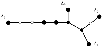
Figure 1. The convex hull of four points in the building $\mathcal{B}_{2}$.

The bases can be determined from the labels of the arrows in Figure 2. A node uses a basis if and only if the node lies on the two-sided infinite path (or apartment) spanned by those arrows. There are eight distinct sets of pairs appearing in the above list, indicating that the tree in Figure 1 is divided into eight cells. This subdivision is the key ingredient in our algorithm. ∎

Returning to our general discussion, we fix an arbitrary finite subset $M=\{f_{1},\ldots,f_{n}\}$ of $K^{d}$ which spans $K^{d}$ as a $K$-vector space, and we consider the set of all equivalence classes of lattices of the form $\,\Lambda\,=\,R\bigl{\{}z^{-u_{1}}f_{1},\,z^{-u_{2}}f_{2},\,z^{-u_{3}}f_{3},\,\ldots,\,z^{-u_{n}}f_{n}\bigr{\}},$ where $u_{1},u_{2},\ldots,u_{n}$ are any integers. This set of lattice classes is called the membrane spanned by $M$ in the Bruhat–Tits building $\,\mathcal{B}_{d}$. We denote the membrane by $\,[M]$, and we identify it with the simplicial complex obtained by restricting $\mathcal{B}_{d}$ to $[M]$. If $n=d$, so that $M$ is a basis of $K^{d}$, then the membrane $[M]$ is known as an apartment of the building $\mathcal{B}_{d}$.

Lemma 4.

(Keel and Tevelev [17, Lemma 4.13])  The membrane $[M]$ is the union of the apartments which can be formed from any $d$ linearly independent columns of $M$.

For instance, if we take $M=\{a,b,c,d,e,f,g,h\}\subset K^{2}$ as in Example 3, then the membrane $[M]$ is an infinite tree with seven unbounded rays, as shown in Figure 2 and derived in Example 19 below. The convex hull of $\Lambda_{1}=R\{a,b\}$, $\Lambda_{2}=R\{c,d\}$, $\Lambda_{3}=R\{e,f\}$ and $\Lambda_{4}=R\{g,h\}$ was constructed as a finite subcomplex of the infinite tree $[M]$.

Figure 2. A one-dimensional membrane is an infinite tree.

The term “membrane” was coined by Keel and Tevelev [17] who showed that $[M]$ is a triangulation of the tropicalization of the subspace of $K^{n}$ spanned by the rows of the $d\times n$-matrix $[f_{1},\ldots,f_{n}]$. This result is implicit in the work of Dress and Terhalle [8, 9]. The precise statement and a self-contained proof will be given in Theorem 18 below.

The membrane $[M]$ is obviously max-convex in $\mathcal{B}_{d}$. However, for $d\geq 3$, membranes are generally not min-convex. Here is a simple example which shows this:

Example 5.

We consider the $3\times 5$-matrix

$$M\,\,=\,\,(f_{1},f_{2},f_{3},f_{4},f_{5})\,\,=\,\,\left(\begin{array}[]{ccccc}z&0&0&1&1\\ 0&1&0&1&0\\ 0&0&1&0&1\end{array}\right)$$

The lattices $\,\Lambda_{1}=R\{f_{1},f_{2},f_{3}\}\,$ and $\,\Lambda_{2}=R\{f_{1},f_{4},f_{5}\}\,$ are in the membrane $[M]$. However, their intersection $\,\Lambda_{1}\cap\Lambda_{2}\,=\,R(0,1,-1)+zR^{3}\,$ is a lattice which is not in $[M]$. ∎

While apartments and membranes are infinite subcomplexes of the Bruhat–Tits building $\mathcal{B}_{d}$, they have a natural finite presentation by matrices whose columns are in $K^{d}$. We can thus ask computational questions about apartments and membranes, such as:

Computational Problem B. Compute the intersection of $s$ given apartments (or membranes) in $\mathcal{B}_{d}$. The input is represented by rank $d$ matrices $M_{1},\ldots,M_{s}$ having $d$ rows with entries in $K$. The $i$-th apartment (or membrane) is spanned by the columns of $M_{i}$. The desired intersection is a locally finite simplicial complex of dimension $\leq d-1$.

General solutions to Problems A and B, based on tropical convexity, will be presented in Sections 5 and 6. At this point, the reader may wish to contemplate our two problems for the special case $d=2$: the intersection of apartments is a path which is usually finite.

Remark 6.

In the theory of buildings there is another frequently used notion of convexity. Following [1, §3.6.2], it rests on the following definitions. The maximal simplices in the Bruhat–Tits building $\mathcal{B}_{d}$ are called chambers. A set $\mathcal{C}$ of chambers is convex if every chamber on a shortest path (in the dual graph of the simplicial complex $\mathcal{B}_{d}$) between two chambers of $\mathcal{C}$ also lies in $\mathcal{C}$. This notion of convexity on $\mathcal{B}_{d}$ agrees with convexity induced by shortest geodesics on spaces of non-positive curvature, and it is related to decompositions of semi-simple Lie groups [14]. Apartments and sub-buildings as well as intersections of convex sets are convex. A set of chambers contained in an apartment is convex if and only if it is the intersection of roots (or half-apartments). In a thick building, such as $\mathcal{B}_{d}$, every root is the intersection of two apartments. Hence any convex set within some apartment of $\mathcal{B}_{d}$ arises as the output of an algorithm for Computational Problem B. Such algorithms are our topic in Section 6. The relationship of this classical convexity in $\mathcal{B}_{d}$ to min- and max-convexity will be clarified in Proposition 20 and Theorem 27.

3. Tropical polytopes

We review the basics of tropical convexity from [7]. A subset $P$ of $\mathbb{R}^{d}$ is called tropically convex if it is closed under linear combinations in the min-plus algebra, i.e. for any two vectors $x=(x_{1},\dots,x_{d})$ and $y=(y_{1},\dots,y_{d})$ in $P$ and any scalars $\lambda,\mu\in\mathbb{R}$ we also have

$$\bigl{(}\min(x_{1}+\lambda,y_{1}+\mu),\ldots,\min(x_{d}+\lambda,y_{d}+\mu)\bigr{)}\,\,\,\in\,\,P.$$

It has become customary to write the tropical arithmetic operations as

$$x\oplus y\ :=\ \min(x,y)\quad\text{and}\quad x\odot y\ :=\ x+y\,.$$

In particular, if $x=(x_{1},\dots,x_{d})\in P$ then $\lambda\odot x:=(\lambda\odot x_{1},\dots,\lambda\odot x_{d})\in P$ for all $\lambda$. Thus we can identify each tropically convex set $P\subset\mathbb{R}^{d}$ with its image in the tropical projective space, which is defined as the quotient space

$$\mathbb{T}\mathbb{P}^{d-1}\quad:=\quad\mathbb{R}^{d}/\mathbb{R}(1,1,\dots,1)\,.$$

There is a natural metric $\delta$ on tropical projective space $\mathbb{T}\mathbb{P}^{d-1}$ which is given as follows:

(2) $$\delta(x,y)\quad:=\quad\max_{1\leq i<j\leq d}|x_{i}+y_{j}-x_{j}-y_{i}|.$$

The following characterizes the projection to the nearest point in a closed convex set.

Proposition 7.

Let $x\in\mathbb{T}\mathbb{P}^{d-1}$ and $P$ a closed tropically convex set in $\mathbb{T}\mathbb{P}^{d-1}$. Among all points $w$ in $P$ that satisfy $\,w\geq x\,$ there is a unique coordinate-wise minimal point. (Here “$w\geq x$” means that there exist representative vectors $w,x\in\mathbb{R}^{d}$ with $w_{i}\geq x_{i}$ for all $i$). This point, which is denoted $\pi_{P}(x)$, minimizes the $\delta$-distance from $x$ to $P$.

Proof.

If $w,w^{\prime}\in P$ then the coordinate-wise minimum $\min(w,w^{\prime})$ also lies in $P$. Since $P$ is closed, it follows that the set $\{w\in P:w\geq x\}$ has a minimal point $y$. We claim that $y$ is $\delta$-closest to $x$ among all points in $P$. Consider any point $y^{\prime}\in P$. After translation we may assume $x=0$ and that both $y$ and $y^{\prime}$ have its smallest coordinate zero. Then $\delta(x,y)$ is the largest coordinate of $y$, and $\delta(x,y^{\prime})$ is the largest coordinate of $y^{\prime}$. By construction of $y=\pi_{P}(x)$, we have $y_{i}\leq y^{\prime}_{i}$ for all $i$, and hence $\delta(x,y)\leq\delta(x,y^{\prime})$. ∎

The map $\pi_{P}\,:\,\mathbb{T}\mathbb{P}^{d-1}\rightarrow P,\,x\mapsto\pi_{P}(x)$ is the nearest point map onto $P$. Clearly, $\pi_{P}(x)=x$ if and only if $x\in P$. We now give an explicit formula for $\pi_{P}$ in the special case when $P$ is a tropical polytope. This means that $P$ is the smallest tropically convex set containing a given finite collection of points $v_{1},v_{2},\dots,v_{n}\in\mathbb{T}\mathbb{P}^{d-1}$. Thus $P$ is the tropical convex hull of these points, in symbols, $P=\operatorname{tconv}(v_{1},v_{2},\ldots,v_{n})$.

Lemma 8.

The $i$-th coordinate of the nearest point map onto the tropical polytope $P=\operatorname{tconv}(v_{1},v_{2},\ldots,v_{n})$ in $\mathbb{T}\mathbb{P}^{d-1}$ is given by the formula

$$\pi_{P}(x)_{i}\,\,=\,\,\min_{k\in\{1,\ldots,n\}}\max_{j\in\{1,\ldots,d\}}(v_{ki}-v_{kj}+x_{j}).$$

Proof.

Set $y_{i}=\min_{k=1}^{n}\max_{j=1}^{d}(v_{ki}-v_{kj}+x_{j})$. Taking $j=i$ in the maximum, we see that the vector $y=(y_{1},\dots,y_{d})$ satisfies $y\geq x$. Writing $y_{i}=\min_{k=1}^{n}(\max_{j=1}^{d}(x_{j}\!-\!v_{kj})+v_{ki})$, we find that $y$ is a tropical linear combination of the points $v_{1},\dots,v_{n}$. Hence $y$ lies in $P$. Moreover, $y$ is the coordinate-wise minimal vector in $\mathbb{R}^{d}$ with these two properties. ∎

Example 9.

There may be several points in a tropical polytope $P$ which minimize the distance to a given point $x$. Consider the point $x=(0,1,1)$ in the plane $\mathbb{T}\mathbb{P}^{2}$ and the one-dimensional polytope $P=\operatorname{tconv}((1,0,0),(0,1,0),(0,0,1))$. The projection of $x$ onto $P$ is $\pi_{P}(x)=(0,0,0)=(1,1,1)$, but $\,\delta(x,(0,0,0))\,=\,\delta(x,(0,0,1))\,=\,\delta(x,(0,1,0))\,=\,1$. ∎

The formula in Lemma 8 specifies a subdivision of the tropical polytope $P$ into cells. These cells are ordinary polytopes of the special form

(3) $$\quad\left\{\,w\in\mathbb{T}\mathbb{P}^{d-1}\vphantom{w_{i}-w_{j}\leq u_{ij}\text{ for all $i\neq j$ }}\,:\,\vphantom{w\in\mathbb{T}\mathbb{P}^{d-1}}w_{i}-w_{j}\leq u_{ij}\text{ for all $i\neq j$ }\,\right\}\qquad(\text{for some }u_{ij}\in\mathbb{R}).\!\!\!$$

The cell containing $x\in P$ is specified by its type, which is the collection of index sets where “$\min$” and “$\max$” are attained in the identity $\pi_{P}(x)=x$. To be precise, we define $\operatorname{type}(x):=(S_{1},S_{2},\ldots,S_{d})$, where

(4) $$\begin{split}S_{i}\ &=\ \left\{\,k\in\{1,\ldots,n\}\vphantom{\max_{j\in\{1,\dots,d\}}(v_{ki}-v_{kj}+x_{j})\,=\,x_{i}}\,:\,\vphantom{k\in\{1,\ldots,n\}}\max_{j\in\{1,\dots,d\}}(v_{ki}-v_{kj}+x_{j})\,=\,x_{i}\,\right\}\\ &=\ \left\{\,k\vphantom{v_{ki}-x_{i}\,=\,\min(v_{k1}-x_{1},v_{k2}-x_{2},\ldots,v_{kd}-x_{d})}\,:\,\vphantom{k}v_{ki}-x_{i}\,=\,\min(v_{k1}-x_{1},v_{k2}-x_{2},\ldots,v_{kd}-x_{d})\,\right\}\,.\end{split}$$

Two points of $P$ lie in the same cell if and only if they have the same type. This subdivision of $P$ depends on the chosen generators $v_{1},v_{2},\ldots,v_{n}$ and not just on the set $P$.

Remark 10.

The sets $\,\left\{\,w\in\mathbb{T}\mathbb{P}^{d-1}\vphantom{w_{i}-w_{j}\,\leq\,u}\,:\,\vphantom{w\in\mathbb{T}\mathbb{P}^{d-1}}w_{i}-w_{j}\,\leq\,u\,\right\}\,$ are the ordinary affine halfspaces which are also tropically convex. For integral $u$ we call such a halfspace a root of $\mathbb{T}\mathbb{P}^{d-1}$.

A point in the tropical projective space $\mathbb{T}\mathbb{P}^{d-1}$ is a lattice point if it is represented by a vector $x$ in $\mathbb{Z}^{d}$. We define a graph on the set of all lattice points as follows: two points $x$ and $y$ are connected by an edge if and only if $\delta(x,y)=1$. The $\delta$-distance between any two lattice points in $\mathbb{T}\mathbb{P}^{d-1}$ is the shortest length of any path connecting these two points in the graph. A tropical lattice polytope is the tropical convex hull of finitely many lattice points in $\mathbb{T}\mathbb{P}^{d-1}$. The cells of a tropical lattice polytope are intersections of roots.

Theorem 11.

The flag simplicial complex defined by this graph is a triangulation of the affine space $\mathbb{T}\mathbb{P}^{d-1}$. It restricts to a triangulation of each cell (3) of each tropical lattice polytope $P$. We refer to this as the standard triangulation of $\mathbb{T}\mathbb{P}^{d-1}$, or of $P$, or of (3).

Proof.

We represent points in $\mathbb{T}\mathbb{P}^{d-1}$ by vectors with first coordinate zero. This identifies the lattice points in $\mathbb{T}\mathbb{P}^{d-1}$ with $\mathbb{Z}^{d-1}$. The maximal simplices in the flag complex are

$$\bigl{\{}a,a+e_{\sigma_{2}},a+e_{\sigma_{2}}+e_{\sigma_{3}},\dots,a+e_{\sigma_{2}}+e_{\sigma_{3}}+\dots+e_{\sigma_{d}}\bigr{\}}\,,$$

where $u\in\mathbb{Z}^{d-1}$ and $\sigma$ is any permutation of $\{2,\dots,d\}$. If we fix $a$ and let $\sigma$ range over all $(d-1)!$ permutations then these simplices triangulate the unit cube with lower vertex $a$. Putting all these triangulated cubes together, we see that the flag complex is a triangulation of $\mathbb{T}\mathbb{P}^{d-1}$. Each simplex in this standard triangulation is the solution set to a system of inequalities $w_{i}-w_{j}\leq u_{ij}$ where $u_{ij}+u_{ji}\leq 1$ for all $1\leq i<j\leq d$. This implies that if $w$ is any point in a cell (3) then that cell contains the entire simplex of the standard triangulation which has $w$ in its relative interior. Therefore the standard triangulation of $\mathbb{T}\mathbb{P}^{d-1}$ induces a triangulation of every tropical lattice polytope. ∎

Figure 3. The tropical convex hull of nine labeled lattice points in $\mathbb{T}\mathbb{P}^{2}$. Dashed lines and white points indicate the standard triangulation of this polygon. Solid lines and black points show the decomposition into cells (3).

Example 12 ($d=3,n=9$).

Let $v_{1},v_{2},\ldots,v_{9}$ denote the columns of

(5) $$V\,\,\,=\,\,\,\begin{pmatrix}\phantom{-}0&\phantom{-}0&\phantom{-}0&1&-3&1&-3&-4&0\,\\ -5&-4&-8&0&\phantom{-}0&0&-7&-8&0\,\\ -3&\phantom{-}2&-3&0&-2&2&\phantom{-}0&\phantom{-}0&0\,\end{pmatrix}$$

We compute the tropical convex hull $\,P=\operatorname{tconv}(v_{1},\ldots,v_{9})\,$ in $\mathbb{T}\mathbb{P}^{2}$. The tropical lattice polygon $P$ has ten $2$-dimensional cells, $28$ edges, and $19$ vertices. Hence there are $10+28+19=57$ distinct types $\,\operatorname{type}(x)=(S_{1},S_{2},S_{3})\,$ among the points $x$ in $P$. The standard triangulation of $P$ is a simplicial complex with $32$ triangles, $62$ edges and $31$ vertices, namely, the lattice points in $P$. It is depicted in Figure 3. ∎

By [7, Theorem 23], the convex hull of the rows of a matrix equals the convex hull of the columns of that same matrix. Indeed, if $V$ is the $d\times n$-matrix whose columns are the vectors $v_{i}$ then the cell complex on $P=\operatorname{tconv}(v_{1},\ldots,v_{n})$ defined by the types is isomorphic to the cell complex on the convex hull in $\mathbb{T}\mathbb{P}^{n-1}$ of the $d$ row vectors of $V$.

Example 13.

(Self-Duality of Tropical Polytopes)  Let $v^{\prime}_{1},v^{\prime}_{2},v^{\prime}_{3}$ be the row vectors of the matrix $V$ in (5), and let $P^{\prime}=\operatorname{tconv}(v^{\prime}_{1},v^{\prime}_{2},v^{\prime}_{3})$ be their tropical convex hull in $\mathbb{T}\mathbb{P}^{8}$. The tropical triangle $P^{\prime}$ contains precisely the following $31$ lattice points:

${\bf(\underline{\bf 4},\underline{\bf 4},\underline{\bf 4},5,1,5,1,0,4)}$	$(\underline{4},\underline{4},\underline{3},5,1,5,1,0,4)$	$(\underline{4},\underline{4},\underline{2},5,1,5,1,0,4)$
$(\underline{4},\underline{4},\underline{1},5,1,5,1,0,4)$	$(\underline{3},\underline{4},\underline{3},5,1,5,1,0,4)$	$(\underline{3},\underline{4},\underline{2},5,1,5,1,0,4)$
$(\underline{3},\underline{4},\underline{1},5,1,5,1,0,4)$	$(\underline{3},\underline{4},\underline{0},5,1,5,1,0,4)$	$(\underline{2},\underline{4},\underline{2},5,1,5,1,0,4)$
$(\underline{2},\underline{4},\underline{1},5,1,5,1,0,4)$	$(\underline{2},\underline{4},\underline{0},5,1,5,1,0,4)$	$(\underline{3},\underline{4},0,\underline{6},2,6,1,0,5)$
$(\underline{3},4,0,\underline{7},\underline{3},7,1,0,6)$	$(\underline{3},4,0,\underline{8},\underline{4},8,1,0,7)$	$(\underline{1},\underline{4},\underline{1},4,1,5,1,0,4)$
$(\underline{1},\underline{4},\underline{0},4,1,5,1,0,4)$	$(\underline{2},\underline{4},0,5,\underline{2},6,1,0,5)$	$(\underline{3},\underline{4},0,6,\underline{3},7,1,0,6)$
$(\underline{3},4,0,\underline{7},\underline{4},8,1,0,7)$	$(\underline{3},4,0,\underline{8},\underline{5},8,1,0,8)$	$(\underline{0},\underline{4},\underline{0},3,1,5,1,0,3)$
$(\underline{1},\underline{4},0,4,\underline{2},6,1,0,4)$	$(\underline{2},\underline{4},0,5,\underline{3},7,1,0,5)$	$(\underline{3},\underline{4},0,6,\underline{4},8,1,0,6)$
$(\underline{3},4,0,\underline{7},\underline{5},8,1,0,7)$	$(\underline{3},4,0,\underline{8},\underline{6},8,1,0,8)$	$(\underline{3},4,0,\underline{8},\underline{7},8,1,0,8)$
${\bf(\underline{\bf 3},4,0,\underline{\bf 8},\underline{\bf 8},8,1,0,8)}$	$(\underline{0},\underline{5},\underline{0},3,1,5,2,1,3)$	$(\underline{0},5,\underline{0},3,1,5,\underline{3},2,3)$
${\bf(\underline{\bf 0},5,\underline{\bf 0},3,1,5,3,\underline{\bf 3},3)}$

Here each point is represented uniquely by a non-negative vector with a zero entry. The boldfaced vectors represent the given points $v^{\prime}_{1},v^{\prime}_{2},v^{\prime}_{3}\in\mathbb{T}\mathbb{P}^{8}$. The underlined triples of coordinates will be explained in Example 23. The tropical triangle $P^{\prime}$, which lives in $\mathbb{T}\mathbb{P}^{8}$, is isomorphic to the tropical $9$-gon $P$ of Example 12, which lives in $\mathbb{T}\mathbb{P}^{2}$ and is depicted in Figure 3. According to equation (14) in [7, page 16], the isomorphism between the two tropical polygons is given by the piecewise-linear maps

(6) $$\begin{split}P\rightarrow P^{\prime},\ &(x_{1},x_{2},x_{3})\,\mapsto\bigl{(}\min_{i=1}^{3}(v_{i1}-x_{i}),\ldots,\min_{i=1}^{3}(v_{i9}-x_{i})\bigr{)}\,,\\ P^{\prime}\rightarrow P,\ &(y_{1},\ldots,y_{9})\mapsto\bigl{(}\min_{j}(v_{1j}{-}y_{j}),\dots,\min_{j}(v_{3j}{-}y_{j})\bigr{)}\,.\end{split}$$

These bijections are inverses of each other. They are linear on each cell, and they identify the types: if $x\in P$ and $\operatorname{type}(x)=(S_{1},S_{2},S_{3})$ then the corresponding point $y\in P^{\prime}$ has $\operatorname{type}(y)=(S^{\prime}_{1},S^{\prime}_{2},\ldots,S^{\prime}_{9})$ where $\,S^{\prime}_{j}=\{i:j\in S_{i}\}$. The $31$ lattice points in $\mathbb{T}\mathbb{P}^{8}$ that are listed above get sent to the $31$ lattice points in Figure 3 by the map $P^{\prime}\rightarrow P$. ∎

We close with the remark that several algorithms are available for computing a tropical polytope $P$ from its defining matrix $V=(v_{ij})$. They will be discussed in Section 5.

4. Tropical linear spaces and membranes

This section is concerned with the relationship between tropical linear spaces, valuated matroids [8, 9], and membranes [17] in the Bruhat–Tits building. In order to think of these objects as tropical polytopes, we shall now augment the real numbers $\mathbb{R}$ by the extra element $\infty$. Note that $\infty$ is the additively neutral element in the min-plus algebra. We define the compactified tropical projective space $\overline{\mathbb{T}\mathbb{P}}^{d-1}$ to be $(\mathbb{R}\cup\{\infty\})^{d}\setminus\{(\infty,\ldots,\infty)\}$ modulo the equivalence relation given by tropical scalar multiplication. The notions of tropical convexity, tropical polytopes and lattice points make sense in $\overline{\mathbb{T}\mathbb{P}}^{d-1}$. When extending the metric $\delta$ to $\overline{\mathbb{T}\mathbb{P}}^{d-1}$ we use the convention that $\infty-\infty=0$ in the formula (2). Proposition 7 and Lemma 8 remain valid, and there is a standard triangulation of $\overline{\mathbb{T}\mathbb{P}}^{d-1}$. That standard triangulation coincides with the compactified apartment in the work of Werner [25, 26]. We also refer to Alessandrini [2] whose tropical approach to buildings is similar to ours and is aimed at applications in Teichmüller theory.

For experts on buildings we note that our two notions of convexity in Problem A reflect two different compactifications of the Bruhat–Tits buildings $\mathcal{B}_{d}$. The first is featured in [18, 25] and we call it the max-compactification. It is a simplicial complex whose vertices are all free $R$-submodules of $K^{d}$, and the boundary consists of modules of rank less than $d$. The second compactification, which we call the min-compactification, arises more naturally from tropical geometry. Its points consist of all additive seminorms on $K^{d}$. An additive seminorm is a function $N:K^{d}\rightarrow\mathbb{R}\cup\{\infty\}$ which satisfies the first two axioms of an additive norm. If $N$ is an additive seminorm then $N^{-1}(\infty)$ is a linear subspace of $K^{d}$. The boundary of the min-compactification consists of additive seminorms for which $N^{-1}(\infty)$ is positive-dimensional. We shall not dwell on the matters here, but we do wish to underline that our combinatorial results are compatible with these compactifications.

We now review the definition of tropical linear spaces [22, 23]. Fix two positive integers $d\leq n$ and consider a map $p:\{1,2,\dots,n\}^{d}\rightarrow\mathbb{R}\cup\{\infty\}$. Following Dress and Terhalle [8, 9], we say that $p$ is a valuated matroid if $p(\omega)$ depends only on the unordered set $\{\omega_{1},\dots,\omega_{d}\}$, and $p(\omega)=\infty$ whenever $\omega$ has fewer than $d$ elements, and $p$ satisfies the following variant of the basis exchange axiom: for any $(d-1)$-subset $\sigma$ and any $(d+1)$-subset $\tau$ of $\{1,2,\dots,n\}$, the minimum of the list of numbers $\bigl{(}p(\sigma\cup\tau_{i})+p(\tau\setminus\{\tau_{i}\})\,:\,i=1,2,\ldots,d+1\,\bigr{)}$ is attained at least twice. This axiom is equivalent to saying that $p$ lies in the tropical prevariety [20] specified by the set of all quadratic Plücker relations.

Fix a valuated matroid $p$. The associated tropical linear space $L_{p}$ consists of all points $x\in\overline{\mathbb{T}\mathbb{P}}^{n-1}$ such that, for any $(d{+}1)$-subset $\tau$ of $\{1,2,\dots,n\}$, the minimum of the numbers $\,p(\tau\backslash\{\tau_{i}\})+x_{\tau_{i}}$, for $i=1,2,\ldots,d$, is attained at least twice. This list of numbers represents a circuit of $p$. The tropical linear space $L_{p}$ is tropically convex, and it can be represented as a tropical lattice polytope as follows. For any $(d{-}1)$-subset $\sigma$ of $\{1,\ldots,n\}$ let $p(\sigma*)$ denote the vector in $(\mathbb{R}\cup\{\infty\})^{n}$ whose $j$-th coordinate equals $\,p(\sigma\cup\{j\})$. We regard $p(\sigma*)$ as a point in $\overline{\mathbb{T}\mathbb{P}}^{n-1}$, or, combinatorially, as a cocircuit of the valuated matroid $p$.

Theorem 14.

(Yu and Yuster [27, Theorem 16])   The tropical linear space $L_{p}$ is the tropical convex hull in the compactified tropical projective space $\overline{\mathbb{T}\mathbb{P}}^{n-1}$ of all the cocircuits $\,p(\sigma*)$ of the underlying valuated matroid $p:\{1,2,\dots,n\}^{d}\rightarrow\mathbb{R}\cup\{\infty\}$.

The tropical linear space $L_{p}$ is tropically convex. Hence it has a nearest point map $\pi_{L_{p}}$ which takes any point $x\in\overline{\mathbb{T}\mathbb{P}}^{n-1}$ to the coordinate-wise minimum in $\{w\in L_{p}:w\geq x\}$. We now present two rules for evaluating this map.

The Blue Rule. Form the vector $w\in\mathbb{R}^{n}$ whose coordinates are

(7) $$w_{i}\quad=\quad\min_{\sigma}\,\max_{j\not\in\sigma}\bigl{(}p(\sigma\cup\{i\})-p(\sigma\cup\{j\})+x_{j}\bigr{)}.$$

Here the minimum is over all $(d-1)$-subsets $\sigma$ of $\{1,2,\dots,n\}$.

The Red Rule. Start with $v=(0,0,\ldots,0)$. For any $(d+1)$-set $\tau$ do: If the minimum of the numbers $p(\tau\backslash\{\tau_{i}\})+x_{\tau_{i}}$ is attained only once, for the index $i$, then let $\gamma_{\tau,i}$ be the difference of the second smallest number minus that minimum, and set $v_{\tau_{i}}:=\max(v_{\tau_{i}},\gamma_{\tau,i})$.

The terms Blue Rule and Red Rule were introduced by Ardila [3]. The following theorem extends his main result in [3] from ordinary matroids to valuated matroids:

Theorem 15.

Let $p$ be a valuated matroid, $L_{p}$ its tropical linear space and $x\in\overline{\mathbb{T}\mathbb{P}}^{n-1}$. If $v$ and $w$ are computed by the Red Rule and the Blue Rule then $\pi_{L_{p}}(x)\,=\,x+v\,=\,w$.

Sketch of Proof.

In the case of ordinary matroids, the image of $p$ lies in $\{0,\infty\}$. This special case is [3, Theorem 1]. Ardila’s proof easily generalizes to valuated matroids. The correctness of the Blue Rule also follows from Lemma 8 and Theorem 14. ∎

Remark 16.

The Red Rule and the Blue Rule produce the identical result in the special case when $x=(0,0,\ldots,0)$. We find that $\,\pi_{P}(0,0,\dots,0)\in L_{p}\,$ is the tropical sum of all cocircuits $p(\sigma*)$ of the valuated matroid $p$, provided each cocircuit is represented by the unique vector whose coordinates are non-negative and has at least one coordinate zero.

We now apply tropical convexity to the Bruhat–Tits building $\mathcal{B}_{d}$. We begin with a review on how tropical linear spaces are related to ordinary linear spaces over the field $K=\mathbb{C}(\!(x)\!)$. Let $M$ be a $d\times n$-matrix of rank $d$ with entries in $K$. The row space of $M$ is a $d$-dimensional linear subspace of $K^{n}$, or a $(d-1)$-dimensional subspace of the projective space $\mathbb{P}^{n-1}_{K}$. If $\omega$ is an ordered list of $d$ elements in $\{1,2,\dots,n\}$ then $M_{\omega}$ denotes the corresponding $d\times d$-submatrix. The matrix $M$ defines a valuated matroid $p$ by the rule

(8) $$p(\omega)\quad=\quad\operatorname{val}\bigl{(}\det(M_{\omega})\bigr{)}\,.$$

Note that $p(\omega)=\infty$ if and only if $M_{\omega}$ is not invertible over $K$.

Proposition 17.

(Speyer and Sturmfels [23, Theorem 2.1]) The lattice points in the tropical linear space $L_{p}$ are precisely the points $\operatorname{val}(v)$ where $v$ is in the row space of $M$.

Since $L_{p}$ is a tropical lattice polytope, the standard triangulation of $\overline{\mathbb{T}\mathbb{P}}^{n-1}$ restricts to a triangulation of $L_{p}$. We shall present a self-contained proof of the following result.

Theorem 18.

(Keel and Tevelev [17, Theorem 4.15]) Let $\,M=(f_{1},f_{2},\ldots,f_{n})\,$ be a $d\times n$-matrix of rank $d$ over $K$, and let $L_{p}$ be the associated tropical linear space. Then

$$\Psi_{M}\,:\,R\bigl{\{}z^{-u_{1}}f_{1},\,z^{-u_{2}}f_{2},\,\ldots,\,z^{-u_{n}}f_{n}\bigr{\}}\,\mapsto\,\pi_{L_{p}}(u_{1},u_{2},\dots,u_{n})$$

is a well-defined map, and it induces an isomorphism of simplicial complexes between the membrane $[M]$ and the standard triangulation of $L_{p}$.

Proof.

Consider any lattice $\,\Lambda=R\bigl{\{}z^{-u_{1}}f_{1},\,z^{-u_{2}}f_{2},\,\ldots,\,z^{-u_{n}}f_{n}\bigr{\}}\,$ in the membrane, and set $(v_{1},v_{2},\ldots,v_{n})=\pi_{L_{p}}(u_{1},u_{2},\ldots,u_{n})$. We claim that

(9) $$v_{i}\quad=\quad\max\{\,\mu\in\mathbb{Z}\,:\,z^{-\mu}f_{i}\in\Lambda\,\}.$$

We first prove the inequality “$\leq$”. By the Red Rule in Theorem 15, we have $v_{i}=\gamma_{\tau,i}+u_{i}$ for some $(d+1)$-set $\tau$ containing $i$. We may assume $\tau_{d+1}=i$. Then $\{f_{\tau_{1}},\dots,f_{\tau_{d}}\}$ is a basis of $K^{d}$, and we can write

$$\quad f_{i}\quad=\quad p_{1}f_{\tau_{1}}+p_{2}f_{\tau_{2}}+\cdots+p_{d}f_{\tau_{d}}\qquad\quad\hbox{for some}\,\,p_{1},\ldots,p_{d}\in K.$$

Our choice of the $(d+1)$-set $\tau$ in the Red Rule means that

$$u_{i}+\gamma_{\tau,i}\quad=\quad\min\{\,\operatorname{val}(p_{j})+u_{\tau_{j}}\,:\,j=1,2,\dots,d\,\}\quad\geq\quad 0\,,$$

and therefore

(10) $$f_{i}z^{-u_{i}-\gamma_{\tau,i}}\,\,\,=\,\,\,p_{1}z^{u_{\tau_{1}}}(f_{\tau_{1}}z^{-u_{\tau_{1}}})+\cdots+p_{d}z^{u_{\tau_{d}}}(f_{\tau_{d}}z^{-u_{\tau_{d}}})\,\,\in\,\,\Lambda\,.$$

This proves the inequality “$\leq$”. The converse “$\geq$” holds because $z^{-\mu}f_{i}$ lies in $\Lambda$ if and only it lies in the $R$-submodule spanned by $d$ of the $n$ generators, and a representation (10) is the only way this can happen. Indeed, by Lemma 4, the membrane $[M]$ is the union of the apartments $[(f_{\tau_{1}},\dots,f_{\tau_{d}})]$ for all $d$-subsets $\tau\subseteq\{1,2,\dots,n\}$.

The identity (9) shows that the map $\Psi_{M}$ which takes the lattice $R\bigl{\{}z^{-u_{1}}f_{1},\dots,\,z^{-u_{n}}f_{n}\bigr{\}}$ to the point $\pi_{L_{p}}(u_{1},\dots,u_{n})$ is well-defined, and is a bijection between the membrane $[M]$ and the lattice points in the tropical linear space $L_{p}$. This bijection takes adjacent lattices to points of $\delta$-distance one in $L_{p}$ and conversely. Hence it induces an isomorphism between the flag simplicial complexes of these two graphs. ∎

Example 19.

Let $d=2$, $n=8$ and let $\,M=(a,b,c,d,e,f,g,h)\,$ be as in Example 3. The valuated matroid $\,p\,$ of the matrix $\,M\,$ maps pairs of columns to $\mathbb{Z}\cup\{\infty\}$ as follows:

$$\begin{pmatrix}aa&\!ab&\!ac&\cdots&ah\\ ab&\!bb&\!bc&\cdots&bh\\ ac&\!bc&\!cc&\cdots&ch\\ \vdots&\vdots&\vdots&\ddots&\vdots\\ ah&\!bh&\!ch&\cdots&hh\end{pmatrix}\mapsto\begin{pmatrix}\infty&-7&-2&\infty&-1&-7&-3&-2\\ -7&\infty&-3&-5&-1&-8&-4&-3\\ -2&-3&\infty&0&3&-1&2&4\\ \infty&-5&0&\infty&1&-5&-1&0\\ -1&-1&3&1&\infty&-2&2&3\\ -7&-8&-1&-5&-2&\infty&-3&0\\ -3&-4&2&-1&2&-3&\infty&2\\ -2&-3&4&0&3&0&2&\infty\end{pmatrix}$$

The rows of this $8{\times}8$-matrix are the cocircuits $p(\sigma*)$ of the valuated matroid $p$. They represent seven distinct points in $\overline{\mathbb{T}\mathbb{P}}^{7}\,$ (rows $1$ and $4$ give the same point). The tropical linear space $L_{p}$ is the tropical convex hull of these seven points in $\overline{\mathbb{T}\mathbb{P}}^{7}$. This convex hull is the tree depicted in Figure 2. A systematic algorithm for drawing such a tree $L_{p}$, given its valuated matroid $p$, is the neighbor-joining method from phylogenetics; see [23, §6]. ∎

Theorem 18 states that every lattice point $(u_{1},\ldots,u_{n})$ in $L_{p}$ uniquely represents a lattice $\Lambda_{u}=R\bigl{\{}z^{-u_{1}}f_{1},\,\ldots,\,z^{-u_{n}}f_{n}\bigr{\}}$ in the membrane $[M]$. The lattice $\Lambda_{u}$ specifies a matroid $M_{u}$ of rank $d$ on $\{1,2,\ldots,n\}$. This is an ordinary (not valuated) matroid. The bases of $M_{u}$ are the sets $\{\tau_{1},\ldots,\tau_{d}\}$ such that $\,\{z^{-u_{\tau_{1}}}f_{\tau_{1}},\,\ldots,\,z^{-u_{\tau_{d}}}f_{\tau_{d}}\}\,$ spans the lattice $\Lambda$. The matroid $M_{u}$ can be read off directly from the valuated matroid $p$ as follows: its bases are the $d$-sets $\tau$ such that the expression $\,p(\tau)-u_{\tau_{1}}-\cdots-u_{\tau_{d}}\,$ is minimal. The set of all matroids $M_{u}$, as $u$ ranges over the tropical linear space $L_{p}$, forms a matroid subdivision of the matroid polytope of the matrix $M$ over the field $K$. This is the identification of tropical linear spaces with matroid subdivisions as studied in [16, 22].

Our algorithm for Computational Problem A in Section 5 will output each lattice $\Lambda_{u}$ in the min-convex hull as a pair $(u,M_{u})$, where $u$ is a point in a tropical linear space $L_{p}$ and $M_{u}$ is a matroid. We saw this format already in Example 3. For instance, consider the point $u=(2,0,5,4,6,0,4,5)$ listed there. It lies the tropical line $L_{p}$ of Example 19. The rank $2$ matroid $M_{u}$ has the set of bases $\{ab,ac,ae,af,ag,ah,bd,cd,de,df,dg,dh\}$.

The classical notion of convexity in buildings in Remark 6 is related to tropical convexity as follows. For a chamber $C$ in $\mathcal{B}_{d}$ let $\operatorname{vert}(C)$ be its set of vertices. Now consider a set $\mathcal{C}$ of chambers contained in some apartment $\mathcal{A}$. We identify $\mathcal{A}$ with $\mathbb{T}\mathbb{P}^{d-1}$ and we note that the classical notion of a root (or half-apartment) of $\mathcal{A}$ agrees with our definition of a root in $\mathbb{T}\mathbb{P}^{d-1}$ from Remark 10. We consider the following set of lattice points in $\mathbb{T}\mathbb{P}^{d-1}$:

$$\operatorname{vert}(\mathcal{C})\ :=\ \bigcup\left\{\,\operatorname{vert}(C)\vphantom{C\in\mathcal{C}}\,:\,\vphantom{\operatorname{vert}(C)}C\in\mathcal{C}\,\right\}$$

Our next result holds because the convex subsets of chambers in $\mathcal{A}$ are intersections of roots, or equivalently, intersections of $\mathcal{A}$ with other apartments. See also Theorem 27.

Proposition 20.

A finite set $\mathcal{C}$ of chambers in an apartment $\mathcal{A}\cong\mathbb{T}\mathbb{P}^{d-1}$ is convex if and only if $\operatorname{vert}(\mathcal{C})$ is the set of lattice points in a tropical lattice polytope of the form (3).

Proposition 20 implies that the convex sets of chambers are precisely the maximal simplices in the standard triangulation of those tropical lattice polytopes which are at the same time (possibly unbounded) ordinary convex polyhedra. In other words, Proposition 20 holds verbatim for infinite $\,\mathcal{C}\,$ if $\,\mathbb{T}\mathbb{P}^{d-1}\,$ is replaced by its compactification $\,\overline{\mathbb{T}\mathbb{P}}^{d-1}$.

5. Convex hulls in the Bruhat–Tits building

In this section and the next we present algorithmic implications of the theory developed so far. We begin with Computational Problem A: how to find min-convex hulls in $\mathcal{B}_{d}$. The input is a list of $s$ invertible $d\times d$-matrices $M_{1},M_{2},\dots,M_{s}$ with entries in the field $K=\mathbb{C}(\!(z)\!)$, each representing the equivalence class of its column lattice $\Lambda_{i}=\operatorname{image}_{R}(M_{i})$.

5.1. The retraction of min-convex hulls to a membrane

Let $M=(f_{1},\dots,f_{n})$ be any matrix in $K^{d\times n}$ of rank $d$ and let $[M]$ be the membrane in $\mathcal{B}_{d}$ which is spanned by the $n$ column vectors of $M$. There is a natural retraction $r_{M}$ from $\mathcal{B}_{d}$ onto $[M]$ given by

(11) $$r_{M}:\Lambda\mapsto(\Lambda\cap K\{f_{1}\})+\cdots+(\Lambda\cap K\{f_{n}\})$$

This map restricts to the identity on the membrane $[M]$.

Let $V$ be the $d$-dimensional subspace of $K^{n}$ spanned by the rows of $M$, and let $p$ be its valuated matroid as in formula (8). By Proposition 17, the tropicalization of the classical linear space $V$ over the field $K$ equals the tropical linear space $L_{p}$. The map $\Psi_{M}$ in Theorem 18 allows us to identify the lattice points in $L_{p}$ with the membrane $[M]$.

Lemma 21.

Fix a membrane $[M]$ in $\mathcal{B}_{d}$ and consider any lattice $\Lambda=\operatorname{image}_{R}(M_{0})$ where $M_{0}\in GL_{K}(d)$. Then the following three lattice points in $\overline{\mathbb{T}\mathbb{P}}^{n-1}$ coincide:

1. $\Psi_{M}(r_{M}(\Lambda))$, where $\Psi_{M}$ is the bijection of Theorem 18 between $[M]$ and the lattice points in $L_{p}$,

2. $(N_{\Lambda}(f_{1}),\dots,N_{\Lambda}(f_{n}))$, where $N_{\Lambda}$ is the integral additive norm corresponding to $\Lambda$,

3. the tropical sum (coordinatewise minimum) of the rows of the matrix $\,\operatorname{val}(M_{0}^{-1}\cdot M)$.

Proof.

The equivalence of (a) and (b) follow from the definitions of $N_{\Lambda}$ and $r_{M}$, and from equation (9). The equivalence of (b) and (c) follows from equation (1). ∎

As a consequence, we get the following explicit description of the retraction of a min-convex hull onto a membrane. This establishes the correctness of Algorithm 1 below.

Proposition 22.

Let $\Lambda_{1},\Lambda_{2},\ldots,\Lambda_{s}$ be the lattices spanned by the columns of the matrices $M_{1},M_{2},\dots,M_{s}\in GL_{d}(K)$. Let $[M]$ be any membrane in $\mathcal{B}_{d}$. The simplicial complex

$$r_{M}(\operatorname{minconv}(\Lambda_{1},\Lambda_{2},\ldots,\Lambda_{s}))\subset[M]\,$$

coincides with the standard triangulation of the tropical polytope

$$\operatorname{tconv}\bigl{(}\Psi_{M}(r_{M}(\Lambda_{1})),\Psi_{M}(r_{M}(\Lambda_{2})),\dots,\Psi_{M}(r_{M}(\Lambda_{s}))\bigr{)}\,\,\,\subset\,\,L_{p}\,=\,\operatorname{val}(\operatorname{kernel}(M)).$$

Proof.

By the definition of the integral additive norm $N_{\Lambda}$ in formula (1), we have

$$N_{(z^{-a}\Lambda)\cap(z^{-a^{\prime}}\Lambda^{\prime})}\,\,=\,\,\min\left(a+N_{\Lambda},a^{\prime}+N_{\Lambda^{\prime}}\right).$$

By Lemma 21, for any integers $a_{1},a_{2},\dots,a_{s}$, the image under the map $\Psi_{M}$ of the retraction $\,r_{M}(z^{-a_{1}}\Lambda_{1}\cap\cdots\cap z^{-a_{s}}\Lambda_{s})\,$ coincides with the tropical linear combination

$$(a_{1}\odot\Psi_{M}(r_{M}(\Lambda_{1})))\oplus\dots\oplus(a_{s}\odot\Psi_{M}(r_{M}(\Lambda_{s}))).$$

The simplicial complex structure of $[M]$ coincides with the standard triangulation of the tropical linear space $L_{p}$, which induces the simplicial complex structure on the lattice points in the tropical polytope. Hence the retraction of the min-convex hull onto the membrane coincides with the standard triangulation of the tropical polytope. ∎

Input: matrices $M_{1},\ldots,M_{s}\in\operatorname{GL}_{d}(K)$ and a $d\times n$ matrix $M$ over $K$ with rank $d$

Output: retraction $r_{M}(\operatorname{minconv}(\Lambda_{1},\dots,\Lambda_{s}))$ onto the membrane $[M]$, where $\Lambda_{i}=\operatorname{image}_{R}(M_{i})$ for $i=1,\ldots,s$.

for $i\leftarrow 1,2,\dots,s$ do  $\Psi_{M}(r_{M}(\Lambda_{i}))\leftarrow$ tropical sum of the rows of $\operatorname{val}(M_{i}^{-1}\cdot M)$

  return $\,\,\operatorname{tconv}(\Psi_{M}(r_{M}(\Lambda_{1})),\Psi_{M}(r_{M}(\Lambda_{2})),\dots,\Psi_{M}(r_{M}(\Lambda_{s})))$

Algorithm 1 Retraction of a min-convex hull in $\mathcal{B}_{d}$ onto a given membrane.

Example 23.

(Illustration of Algorithm 1)   We consider the three lattices $\Lambda_{1},\Lambda_{2},\Lambda_{3}$ in the Bruhat–Tits building $\mathcal{B}_{3}$ which are represented by the invertible $3\times 3$-matrices

$$M_{1}\,=\,\begin{pmatrix}1&z^{5}&z^{-3}\\ z^{4}&z&z^{-3}\\ z^{-3}&z^{2}&z^{-3}\end{pmatrix},\;M_{2}\,=\,\begin{pmatrix}z^{2}&z^{-2}&z^{2}\\ z^{3}&z^{5}&z^{5}\\ 1&1&z^{4}\end{pmatrix},\;M_{3}\,=\,\begin{pmatrix}z^{2}&z^{-1}&z\\ z^{-2}&z^{-3}&z^{3}\\ z^{3}&z&1\end{pmatrix}.$$

Set $M:=(M_{1},M_{2},M_{3})$. Then the vectors $\Psi_{M}(r_{M}(\Lambda_{1}))$, $\Psi_{M}(r_{M}(\Lambda_{2}))$, and $\Psi_{M}(r_{M}(\Lambda_{3}))$ are the precisely the rows of the $3\times 9$-matrix $V$ in (5). That matrix was analyzed in Examples 12 and 13. Hence the tropical convex hull (of the rows) of $V$ is the tropical polygon $P$ in Figure 3.

The $31$ lattices in $P$ are encoded by the $31$ lattice points in Figure 3, or by the $31$ lattice vectors listed in Example 13. If $u=(u_{1},u_{2},\dots,u_{9})\in\mathbb{Z}^{9}$ is one these vectors then the corresponding lattice $\Lambda\subset K^{3}$ is generated by the nine columns of the $3\times 9$-matrix

$$M\cdot\operatorname{diag}(z^{-u_{1}},z^{-u_{2}},\ldots,z^{-u_{9}})\,.$$

The underlined coordinates of $u$ give the lexicographically first basis $\{i,j,k\}$ of the matroid $M_{u}$. This writes $\Lambda$ as the column lattice of the matrix $M\cdot\operatorname{diag}(z^{-u_{i}},z^{-u_{j}},z^{-u_{k}})$. ∎

5.2. Computing min-convex hulls in $\mathcal{B}_{d}$

Algorithm 1 would compute the min-convex hull in $\mathcal{B}_{d}$ if we input a membrane that contains it. Algorithm 2 below iteratively finds such a membrane, starting from the membrane $[M]$ spanned by the given generators of $\Lambda_{1},\dots,\Lambda_{s}$. The idea is to compute the retraction $P$ of the min-convex hull onto $[M]$, to identify the fiber over every lattice in $P$, and then to enlarge our membrane by the fibers.

As seen in the proof of Proposition 22, each lattice in the desired convex hull,

$$z^{-a_{1}}\Lambda_{1}\cap\cdots\cap z^{-a_{s}}\Lambda_{s}\,\,\in\,\,\operatorname{minconv}(\Lambda_{1},\ldots,\Lambda_{s}),$$

is mapped by the composition $\Psi_{M}\circ r_{M}$ to the tropical linear combination

$$a_{1}\odot\Psi_{M}(r_{M}(\Lambda_{1}))\,\oplus\,\cdots\,\oplus\,a_{s}\odot\Psi_{M}(r_{M}(\Lambda_{s}))\,\,\in\,\,P.$$

Our aim is to list all lattices in the fiber $\{\Lambda\in\operatorname{minconv}(\Lambda_{1},\ldots,\Lambda_{s}:\Psi_{M}(r_{M}(\Lambda))=v\}$ over an lattice point $v\in P$. There are infinitely many ways to write $v$ as an integer tropical linear combination of $\Psi_{M}(r_{M}(\Lambda_{1})),\dots,\Psi_{M}(r_{M}(\Lambda_{s}))$. However, since the min-convex hulls in $B_{d}$ are finite, the fibers under the retraction are finite, too. We can make sure that the loop in step 2 is finite, as follows. For a fixed $v\in P$, let $C_{v}$ be the set of coefficients $a\in\mathbb{Z}^{s}$ such that $v=\bigoplus_{i=1}^{s}\left(a_{i}\odot\Psi_{M}(r_{M}(\Lambda_{i}))\right)$. Then $C_{v}$ is a partially ordered set with $a\leq b$ in $C_{v}$ if $a_{i}\leq b_{i}$ for all $i=1,\ldots,s$. This partial order is compatible with the inclusion order on the fiber, i.e. $a\leq b$ implies $\bigcap_{i=1}^{s}\left(z^{-a_{i}}\Lambda_{i}\right)\subseteq\bigcap_{i=1}^{s}\left(z^{-b_{i}}\Lambda_{i}\right)$. Note that if $a,b\in C_{v}$ then $a\oplus b\in C_{v}$, so there is a unique minimal element in $C_{v}$. Starting from the unique minimal element in $C_{v}$, we do a finite depth-first-search on the Hasse diagram of $C_{v}$ to enumerate the fiber over $v$. At every step, we increment a coordinate by $1$ if the new lattice is strictly larger. Otherwise, further incrementing that coordinate will not give us new lattices in the fiber, so we abandon that branch and backtrack. In this manner we reach all elements in the fiber without going through an infinite loop. As a byproduct, Algorithm 2 produces a membrane $[M^{\prime}]$ which contains the min-convex hull.

Input: matrices $M_{1},M_{2},\ldots,M_{s}\in\operatorname{GL}_{d}(K)$

Output: $\operatorname{minconv}(\Lambda_{1},\ldots,\Lambda_{s})$ in $\mathcal{B}_{d}$, where $\Lambda_{i}=\operatorname{image}_{R}(M_{i})$

$M\leftarrow(M_{1},\dots,M_{s})\in K^{d\times ds}$

$M^{\prime}\leftarrow M$

$P\leftarrow r_{M}(\operatorname{minconv}(\Lambda_{1},\ldots,\Lambda_{s}))$, computed by Algorithm 1

foreach lattice point $v\in P$ do  $\Lambda\leftarrow R\{z^{-v_{j}}f_{j}\}$ where $f_{j}$ is the $j^{th}$ column of $M$

foreach $a\in\mathbb{Z}^{s}$ such that $v=\bigoplus_{i=1}^{s}\left(a_{i}\odot\Psi_{M}(r_{M}(\Lambda_{i}))\right)$ do  if $\Lambda\subsetneq\bigcap_{i=1}^{s}\left(z^{-a_{i}}\Lambda_{i}\right)$ then  Augment the columns of $M^{\prime}$ with minimal generators of $\bigcap_{i=1}^{s}\left(z^{-a_{i}}\Lambda_{i}\right)$ that are not in $\Lambda$.

      $P^{\prime}\leftarrow r_{M^{\prime}}(\operatorname{minconv}(\Lambda_{1},\ldots,\Lambda_{s}))$, computed by Algorithm 1

return $P^{\prime}$

Algorithm 2 Min-convex hull in the Bruhat–Tits building $\mathcal{B}_{d}$.

2

2

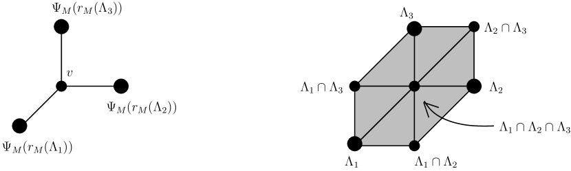
Figure 4. The two iterations of Algorithm 2 for $\Lambda_{1},\Lambda_{2},\Lambda_{3}$ as in Example 24.

Example 24.

We illustrate Algorithm 2 by computing the min-convex hull of three points in the Bruhat–Tits building $\mathcal{B}_{3}$. The input points are given by the three invertible matrices

$$M_{1}\,=\,\begin{pmatrix}z&\!0&\!0\\ 0&\!1&\!0\\ 0&\!0&\!1\end{pmatrix}\!\!,\;M_{2}\,=\,\begin{pmatrix}\!z&\!1&\!1\\ \!0&\!1&\!0\\ \!0&\!0&\!1\end{pmatrix}\!\!,\;M_{3}\,=\,\begin{pmatrix}\!z&\!1&\!4\\ \!0&\!2&\!5\\ \!0&\!3&\!6\end{pmatrix}\!\!.$$

We start with the membrane spanned by $M=(M_{1},M_{2},M_{3})$, and hence with

$$\left(\begin{array}[]{c}\Psi_{M}(r_{M}(\Lambda_{1}))\\ \Psi_{M}(r_{M}(\Lambda_{2}))\\ \Psi_{M}(r_{M}(\Lambda_{3}))\\ \end{array}\right)\,\,\,=\,\,\,\left(\begin{array}[]{ccccccccc}0&0&0&0&-1&-1&0&-1&-1\\ 0&-1&-1&0&0&0&0&-1&-1\\ 0&-1&-1&0&-1&-1&0&0&0\end{array}\right)$$

The tropical convex hull of these three row vectors has precisely one more lattice point:

$$\begin{array}[]{rcl}v&=&(0,-1,-1,0,-1,-1,0,-1,-1)\\ &=&\Psi_{M}(r_{M}(\Lambda_{1}))\,\oplus\,\Psi_{M}(r_{M}(\Lambda_{2}))\\ &=&\Psi_{M}(r_{M}(\Lambda_{1}))\,\oplus\,\Psi_{M}(r_{M}(\Lambda_{3}))\\ &=&\Psi_{M}(r_{M}(\Lambda_{2}))\,\oplus\,\Psi_{M}(r_{M}(\Lambda_{3}))\\ &=&\Psi_{M}(r_{M}(\Lambda_{1}))\,\oplus\,\Psi_{M}(r_{M}(\Lambda_{2}))\,\oplus\,\Psi_{M}(r_{M}(\Lambda_{3})).\end{array}$$

The set $C_{v}$ consists of the vectors $(0,0,a),(0,b,0)$ and $(c,0,0)$ where $a,b,c\in\mathbb{N}$. The unique minimal element is $(0,0,0)$. As its corresponding lattice $\,zR^{3}=\Lambda_{1}\cap\Lambda_{2}\cap\Lambda_{3}\,$ lies in $[M]$, this point adds no new columns to $M^{\prime}$. Since $\Lambda_{1}\cap\Lambda_{2}\cap z^{-1}\Lambda_{3}=\Lambda_{1}\cap\Lambda_{2}\cap z^{-2}\Lambda_{3}$, all lattices $\Lambda_{1}\cap\Lambda_{2}\cap z^{-a}\Lambda_{3}$ are identical for $a\geq 1$. So we can abandon the branch $(0,0,a)$ in $C_{v}$ after $(0,0,1)$. Similarly, we only need to consider up to $(0,1,0)$ and $(1,0,0)$.

After comparing $zR^{3}$ with the lattices $\Lambda_{1}\cap\Lambda_{2}\cap z^{-1}\Lambda_{3}$, $\Lambda_{1}\cap z^{-1}\Lambda_{2}\cap\Lambda_{3}$ and $z^{-1}\Lambda_{1}\cap\Lambda_{2}\cap\Lambda_{3}$ respectively, we augment the columns of $M^{\prime}$ with the three vectors:

$$\begin{array}[]{rcl}(0,1,-1)&\in&(\Lambda_{1}\cap\Lambda_{2}\cap z^{-1}\Lambda_{3})\setminus zR^{3}\\ (0,1,2)&\in&(\Lambda_{1}\cap z^{-1}\Lambda_{2}\cap\Lambda_{3})\setminus zR^{3}\\ (3,2,1)&\in&(z^{-1}\Lambda_{1}\cap\Lambda_{2}\cap\Lambda_{3})\setminus zR^{3}.\\ \end{array}$$

With this new matrix $M^{\prime}$, the images of $\Lambda_{i}$ under the map $\Psi_{M^{\prime}}$ become:

$$\left(\begin{array}[]{c}\Psi_{M^{\prime}}(\Lambda_{1})\\ \Psi_{M^{\prime}}(\Lambda_{2})\\ \Psi_{M^{\prime}}(\Lambda_{3})\\ \end{array}\right)\,\,=\,\,\left(\begin{array}[]{cccccccccccc}0&0&0&0&-1&-1&0&-1&-1&0&0&-1\\ 0&-1&-1&0&0&0&0&-1&-1&0&-1&0\\ 0&-1&-1&0&-1&-1&0&0&0&-1&0&0\end{array}\right)$$

This new membrane $[M^{\prime}]$ contains all the lattices in the min-convex hull of $\Lambda_{1}$, $\Lambda_{2}$, and $\Lambda_{3}$. The tropical convex hull of the three rows contains four other distinct lattice points:

$$\begin{array}[]{rcl}\Psi_{M^{\prime}}(\Lambda_{1}\cap\Lambda_{2})&=&\Psi_{M^{\prime}}(\Lambda_{1})\oplus\Psi_{M^{\prime}}(\Lambda_{2}),\\ \Psi_{M^{\prime}}(\Lambda_{1}\cap\Lambda_{3})&=&\Psi_{M^{\prime}}(\Lambda_{1})\oplus\Psi_{M^{\prime}}(\Lambda_{3}),\\ \Psi_{M^{\prime}}(\Lambda_{2}\cap\Lambda_{3})&=&\Psi_{M^{\prime}}(\Lambda_{2})\oplus\Psi_{M^{\prime}}(\Lambda_{3}),\\ \Psi_{M^{\prime}}(\Lambda_{1}\cap\Lambda_{2}\cap\Lambda_{3})&=&\Psi_{M^{\prime}}(\Lambda_{1})\oplus\Psi_{M^{\prime}}(\Lambda_{2})\oplus\Psi_{M^{\prime}}(\Lambda_{3}).\end{array}$$

The simplicial complex $\,\operatorname{minconv}(\Lambda_{1},\Lambda_{2},\Lambda_{3})\,$ is shown on the right in Figure 4. ∎

Algorithm 2 solves Computational Problem A in the min-convex case. Computing max-convex hulls reduces to computing min-convex hulls, as shown in Algorithm 3.

Input: matrices $M_{1},M_{2},\dots,M_{s}\in\operatorname{GL}_{d}(K)$

Output: $\operatorname{maxconv}(\Lambda_{1},\dots,\Lambda_{s})$ in $\mathcal{B}_{d}$, where $\Lambda_{i}=\operatorname{image}_{R}(M_{i})$

Run Algorithm 2 with input matrices $M_{1}^{-T},\dots,M_{s}^{-T}$.

return $\operatorname{minconv}(\Lambda_{1}^{*},\dots,\Lambda_{s}^{*})$.

Algorithm 3 Max-convex hull in the Bruhat–Tits building $\mathcal{B}_{d}$.

The correctness of Algorithm 3 follows from Lemma 2, which implies that the simplicial complex structure of the max-convex hull of $\Lambda_{1},\ldots,\Lambda_{s}$ is identical to the simplicial complex structure of the min-convex hull of $\Lambda_{1}^{*},\ldots,\Lambda_{s}^{*}$. Our procedure exhibits a matrix of basis vectors for each lattice in $\,\operatorname{minconv}(\Lambda_{1}^{*},\ldots,\Lambda_{s}^{*})$. We take the inverse transpose of that matrix to get a basis matrix for the corresponding lattice in $\,\operatorname{maxconv}(\Lambda_{1},\ldots,\Lambda_{s})$.

5.3. Implementations

We now come to question of how our convex hull algorithms can be used in practice, and what implementations are within reach. We largely focus on the operator “$\operatorname{tconv}$” which is crucial in Algorithm 1, which in turn is called twice in Algorithm 2. Its output form (and hence also the form of the final output of the algorithm) were left deliberately vague, as there are several choices for how “$\operatorname{tconv}$” can be realized. Firstly, there is a direct polyhedral approach for computing tropical convex hulls which is based on the following result from [7, Section 4]: The tropical convex hull of $n$ points in $\mathbb{T}\mathbb{P}^{s-1}$ arises as the polyhedral complex of bounded faces in an ordinary convex polyhedron defined by $ns$ linear inequalities in $\mathbb{R}^{n+s}$. This method is implemented in polymake [11]. The details of this implementation together with extensive tests are the topic of [13]. Secondly, one can use the algebraic algorithm based on resolutions of monomial ideals which was described in [4]. A Macaulay2/Maple implementation is available from the third author. In the planar case, $s=3$, specific techniques from computational geometry can be used to design alternative, faster algorithms; see [15].

In view of tropical polytope duality [7, Theorem 23], we can choose if we want to compute the tropical convex hull of $n$ points in $\mathbb{T}\mathbb{P}^{s-1}$ or of $s$ points in $\mathbb{T}\mathbb{P}^{n-1}$. If $s\leq 3$ then, due to the specialized algorithms mentioned above, it is easier to compute the tropical convex hull of $n$ points in $\mathbb{T}\mathbb{P}^{s-1}$. The output of both, the polyhedral and the algebraic algorithms, returns a tropical polytope $P$ decomposed into cells as in (3).

Enumerating the lattices in Step 2 then requires to list all the lattice points in the ordinary polytopes corresponding to the types. In higher dimensions this can be an arduous task, due to the sheer size of the output. Hence, depending on the application intended, it may be advisable to stick with the output of the previous stage as a compressed description of the set of lattices. From each type we can read off the matroid $M_{u}$ which specifies the set of apartments (spanned by the columns of $M$) containing that type. In Example 3, these matroids $M_{u}$ are the sets of pairs such as $\{af,bf,cf,df,ef,fg,fh\}$.

Table 1. Timings in seconds for computations with “$\operatorname{tconv}$” in polymake. The parameters $d$ and $s$ indicate the size of the problem, that is, computing the min-convex hull of $s$ lattices represented by $d\times d$-matrices. $N$ is the number of samples tested, and the last four columns contain basic statistics.

$d$	$s$	$N$	mean	stddev	$\min$	$\max$
3	2	50	0.18	0.02	0.15	0.21
3	3	50	0.55	0.14	0.31	0.88
3	4	50	2.02	0.94	0.68	5.47
3	5	50	7.73	2.77	2.92	14.25
3	6	50	18.27	8.21	5.40	45.78
3	7	50	38.78	15.21	9.30	77.65
3	8	50	69.39	23.21	30.02	124.05
3	9	50	119.63	41.90	27.66	243.25
3	10	50	231.17	111.22	71.89	594.95
4	2	50	2.75	1.30	0.79	6.07
4	3	50	62.79	42.54	12.20	178.97
4	4	50	827.37	624.19	93.74	3017.19
4	5	18	5994.15	4986.38	648.14	21018.16
4	6	5	35823.43	21936.56	4846.15	67876.56
4	7	5	28266.78	15773.94	9193.69	55891.92

To give a sense of the running time of tropical convex hull code, in Table 1 we list a few timings of polymake computations. The samples were generated at random from $s\times sd$-matrices with integer entries ranging from $0$ to $9$. The algorithm uses the general polyhedral approach without the enumeration of lattice points. The individual timings vary quite a bit, and individual examples with smaller parameters may need more time than other examples with larger parameters. Nonetheless, the reader should get an idea. For more comprehensive tests we refer to [13]. Hardware: AMD 4200+X2, 4423 bogomips, 2GB main memory. Software implemented in polymake 2.3 on SuSE Linux 10.0.

6. Further Algorithms and Perspectives

We now consider Computational Problem B: Determine the intersection of $s$ membranes. The input consists of matrices $M_{1},\ldots,M_{s}$, each having $d$ linearly independent rows over $K=\mathbb{C}(\!(z)\!)$. Here $M_{i}$ represents the membrane $[M_{i}]=[(f_{i1},\dots,f_{id})]$, where $f_{ij}$ is the $j$th column of the matrix $M_{i}$. The intersection $\,[M_{1}]\cap[M_{2}]\cap\dots\cap[M_{s}]\,$ is a locally finite simplicial complex of dimension $\leq d-1$. It may be finite or infinite, depending on the input. We will compute this intersection as a tropical polytope over $(\mathbb{R}\cup\{\infty\},\oplus,\odot)$.

Obviously, $[M_{1}]\cap[M_{2}]\cap\dots\cap[M_{s}]$ is contained in the union $[M_{1}]\cup[M_{2}]\cup\dots\cup[M_{s}]$, which in turn is contained in the membrane $\,[(M_{1},M_{2},\dots,M_{s})]$. By Theorem 18, this membrane is isomorphic, as a simplicial complex, to the standard triangulation of the tropicalization $L_{p}(M)$ of the row space of $M=(M_{1},M_{2},\dots,M_{s})$. In view of Theorem 14, we may regard $L_{p}(M)$ as a polytope in the compactified tropical projective space $\,\overline{\mathbb{T}\mathbb{P}}^{sd-1}$.

Our computations take place inside this tropical linear space $L_{p}(M)$, which we represent as the tropical convex hull of the cocircuits $\,p(\sigma*)\,$ that are derived from the matrix $M$. The $k$-th column vector $f_{ik}$ of the $i$-th input matrix $M_{i}$ corresponds to the cocircuit $\,p(\sigma*)\,$ where $\sigma$ is the $(d{-}1)$-subset of $\{1,2,\ldots,sd\}$ which indexes all columns of $M_{i}$ other than $f_{ik}$ inside $M$. This special cocircuit is abbreviated by $\,C_{ik}\,:=\,\operatorname{val}\bigl{(}\,\text{the $k$-th row $M_{i}^{-1}\cdot M$}\,\bigr{)}$. Consider the subpolytope of $L_{p}(M)$ spanned by the $d$ special cocircuits arising from $M_{i}$:

$$L_{p}^{M}(M_{i})\quad=\quad\operatorname{tconv}\{C_{i1},\ldots,C_{id}\}.$$

This tropical polytope with its standard triangulation is isomorphic to the membrane $[M_{i}]$. Intersecting these subpolytopes $L_{p}(M_{i})$ inside $L_{p}(M)$ solves Computational Problem $B$.

The intersections of arbitrary tropical polytopes are tropical polytopes again [7, Proposition 20]. Here, however, the situation is even easier since the subpolytope $L_{p}^{M}(M_{i})$, as an ordinary polytopal complex, is a subcomplex of $L_{p}(M)$. We summarize our findings in Algorithm 4. Our remarks concerning the output of Algorithm 2 apply accordingly.

Input: Matrices $M_{1},M_{2},\dots,M_{s}\in\operatorname{GL}_{d}(K)$

Output: Intersection $[M_{1}]\cap[M_{2}]\cap\dots\cap[M_{s}]$ of membranes in $\mathcal{B}_{d}$

$M\leftarrow(M_{1},M_{2},\dots,M_{s})$

$C\leftarrow sd\times sd\text{-matrix of cocircuits of }M$

$L_{p}(M)\leftarrow\operatorname{tconv}\{c_{11},\dots,c_{ss}\}$

for $k\leftarrow 1,2,\dots,s$ do  $L_{p}^{M}(M_{i})\leftarrow\operatorname{tconv}\{c_{i1},\dots,c_{id}\}$

  $I\leftarrow\emptyset$

foreach cell $C$ in $L_{p}(M)$ do  if $C\subseteq L_{p}^{M}(M_{i})$ for all $i$ then  $I\leftarrow I\cup C$

    return $I$

Algorithm 4 Intersection of membranes in the affine building $\mathcal{B}_{d}$

We now examine the special case of Computational Problem B where each input matrix $M_{i}$ is square. Here our problem is to compute the intersection of $s$ apartments in $\mathcal{B}_{d}$. Since apartments are both min- and max-convex, the intersection of apartments is also min- and max-convex. This establishes the connection between Computational Problem B and the classical notion of convexity in Remark 6. The set of all chambers which are fully contained in the intersection of apartments is convex in the sense of Remark 6. Note that (the vertex set of) every convex set of chambers within some apartment of $\mathcal{B}_{d}$ arises in this manner, namely as the output of Algorithm 4 for some square matrices $M_{1},\ldots,M_{s}$. Identifying one of the apartments with $\mathbb{T}\mathbb{P}^{d-1}$, we see that the result of this computation is a subset of $\mathbb{T}\mathbb{P}^{d-1}$ which is both min-convex and max-convex. This implies that the intersection of apartments is an ordinary convex polytope of the special form (3).

Recent work of Alessandrini [2] suggests the following alternative method this computation, which more efficient than applying Algorithm 4 to square matrices. Our point of departure towards Alessandrini’s method is the following question: Given $M\in\operatorname{GL}_{d}(K)$, how can we decide whether the standard lattice $R^{d}$ lies in the apartment $[M]$, i.e. whether $R^{d}$ has an $R$-basis of the form $\{z^{a_{1}}f_{1},z^{a_{2}}f_{2},....,z^{a_{d}}f_{d}\}$ for some integers $a_{1},a_{2},\ldots,a_{d}$?

To answer this question, we compute the tropical $d\times d$-matrix

(12) $$E(M)\quad:=\quad\operatorname{val}(M)\odot\operatorname{val}(M^{-1})\,.$$

Here $\odot$ means that the matrix product is evaluated in the min-plus algebra. Note that each diagonal entry of $E(M)$ is non-negative. The following lemma is easy to derive:

Lemma 25.

The following are equivalent for a matrix $M\in\operatorname{GL}_{d}(K)$:

1. The standard lattice $R^{d}$ lies in the apartment $[M]$.

2. By scaling the columns of $M$ with powers of $z$, we can get a matrix $G$ in $R^{d\times d}$ whose constant term $G(0)\in\mathbb{C}^{d\times d}$ is invertible.

3. Each entry $e_{ij}(M)$ of the matrix E(M) is non-negative.

We now change the question as follows. Let $u_{1},\ldots,u_{d}$ be unknown integers. Under what condition on these integers is the scaled standard lattice $R\{z^{u_{1}}e_{1},...,z^{u_{d}}e_{d}\}$ in the apartment $[M]$? This question is equivalent to asking whether the standard lattice $R^{d}$ lies in the apartment $\,[\,\operatorname{diag}(z^{-u})\cdot M\,]$, where $\operatorname{diag}(z^{-u})=\operatorname{diag}(z^{-u_{1}},\ldots,z^{-u_{d}})$. By applying Lemma 25 to the matrix $\,\operatorname{diag}(z^{-u})\cdot M\,$ in place of $M$, we obtain the following result.

Corollary 26.

The lattice $R\{z^{u_{1}}e_{1},...,z^{u_{d}}e_{d}\}$ lies in the apartment $[M]$ if and only if

(13) $$u_{j}-u_{i}\,\,\leq\,\,e_{ij}(M)\qquad\hbox{for}\,\,\,i,j=1,2,\ldots,d.$$

The linear inequalities (13) in the unknowns $u_{1},\ldots,u_{d}$ defines a convex subset of $\mathbb{T}\mathbb{P}^{d-1}$ which is both an ordinary polytope and a tropical polytope. Corollary 26 is essentially equivalent to Theorem 4.7 in [2]. Alessandrini refers to the polytope (13) as the inversion domain associated with the tropical matrix product in (12); see [2, Proposition 3.4]. We conclude that the intersection of the two apartments $[M]$ and $[\operatorname{diag}(1,\ldots,1)]$ equals the standard triangulation of the inversion domain, which is specified by the inequalities (13).

We now present our second method, to be called Alessandrini’s Algorithm, for Computational Problem B in the special case of apartments. The input consists of $s$ invertible matrices $M_{1},M_{2},\dots,M_{s}$ over $K$, and the output is the intersection $[M_{1}]\cap\dots\cap[M_{s}]$ of apartments. After multiplying each matrix on the left by $M_{1}^{-1}$, we may assume that $M_{1}$ is the identity matrix. Then the desired intersection is the standard triangulation of the polytope specified by the inequalities (13) where $M$ runs over $\{M_{2},\dots,M_{k}\}$. Alessandrini’s Algorithm is summarized by the following refinement of Proposition 20.

Theorem 27.

The intersection of apartments $[M_{1}]\cap\cdots\cap[M_{s}]$ in the Bruhat–Tits building $\mathcal{B}_{d}$ is the standard triangulation of a polytope of the form (3), namely, the polytope

$$\left\{\,u\in\mathbb{T}\mathbb{P}^{d-1}\vphantom{u_{j}-u_{i}\leq e_{ij}(M_{k})\text{ for }i,j=1,\dots,d\text{ and }k=2,\dots,s}\,:\,\vphantom{u\in\mathbb{T}\mathbb{P}^{d-1}}u_{j}-u_{i}\leq e_{ij}(M_{k})\text{ for }i,j=1,\dots,d\text{ and }k=2,\dots,s\,\right\}\,.$$

Conclusion

We have demonstrated that tropical convexity is a useful tool for computations with affine buildings. Given the ubiquitous appearance of affine buildings in mathematics, we are optimistic that our approach can be of interest for a wide range of applications. Such applications may arise in fields as diverse as geometric topology [2], number theory [10, 21], algebraic geometry [16, 17], representation theory [12], harmonic analysis [19], and differential equations [6]. Experts in combinatorial representation theory may find it interesting to generalize our constructions and algorithms to affine buildings of other types. This will require to investigate, for instance, the $B_{n}$-analogs of tropical polytopes.

References

- [1] Peter Abramenko and Kenneth S. Brown, Approaches to Buildings, Springer-Verlag, New York, 2007.
- [2] Daniele Alessandrini, Tropicalization of group representations, arXiv:math.GT/0703608.
- [3] Federico Ardila, Subdominant matroid ultrametrics, Annals of Combinatorics 8 (2004) 379–389.
- [4] Florian Block and Josephine Yu, Tropical convexity via cellular resolutions, J. Algebraic Combin. 24 (2006), no. 1, 103–114.
- [5] François Bruhat and Jacques Tits, -paires de type affine et données radicielles, C. R. Acad. Sci. Paris Sér. A-B 263 (1966), A598–A601.
- [6] Eduardo Corel, Moser-reduction of lattices for a linear connection, preprint, 2007, www.math.jussieu.fr/~corel/publications/publi-list.html.
- [7] Mike Develin and Bernd Sturmfels, Tropical convexity, Doc. Math. 9 (2004), 1–27 (electronic).
- [8] Andreas Dress and Werner Terhalle, A combinatorial approach to -adic geometry, Geom. Dedicata 46 (1993), no. 2, 127–148.
- [9] by same author, The tree of life and other affine buildings, Proceedings of the International Congress of Mathematicians, Vol. III (Berlin, 1998), Extra Vol. III, 1998, pp. 565–574 (electronic).
- [10] Gerd Faltings, Toroidal resolutions for some matrix singularities, Moduli of abelian varieties (Texel Island, 1999), Progr. Math., vol. 195, Birkhäuser, Basel, 2001, pp. 157–184.
- [11] Ewgenij Gawrilow and Michael Joswig, polymake: a framework for analyzing convex polytopes, Polytopes—combinatorics and computation (Oberwolfach, 1997), DMV Sem., vol. 29, Birkhäuser, Basel, 2000, pp. 43–73.
- [12] Ulrich Goertz, Alcove walks and nearby cycles on affine flag manifolds, to appear in the Journal of Algebraic Combinatorics, arXiv:math.RT/0610839.
- [13] Sven Herrmann, Michael Joswig, and Marc E. Pfetsch, Computing the bounded subcomplex of an unbounded polyhedron, in preparation.
- [14] Petra Hitzelberger, A convexity theorem for affine buildings, arXiv:math.MG/0701094.
- [15] Michael Joswig, Tropical halfspaces, Combinatorial and computational geometry, Math. Sci. Res. Inst. Publ., vol. 52, Cambridge Univ. Press, Cambridge, 2005, pp. 409–431.
- [16] Mikhail M. Kapranov, Chow quotients of Grassmannians. I, I. M. Gel′fand Seminar, Adv. Soviet Math., vol. 16, Amer. Math. Soc., Providence, RI, 1993, pp. 29–110.
- [17] Sean Keel and Jenia Tevelev, Geometry of Chow quotients of Grassmannians, Duke Math. J. 134 (2006), no. 2, 259–311.
- [18] G. A. Mustafin, Non-Archimedean uniformization, Mat. Sb. (N.S.) 34 (1978), no. 2, 187–214.
- [19] James Parkinson, Spherical harmonic analysis on affine buildings, arXiv:math.FA/0604058.
- [20] Jürgen Richter-Gebert, Bernd Sturmfels and Thorsten Theobald, First steps in tropical geometry, in ”Idempotent Mathematics and Mathematical Physics”, Proceedings Vienna 2003, (editors G.L. Litvinov, V.P. Maslov), American Math. Society, Contemporary Mathematics 377 (2005) 289-317.
- [21] Alison Setyadi, Distance in the Affine Buildings of and , arXiv:math.NT/0511556
- [22] David Speyer, Tropical linear spaces, arXiv:math.CO/0410455.
- [23] David Speyer and Bernd Sturmfels, The tropical Grassmannian, Adv. in Geometry 4 (2004) 389-411.
- [24] Jacques Tits, Buildings of spherical type and finite BN-pairs, Springer-Verlag, Berlin, 1974, Lecture Notes in Mathematics, Vol. 386.
- [25] Annette Werner, Compactification of the Bruhat-Tits building of PGL by lattices of smaller rank, Doc. Math. 6 (2001), 315–341 (electronic).
- [26] by same author, Compactification of the Bruhat-Tits building of PGL by seminorms, Math. Z. 248 (2004), no. 3, 511–526.
- [27] Josephine Yu and Debbie S. Yuster, Representing tropical linear spaces by circuits, arXiv:math.CO/0611579.