Propagation of travelling waves in sub-excitable systems driven by noise and periodic forcing

Abstract

It has been reported that traveling waves propagate periodically and stably in sub-excitable systems driven by noise [Phys. Rev. Lett. 88, 138301 (2002)]. As a further investigation, here we observe different types of traveling waves under different noises and periodic forces, using a simplified Oregonator model. Depending on different noises and periodic forces, we have observed different types of wave propagation (or their disappearance). Moreover, the reversal phenomena are observed in this system based on the numerical experiments in the one-dimensional space. As an explanation, we regard it as the effect of periodic forces. Thus, we give qualitative explanations to how reversal phenomena stably appear, which seem to arise from the mixing function of the periodic force and the noise. And the output period and three velocities (the normal, the positive and the negative) of the travelling waves are defined and their relationship with the periodic forces, along with the types of waves, are also studied in sub-excitable system under a fixed noise intensity.

1 Introduction

The effects of noise on nonlinear systems are the subject of intense experimental and theoretical investigations. Noise can induce transition Horsthemke ; RM2006 , bifurcations 1742-5468-2007-07-P07016 , and stochastic resonance Gammaitoni ; Hz1998 ; KW1995 ; PhysRevLett.74.2130 . Especially, in Ref. PhysRevLett.74.2130 the synchronization of spatiotemporal patterns were observed in an excitable medium by the numerical evidence. Moreover noise can enhance propagation in arrays of coupled bistable oscillators Lindner ; PhysRevLett.76.2609 ; PhysRevE.54.3479 ; PhysRevA.38.983 . In an excitable system, an external periodic forcing can dramatically change its behavior. As reported by previous documents, the phase locking, quasi-periodicity, period doubling, and chaos were observed Feingold . The temporal evolution of the concentration patterns has been modeled by partial differential reaction-diffusion equations. Such models include oscillatory, excitable or bistable systems with either none, one or two linearly stable homogeneous states meron ; Mikhailov . It is also well known that in sub-excitable systems noise also can induce travelling waves Kadar , drive avalanche behavior Wang , and sustain pulsating patterns and global oscillations PhysRevLett.82.3713 . Sub-excitable systems under noises and periodic forcing are able to send out travelling and spiral waves. Belousov-Zhabotinsky (BZ) reaction Zakin ; Field is a popular symbol in nonlinear dynamical realm to study excitable and sub-excitable system. It has been widely agreed that the noise and periodic forcing play a very important role in wave propagation and stability.

Recently, it was observed that noise can support wave propagations in sub-excitable Zhou2002 ; PhysRevLett.82.3713 ; Kadar systems due to a noise-induced transition PhysRevLett.87.078302 ; Garcia-Ojalvo . In these studied, the medias are static, and transports are governed by diffusion 1742-5468-2007-07-P07013 . However in many situations, the medias are not static but subject to a motion. For example, stirred by a flow, or by the periodic forcing, the convective-like phenomena were observed due to electric field in Ref. PhysRevLett.76.3854 , which occurs especially in chemical reactions in a fluid environment. In such cases, diffusive transport usually dominates only at small spatial scales while mixing due to the flow in much faster at large scale. In Refs. PhysRevLett.91.084101 ; PhysRevE.66.066208 ; 1367-2630-7-1-018 , the authors shown that in an inhomogeneous self-sustained oscillatory media, an increasing rate of mixing can lead to a transition to a global synchronization of the whole media. Especially, Ref. PhysRevLett.91.150601 showed that the interplay among excitability, noise, diffusion and mixing can generate various pattern formation in a 2D FigzHugh-Nagumo (FHN) model subject to the advection by a chaotic flow. Here, we research the effect of noise and periodic forcing on sub-excitable systems using the Oregonator model in one dimension, which advances from the BZ reaction. The reversal phenomenon is not observed in the previous documents about the propagation of travelling waves. It is founded in this paper, which relates to a new concept. In Ref. Albanese , Richard A. Albanese refers to reversal concept in wave propagation concern extraction of information about distant structural features from the measurements of scattered waves, but it is irrelevant the excitable system.

In our paper, we define that the general traveling waves propagate forward in one constant direction and vice versa. Under this definition, we found the reversal phenomena in our numerical simulations. However in our simulation we have discovered that after some time, the waves change its propagation direction and turn backward to travel in the opposite direction. The traveling waves propagate forward and backward alternately and periodically. That is called the reversal phenomenon (see the supplementary material on-line movie for this phenomenon, Movie-0). In the mathematical language, the definition of definition of an “reversal phenomenon” as at time $t$, the spatial position of a traveling wave front is at point $x$. After some time $\Delta t>0$, the wave front reaches point $x$ again with reversal direction. In fact, this phenomenon was observed in the FHN model by numerical simulations PhysRevLett.91.150601 . In this article, our focuses are the effect of the periodic forcing and noise on the propagation of traveling waves in sub-excitable systems.

2 Model

Most of the systems we are interested in reside in a d-dimensional world. This means that our variables (fields or concentrations) depend on time and space. In present paper, the starting deterministic model Zhou2002 is based on partial differential equations, and when the randomness is introduced we transform them into stochastic partial differential equation. A representative example is the deterministic reaction-diffusion equation,

$$\frac{\partial\phi({\bf x},t)}{\partial t}=f(\phi({\bf x},t),\mu)+\mathcal{D}\nabla^{2}\phi({\bf x},t),$$ (1)

where $\phi({\bf x},t)$ represent the density of a physical observable, $f(\phi({\bf x},t),\mu)$ is a nonlinear function of the field $\phi$ and $\mu$ denotes the relevant control parameter. The above equation can be made more complicated when considering vector fields, higher-order derivatives, or nonlocal operators. The effect of fluctuations is introduced through a stochastic process or noise $\xi({\bf x},t)$ with well controlled statistical properties. As a result, we expect that the new equation governing our system will have the generic form

$$\frac{\partial\phi({\bf x},t)}{\partial t}=f(\phi({\bf x},t),\mu)+\mathcal{D}\nabla^{2}\phi({\bf x},t)+g(\phi)\xi({\bf x},t).$$ (2)

We take into account this standard example of stochastic partial differential equation and the two-variable Oregonator model Field ; Tyson that is famous for its convenience to study the property of diffusion-reaction systems. Our modified model adds both noise and the periodic forces, which is,

$$\frac{\partial u}{\partial t}=\frac{1}{\varepsilon}f(u,v)+D_{u}\nabla^{2}u+(D_{\rm s}\xi(t)+E(t))\frac{\partial u}{\partial x},$$ (3a)

$$\frac{\partial v}{\partial t}=g(u,v)+D_{v}\nabla^{2}v+(D_{\rm s}\xi(t)+E(t))\frac{\partial v}{\partial x},$$ (3b)

where $f(u,v)=u(1-u)-fv\frac{u-q}{u+q}$, and $g(u,v)=u-v$. $\nabla^{2}$ is the Laplacian operator in Cartesian coordinates. $u$ and $v$ represent the concentration of $\rm HBrO_{2}$ and the catalyst $2\textrm{Ce}^{4+}$, respectively. Here, the external electric field can be considered as a spatially uniform electric field, which includes two parts: stochastic forcing, $\xi(t)$ (we use the notation of $\xi(t)$ for irrelevant in space) and the periodic force , $E(t)$. Both of them depend on time $t$ with the form of Gaussian noise and with the periodic function respectively. $\xi(t)$ denotes Gaussian white noise with $\langle\xi(t)\rangle=0$ and $\langle\xi(t)\xi(t^{{}^{\prime}})\rangle=2D_{\rm s}\delta(t-t^{\prime})$, a typical temporally varied Gaussian white noise and here $D_{\rm s}$ is the intensity of noise. $E(t)$ is the periodic force, where the sine periodic force is chosen, $E(t)=F\sin(\frac{2\pi}{T_{\rm in}}t)$. $F$ and $T_{\rm in}$ are the intensity of the periodic forcing and the input period, respectively. The effect of electric field is convective-like, as discussed in Ref. PhysRevLett.76.3854 . $D_{u}$ and $D_{v}$ are the dimensionless diffusion coefficients of $u$ and $v$, $D_{u}=1.0$, $D_{v}=0.6$ Jahnke .

The dynamical system (3) is simulated in one-dimensional space by Euler-Maruyama Method DJHigham with zero flux boundary conditions on a space length of $500$ elements. The space step is $\Delta x=0.15$ space unit and the time step is $\Delta t=10^{-3}$ time unit. These parameters are chosen to make the simulation process relatively stable and the information of wave propagation can be relatively all-around. In order to avoid the simulation going to the negative region of $u$, we let $u>q$, if $u<q$, $u=q$, according to the method of the Refs. Skaggs ; Winfree . The simulations have been done as follows: we excite $3$ elements at the left boundary in the our systems under sub-excitable state in the one-dimensional space, which serves as the wave source. The leapfrog method for the advection terms; an implicit method for the diffusion terms; and a simple explicit Euler method for the reaction terms. Letting $U_{j}^{n}\approx u(x_{j},t_{n})$ and $V_{j}^{n}\approx v(x_{j},t_{n})$, where $x_{j+1}-x_{j}=\Delta x$ and $t^{n+1}-t^{n}=\Delta t$, results in the following discretised system:

$$\frac{U_{j}^{n+1}-U_{j}^{n}}{\Delta t} = \frac{1}{\varepsilon}f(U_{j}^{n},V_{j}^{n})+D_{u}\Big{[}\frac{U_{j+1}^{n+1}-2U_{j}^{n+1}+U_{j-1}^{n+1}}{(\Delta x)^{2}}\Big{]}$$ (4)

$$+(D_{\rm s}\xi(t)+E(t))\Big{[}\frac{U_{j+1}^{n}-U_{j-1}^{n}}{2\Delta x}\Big{]},$$

$$\frac{V_{j}^{n+1}-V_{j}^{n}}{\Delta t} = g(U_{j}^{n},V_{j}^{n})+D_{v}\Big{[}\frac{V_{j+1}^{n+1}-2V_{j}^{n+1}+V_{j-1}^{n+1}}{(\Delta x)^{2}}\Big{]}$$

$$+(D_{\rm s}\xi(t)+E(t))\Big{[}\frac{V_{j+1}^{n}-V_{j-1}^{n}}{2\Delta x}\Big{]},$$

where $D_{\rm s}$, $F$, and $T_{\rm in}$ are the control parameters. Note that here the noise term $\xi(t)$ is Gaussian and white. This is a very reasonable assumption for internal noise, which represents many irrelevant degrees of freedom evolving very short temporal and spatial scales. It has a probability density function of the normal distribution (also known as Gaussian distribution). In other words, the values that the noise can take on are Gaussian distributed.

3 Result

Extensive testing is performed through numerical simulations to the described model (3) and the qualitative results are shown this section.

3.1 Sub-excitation and reversal phenomena

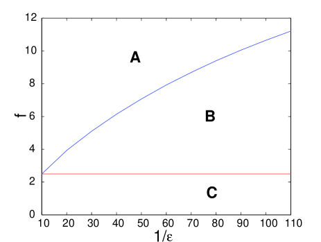
Figure 1: (Color online) The phase diagram of the $\varepsilon$ versus $f$.

$q$, $\epsilon$ and $f$ are parameters related to the BZ kinetics, determining the sub-excitation of the system. $q=0.002$ Tyson . First we simulate the dynamical system (3) without noise and periodic force to confirm the sub-excitable region. The result is shown in Fig. 1. In region (A) no traveling waves are produced in the system; in region (B) traveling waves are sent out and propagating in the system; region (C) is not included in the excitable confine. In the area between region (A) and (B), traveling waves are sent out but die away gradually, which is so-called the sub-excitable region, corresponding to the blue line in Fig. 1. Here we set $\epsilon=0.1$ and $f=2.435$ to fix our system into in a sub-excitable region. When the parameters $\epsilon$ and $f$ are deeply in the sub-excitable domain, the same results are observed by the numerical experiments, such as, $\epsilon=0.025$, $f=2.435$ and $\epsilon=0.025$, $f=4.0$.

It turns out that the influence of noise is rather important in the sub-excitable media. There is an extreme case for the system (3), that is, when the intensity of noise equals to $0$, i.e. $D_{\rm s}=0$, and only the periodic force is present, the different types of wave propagation are summarized in the Table 1. Table 1 reveals that there exists critical input period $T_{\rm in}^{*}$ for each intensity of periodic force $F$ ($F>10.0$), so that the system creates traveling waves periodically and waves propagate persistently. If $F<10.0$, the system can only send out one wave, and there is no critical input period $T_{\rm in}^{*}$; The system sends out traveling waves periodically but the waves disappear quickly when the $T_{\rm in}>T_{\rm in}^{*}$ (see Movie-1 for this case, where $D_{\rm s}=0$, $T_{\rm in}=8.0$, and $F=10.0$); when $F=10.0$, $T_{\rm in}^{*}=5.0$; $F=20.0$, $T_{\rm in}^{*}=4.0,5.0$; $F=30.0$, $T_{\rm in}^{*}=3.0,4.0,5.0$.

Table 1: Traveling waves propagation under different $F$ and $T_{\rm in}$ with noise intensity $D_{\rm s}=0$; symbol $-1$ indicates the system sends out only one wave; symbol $-$ indicates the system sends out traveling waves periodically but the waves disappear quickly; symbol $+$ indicates the system sends out traveling waves periodically and the waves can propagate persistently.

	$T_{\rm in}<2.0$	$T_{\rm in}=2.0$	$T_{\rm in}=3.0$	$T_{\rm in}=4.3$	$T_{\rm in}=5.0$	$T_{\rm in}=6.0$	$T_{\rm in}>6.0$
$F<10.0$	$-1$	$-1$	$-1$	$-$	$-$	$-$	$-$
$F=10.0$	$-1$	$-1$	$-1$	$-1$	$+$	$-$	$-$
$F=20.0$	$-1$	$-1$	$-1$	$+$	$+$	$-$	$-$
$F=30.0$	$-1$	$-1$	$+$	$+$	$+$	$-$	$-$

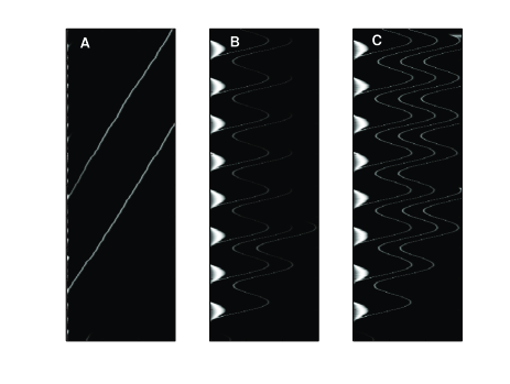
Figure 2: (Color online) The spatiotemporal plot of the variable $u$ for the system (3), where the ordinate is time evolution and the abscissa represents the spatial location. The white part indicates wave front. (A) only noise present, $D_{\rm s}=14.0$, and $F=0$ (see the Movie-2, additional movies format available from Journal Web); (B) Both noise and periodic forcing present, $D_{\rm s}=10.0$, $F=10.0$, and $T_{\rm in}=8.0$ (see the Movie-3, additional movies format available from Journal Web); (C) Both noise and periodic forcing present, $D_{\rm s}=14.0$, $F=10.0$, and $T_{\rm in}=8.0$ (see the Movie-4, additional movies format available from Journal Web).

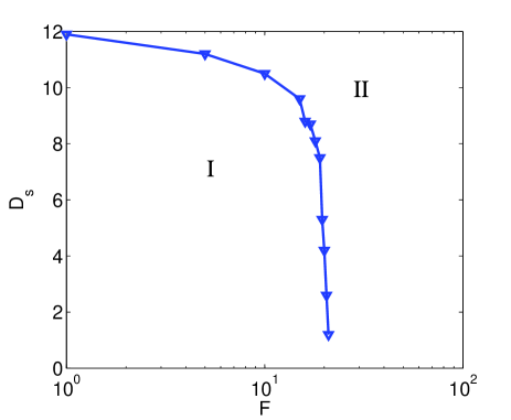
Figure 3: (Color online) Phase diagram about the reversal phenomena with respect to $D_{\rm s}$–$F$ parameter space. The parameters are the same as Fig. 2, but $T_{\rm in}=8.0$. The reversal waves will die out quickly within region I and propagate persistently within region II. Note that the log scale for $T_{\rm in}$. ($\blacktriangledown$, the critical values from simulation results.)

Now, we turn on the noise and the periodic forces in the system (3) and investigate their effects when the intensity of noise takes different values. Fig. 2 shows that traveling waves propagate with different noise and periodic forces. The abscissa is the spatial location and the ordinate is the evolution of time. The white part indicates wave crests. As shown in Fig. 2(A), if only noise present, traveling waves are produced irregularly but they can propagate stably [see Movie-2]. If periodic force and noise both present, travelling waves are produced periodically and reversal phenomena appear, however traveling waves die out quickly when the intensity of noise is small [see Movie-3]. The travelling waves are produced periodically and they propagate stably, and reversal phenomena also appear when the intensity of noise is increased [see Movie-4], as shown in Fig. 2(C). In Fig. 3, we show the phase diagram about the reversal phenomena with respect to the $D_{\rm s}$–$F$ parameter space, in which the reversal travelling waves will die out quickly within the region I but propagate persistently within the region II. One can see that the reversal waves sensitively depend on the intensity of periodic forces and the noise intensities for the fixing $T_{in}$. For example (see Fig. 3), the emergence of reversal waves is a sensitive relationship at before and after the certain critical value. For the large $F$, the curve is sharp decreasing, otherwise the cure is slow decreasing. So we can obtain conclusion from Figs. 2 and 3, that the stabilization of traveling waves are due to noise, but the periodicity owe to the function of periodic force. Periodical and stable traveling waves, as well as reversal phenomena, are produced in sub-excitable system driven by noise and periodic force.

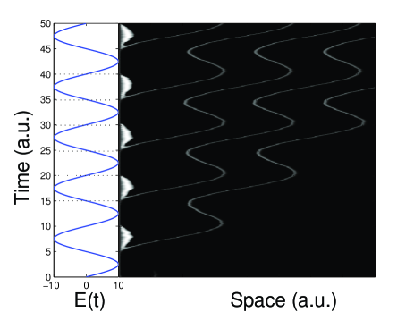
Figure 4: (Color online) The propagation of traveling waves with the periodic force $E(t)=F\sin(\frac{2\pi}{T_{\rm in}}t)$. The ordinate is time evolution. For the left window the abscissa represents $E(t)$ and for the right the abscissa is space location. The left and right window share the same ordinate which is time. The parameters are $D_{\rm s}=14.0$, $F=10.0$, and $T_{\rm in}=8.0$.

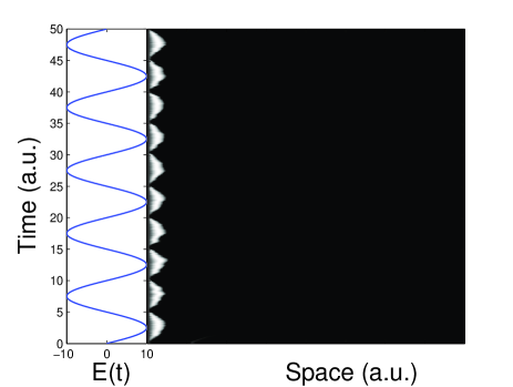
Figure 5: (Color online) The propagation of travelling waves with the periodic forcing $E(t)=E_{-}(t)$ (or $E(t)=E_{+}(t)$). The ordinate is time evolution. For the left window the abscissa represents $E(t)$ and for the right the abscissa is space location. The left and right window share the same ordinate which is time. The parameters are $D_{\rm s}=14.0$, $F=10.0$, and $T_{\rm in}=8.0$.

To characterize the relation between the periodic force and reversal phenomena, we give some qualitative explanations. Fig. 4 shows the relationship between the propagation of traveling waves with the periodic force $E(t)=F\sin(\frac{2\pi}{T_{\rm in}}t)$. The left window of Fig. 4 is the periodic force whose abscissa is $E(t)$ and the right window represents the spatiotemporal plot of variable $u$ whose abscissa is the spatial location. The left and right window share the same ordinate which is time. From Fig. 4 we can easily obtain that corresponding to each input period the system sends out a traveling wave, which is $1:1$ frequency locking. The dotted line in the left window of Fig. 4 divide out the positive and negative parts of the periodic force. We find out that if the periodic force is negative, traveling waves propagate forward, whereas if the periodic force is positive, traveling waves propagate backward in the opposite direction. Thus reversal phenomena appear.

For further investigation, we test several different kinds of periodic force for system (3). They are $E_{\sqcap}(t)=(-1)^{\lfloor\frac{2t}{T_{\rm in}}\rfloor}F$ (the rectangle periodic force, here the $\lfloor n\rfloor$ denotes the integer of the $n$), $E_{-}(t)=-|F\sin(\frac{2\pi}{T_{\rm in}}t)|$ and $E_{+}(t)=|F\sin(\frac{2\pi}{T_{\rm in}}t)|$. When the periodic forcing is $E_{\sqcap}(t)$, travelling waves are produced periodically and they propagate stably, and reversal phenomena appear (resemble the Fig. 2(C)). When the periodic force is $E_{-}(t)$ or $E_{+}(t)$, there are only foundations formed but no travelling waves are sent out, as shown in Fig. 5. So the reversal phenomenon is due to the alternation of the positive and negative values of the periodic force. If each value of the periodic force was positive (or negative), no travelling waves will be sent out and of course no reversal phenomena will appear.

3.2 The output period and the three velocities

In this section we focus on the effect of the periodic force $E(t)=F\sin(\frac{2\pi}{T_{\rm in}}t)$ on the propagation of travelling waves. Here, the noise intensity $D_{\rm s}$ is fixed at 14.0. Furthermore, we define several quantities of the traveling waves. The output period $T_{\rm out}$ is defined as follows: $T_{i}$ is the time interval between the $i$th wave and the $i+1$th wave. $m$ waves are taken into account and the average value of them is $T_{\rm out}$, where $T_{\rm out}=\frac{\sum\limits_{i=1}^{m}T_{i}}{m-1}$. The three velocities (the normal, the positive and the negative) of the traveling waves are defined as follows: when traveling waves propagate forward, there is a mean propagation velocity which is the positive velocity, and denoted by $V_{+}$. The mean velocity of the backward propagating waves is likewise denoted by $V_{-}$. In addition, $V$ is defined here as the average velocity of the whole propagation of traveling wave. The output period $T_{\rm out}$, the normal velocity $V$, the positive velocity $V_{+}$ and the negative velocity $V_{-}$ are shown in Fig. 6. The slopes of the red, blue and yellow lines in Fig. 6 are $1/V$, $1/V_{+}$ and $1/V_{-}$, respectively.

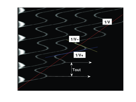
Figure 6: (Color online) The sketch map of $T_{\rm out}$, $V$, $V_{+}$, and $V_{-}$ with $D_{\rm s}=14.0,F=10.0,T_{\rm in}=8.0$.

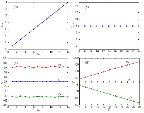
Figure 7: (Color online) The effect of periodic force on the property of traveling waves, $D_{\rm s}=14.0$. (a) The plot of the output period with respect to the input period, $F=10.0$. (b) The plot of the output period with respect to the intensity of periodic force, $T_{\rm in}=8.0$. (c) The plot of the three velocities of the traveling waves with respect to the input period, and $F=10.0$. (d) The plot of the three velocities of the traveling waves with respect to the intensity of periodic force, $T_{\rm in}=8.0$.

Based on the definition, we now focus our simulations on the relationship between periodic force and the properties of travelling waves. The results are shown in Fig. 7. Above all we interpret how the periodic force $E(t)$ affects the output period $T_{\rm out}$. First, we fix $F=10.0$ (the intensity of the periodic force) and study how $T_{\rm out}$ changes with $T_{\rm in}$ (the input period),as shown in Fig. 7(a). One observes that the output period increases linearly with the input period. Moreover, the output period is the same as the input period (the slope equals to $1$). Second, we fix $T_{\rm in}=8.0$ and study the relation between $T_{\rm out}$ and $F$, as shown in Fig. 7(b), from which one observes that the output period is a constant and independent of the intensity of the period forcing. So we can draw a conclusion that the output period is the same as the input period and is independent of the intensity of the periodic force, under a fixed noise intensity.

Next we investigate the influence of the periodic force $E(t)$ on the three velocities of the travelling waves (the normal $V$, the positive $V_{+}$ and the negative $V_{-}$). First we fix the intensity of the period forcing $F=10.0$ and see the changes of $V$, $V_{+}$, and $V_{-}$ with the input period $T_{\rm in}$, respectively. The results are shown in Fig. 7(c), from which we observe that the normal, positive and negative velocities approximate constant values, respectively, independent of the input period. Then we fix $T_{\rm in}=8.0$ and study the changes of $V$, $V_{+}$ and $V_{-}$ with $F$ (see Fig. 7(d)), which shows that the normal velocity is constant independent of the intensity of the periodic forcing; the positive velocity increases with the intensity of periodic force, while the negative velocity decreases with the intensity of periodic force. So we can conclude that the normal velocity is independent of the periodic force; the positive the negative velocities have the same trend with the intensity of periodic forces and do not depend on the input period.

It is natural to presume from the above results that the three velocities are interrelated. Through quantities of data, we obtain the relationship among the normal, positive and negative velocities, as follows

$$2V=V_{+}+V_{-},$$ (6)

that is,

$$V^{*}=V_{+}-V=V-V_{-}.$$ (7)

So the positive velocity is the normal velocity plus the $V^{*}$, and the negative velocity is the normal velocity minus the $V^{*}$.

4 conclusion and discussion

In conclusion, noise and periodic force play a very important role on the production, propagation, and stability of the traveling waves in sub-excitable systems. Noise can induce traveling waves to propagate stably. It can also support wave propagation in sub-excitable Zhou2002 ; PhysRevLett.82.3713 ; Kadar media due to a noise-induced transition PhysRevLett.87.078302 ; Garcia-Ojalvo ; Francesc . In these studies, the media are static, and transport is governed by diffusion. In many systems, the media are not static, but subject to a motion, for example, when stirred by a flow, or by the oscillatory electric field (with period). This occurs especially in chemical reactions in a fluid environment. In this case, usually diffusive transport dominates only at small spatial scales while mixing due to the flow in much faster at large scale. In this paper, we investigate the sub-excitable system using a simplified Oregonator model, and the propagation of traveling waves in the presence of both noise and periodic force. Depending on noise and the periodic forcing we have observed different types of wave propagation (or its disappearance). Moreover, the reversal phenomena is observed in this system based on the numerical experiments in one-dimensional space. we give qualitative explanations to how reversal phenomena appear, which turns out to be the periodic force. The output period and three velocities (the normal, the positive and the negative) of the traveling waves are defined and their relationship with the periodic forcing are also studied in sub-excitable system with a fixed intensity of noise.

The periodic force can make traveling waves produced periodically and reversal phenomena appear. The reversal phenomenon results from the alternation of the positive and negative values of the periodic forcing and noise. For the special case, we give the phase diagram about the reversal phenomena with respect to $D_{\rm s}$–$F$ parameter space, from which one can see that the reversal waves sensitively depend on the intensity of periodic forces and the noise intensities for the fixing $T_{in}$. At last we research on the effect of periodic force on the sub-excitable system with a fixed noise intensity $D_{\rm s}=14.0$. Under thus a condition, the influence of periodic forces on the three different kinds of velocities are also acquired. The relation among the three velocities is $2V=V_{+}+V_{-}$. In Ref. Zhou2002 , the authors studied sub-excitable medium of Belousov-Zhabotinsky (BZ) reaction subjected to Gaussian white noise in experiments. They observed that at an optimal level of noise the wave sources of excited traveling waves become synchronous, as though there exists a long distance spatial correlation.

References

- (1) W. Horsthemke, R. Lefever, Noise-Induced Transi-tions: Theory and Applications in Physics, Chemistry and Biology (Springer-Verlag, Berlin, 1984).
- (2) R. Mankin, T. Laas, A. Sauga, A. Ainsaar, and E. Reiter, Phys. Rev. E 74, 021101 (2006).
- (3) S. Aumaître, K. Mallick, F. Pétrélis , J. Stat. Mech. 2007, P07016 (2007).
- (4) L. Gammaitoni, P.Hänggi, P. Jung, F. Marchesoni, Rev. Mod. Phys. 70, 223 (1998).
- (5) H. Zhonghuai, Y. Lingfa, X. Zuo, and X. Houwen, Phys. Rev. Lett. 81, 2854 (1998).
- (6) K. Wiesenteld and F. Moss, Nature (London) 373, 33 (1995).
- (7) P. Jung and G. Mayer-Kress, Phys. Rev. Lett. 74, 2130 (1995).
- (8) J. F. Lindner, S. Chandramouli, A. R. Bulsara, M. Löcher, and W. L. Ditto, Phys. Rev. Lett. 81, 5048 (1998).
- (9) F. Marchesoni, L. Gammaitoni, and A. R. Bulsara, Phys. Rev. Lett. 76, 2609 (1996).
- (10) M. Marchi, F. Marchesoni, L. Gammaitoni, E. Menichella-Saetta and S. Santucci, Phys. Rev. E 54, 3479 (1996).
- (11) T. Leiber, F. Marchesoni and H. Risken, Phys. Rev. A 38, 983 (1988).
- (12) M. Feingold, D. L. Gonzalez, O. Piro, and H. Viturro, Phys. Rev. A 37, 4060 (1988).
- (13) E. Meron, Phys. Rep. 218, 1 (1992).
- (14) A. S. Mikhailov, Foundations of Synergetics I: Distributed Active Systems (New York: Springer, 1990).
- (15) S. Kádár, J. Wang, and K. Showalter, Nature 391, 770 (1998).
- (16) J. Wang, S. Kádár, P. Jung, and K. Showalter, Phys. Rev. Lett. 82, 855 (1999).
- (17) H. Hempel, L. Schimansky-Geier, and J. García-Ojalvo, Phys. Rev. Lett. 82, 3713 (1999).
- (18) A. N. Zakin and A. M. Zhabotinsky, Nature 225, 535 (1970).
- (19) R. J. Field, E. Koros, and R. M. Noyes, J. Am. Chem. Soc. 94, 8649 (1972).
- (20) L. Q. Zhou, X. Jia, and Q. Ouyang, Phys. Rev. Lett. 88, 138301 (2002).
- (21) S. Alonso, I. Sendi na Nadal, V. Pérez-Muñuzuri, J. M. Sancho, and F. Sagués, Phys. Rev. Lett. 87, 078302 (2001).
- (22) J. Garcia-Ojalvo and J. M. Sancho, Noise in spatially extended systems (Springer, New York, 1999).
- (23) D. S. Dean, I. T. Drummond, and R. R. Horgan, J. Stat. Mech. 2007, P07013 (2007).
- (24) V. Krinsky, E. Hamm, and V. Voignier, Phys. Rev. Lett. 76, 3854 (1996)..
- (25) Z. Neufeld, I. Z. Kiss, C. Zhou, and J. Kurths, Phys. Rev. Lett. 91, 084101 (2003).
- (26) Z. Neufeld, C. López, E. Hernández-García, and O. Piro, Phys. Rev. E 66, 066208 (2002).
- (27) C. Zhou and J. Kurths, New Journal of Physics 7, 18 (2005).
- (28) C. Zhou, J. Kurths, Z. Neufeld, and I. Z. Kiss, Phys. Rev. Lett. 91, 150601 (2003).
- (29) J. J. Tyson and P. C. Fife, J. Chem. Phys. 73 2224 (1980)
- (30) R. A. Albanese, in Inverse Problems in Wave Propagation edited by Guy Chavent, George Papanicolaou, Paul Sacks and William Symes (Springer-Verlag, 1997).
- (31) W. Jahnke and A. T. Winfree, Inter. J. Bifur. Chaos 1, 445 (1991).
- (32) D. Higham, SIAM Review 43 (2001).
- (33) W. Jahnke, W. E. Skaggs, and A. T. Winfree, J. Phys. Chem. 93, 740 (1989).
- (34) A. T. Winfree and W. Jahnke, J. Phys. Chem. 93, 2823 (1989).
- (35) J. J. Tyson, Oscillations and traveling waves in chemical systems (Wiley, N. Y., 1985).
- (36) F. Sagués, J. M. Sancho and J. Garcia-Ojalvo, Rev. Mode. Phys. 79, 829 (2007).