A generalized Petviashvili iteration method for scalar and vector Hamiltonian equations with arbitrary form of nonlinearity

The Petviashvili’s iteration method has been known as a rapidly converging numerical algorithm for obtaining fundamental solitary wave solutions of stationary scalar nonlinear wave equations with power-law nonlinearity:  $-Mu+u^{p}=0$, where $M$ is a positive definite self-adjoint operator and $p={\rm const}$. In this paper, we propose a systematic generalization of this method to both scalar and vector Hamiltonian equations with arbitrary form of nonlinearity and potential functions. For scalar equations, our generalized method requires only slightly more computational effort than the original Petviashvili method.

Keywords:  Petviashvili method, Nonlinear evolution equations, Solitary waves, Iteration methods.

Mathematical subject codes:  35Qxx, 65B99, 65N99, 78A40, 78A99.

1 Introduction

For most nonlinear wave equations arising in physical applications, their solitary wave solutions can be obtained only numerically. The recent interest of the research community in such applications as Bose-Einstein condensation and light propagation in nonlinear photonic lattices has led to a number of publications where numerical methods for obtaining solitary waves in more than one spatial dimension were studied. Most of these recent studies focus on the so-called imaginary-time evolution method (ITEM), also referred to as the normalized gradient flow method [1, 2, 3, 4]. In this method, one seeks a solitary wave with a specified power, or $L_{2}$-norm, by numerically integrating the underlying nonlinear wave equation with the evolution variable $t$ being replaced by $i\,t$ (hence the name ‘imaginary-time’). A key step of this technique is the normalization of the solution’s $L_{2}$-norm to a given value at each iteration; it is this step that ensures both the convergence of the method (under known conditions [4]) and the fact that the solitary wave so obtained has a specified power. Since the power $P$ and the propagation constant $\mu$ of a solitary wave are related by a beforehand unknown dependence $P=P(\mu)$, then the propagation constant in the ITEM cannot be specified and is instead computed using the available approximation to the stationary solution at each iteration.

In some applications, it is more convenient to seek a solitary wave with a specified propagation constant rather than with a specified power. This is the case, for example, in nonlinear photonic lattices, where the value of the propagation constant conveniently parametrizes the localized solution within a spectral bandgap. One numerical technique that can be used in this case is the Newton’s method or any of its modifications (see, e.g., [5]). While this method is known to be very fast and also to be able to converge to both fundamental and excited-state solitary waves, it also has drawbacks. First, when applying the Newton’s method in more than one spatial dimension, one has to invert a matrix which is not tridiagonal. To do so time-efficiently, one needs to use one of the alternating direction implicit methods, which require a certain programming effort. Second, the Newton’s method often uses a finite-difference discretization of the underlying equation, in which case the accuracy of the obtained solution is only polynomial in $\Delta x$, where $\Delta x$ is the typical step size of the spatial grid. Finally, it has recently been shown that the Newton’s method may suffer erratic failures due to small denominators [6]. On the other hand, the ITEM mentioned in the previous paragraph is free of these drawbacks. Namely, the inversion of the matrix representing the differential operator [1, 4] is done using the Fast Fourier Transform, which is a built-in function in major computing software (such as Matlab and Fortran) for one and two spatial dimensions and can be readily extended to three dimensions. Also, since the operator of spatial differentiation is implemented using the spectral method, the accuracy of the ITEM is exponential in $\Delta x$ (provided that the solution is smooth). In addition, the ITEM does not have the small denominator issue (although in most cases it converges only to a dynamically stable fundamental solitary wave [4]). Thus, it would be desirable to have a numerical method that would possess the above advantages of the ITEM while allowing the user to compute the solitary wave with a specified value of the propagation constant rather than with the specified power.

Such a method has long been known for a class of nonlinear wave equations whose stationary form is

$$-Mu+u^{p}=0\,,$$ (1.1)

where $u$ is the real-valued field of the solitary wave, $M$ is a positive definite and self-adjoint differential operator with constant coefficients, and $p$ is a constant. For example, the solitary wave of the nonlinear Schrödinger equation in $D$ spatial dimensions,

$$\begin{array}[]{cc}iU_{t}+\nabla^{2}U+|U|^{2}U=0\,,&\quad U(|{\bf x}|\rightarrow\infty)\rightarrow 0\,,\vspace{0.1cm}\\ \displaystyle\nabla^{2}\equiv\frac{\partial^{2}}{\partial x_{1}^{2}}+\cdots+\frac{\partial^{2}}{\partial x_{D}^{2}}\,,&\end{array}$$ (1.2)

upon the substitution

$$U({\bf x},t)=e^{i\mu t}u({\bf x})$$ (1.3)

satisfies the equation

$$-(\mu-\nabla^{2})u+u^{3}=0\,,$$ (1.4)

which has the form (1.1) with

$$M=\mu-\nabla^{2}$$ (1.5)

and $p=3$. Here $\mu$ is the propagation constant of the solitary wave. We now describe the idea of the aforementioned method, which was proposed in 1976 by V. Petviashvili [7] and has been referred to in the literature by his name. Petviashvili proposed the following iteration algorithm:

$$u_{n+1}=M^{-1}u_{n}^{p}\cdot\left(\frac{\langle u_{n},u_{n}^{p}\rangle}{\langle u_{n},Mu_{n}\rangle}\right)^{-\gamma}\,,$$ (1.6)

where $u_{n}$ is the approximation of the solution at the $n$th iteration. In scheme (1.6), the operators $M^{-1}$ and $M$ can be conveniently implemented via the Fourier transform, e.g.:

$$M^{-1}f({\bf x})\,=\,{\mathcal{F}}^{-1}\left[\frac{{\mathcal{F}}[f]}{{\mathcal{F}}[M]}\right]\,,$$ (1.7)

where

$$\begin{array}[]{l}\displaystyle{\mathcal{F}}[f]=\frac{1}{(\sqrt{2\pi})^{D}}\;\int_{-\infty}^{\infty}f({\bf x})\,e^{-i{\bf k}{\bf x}}\,d{\bf x}\,\equiv\hat{f}({\bf k})\,,\vspace{0.2cm}\\ \displaystyle{\mathcal{F}}^{-1}[\hat{f}]=\frac{1}{(\sqrt{2\pi})^{D}}\;\int_{-\infty}^{\infty}\hat{f}({\bf k})\,e^{i{\bf k}{\bf x}}\,d{\bf k}\,,\end{array}$$ (1.8)

and ${\mathcal{F}}[M]$ is the Fourier symbol of operator $M$. For example, for the operator (1.5), ${\mathcal{F}}[M]=\mu+{\bf k}^{2}$. Also, the inner product in (1.6) and in what follows is defined in the standard way:

$$\langle f,g\rangle=\int_{-\infty}^{\infty}f^{*}({\bf x})g({\bf x})\,d{\bf x}\,.$$ (1.9)

(In fact, Petviashvili stated his iteration scheme using the inner product in Fourier space rather than its equivalent form (1.9).) Note that the quotient in the parentheses of (1.6) equals unity when $u_{n}=u$, the exact solitary wave; yet the presence of this quotient ensures the convergence of the Petviashvili method when the value of the exponent $\gamma$ is taken to be in a certain range. Namely, in [7], where he considered the particular case $p=2$, Petviashvili also formulated a mnemonic rule which yields, for any $p$, the value

$$\gamma=\frac{p}{p-1},$$ (1.10)

for which the fastest convergence of the iterations (1.6) occurs. The origin of this optimal value of $\gamma$ and the convergence conditions of the Petviashvili method for Eq. (1.1) were rigorously established recently in Ref. [8].

The Petviashvili method possesses the two advantages of the ITEM which were mentioned in the second paragraph of this Introduction. Namely, the convenience of its implementation does not depend on the number of spatial dimensions, and its accuracy for a smooth solution is exponential in $\Delta x$. Moreover, the Petviashvili method, when it converges, is quite fast. For example, in the case of the one-dimensional nonlinear Schrödinger equation (1.4), if one starts with the initial condition $u_{0}=e^{-x^{2}}$, one reaches the exact solution with the accuracy of $10^{-10}$ in just over 30 iterations. Here and below we define the accuracy as

$$E_{n}=\left(\frac{\langle u_{n}-u_{n-1},u_{n}-u_{n-1}\rangle}{\langle u_{n},u_{n}\rangle}\right)^{1/2}\,.$$ (1.11)

Recently, a number of studies reported various extensions of the Petviashvili method to equations that are of a form different than (1.1). In Refs. [9] and [10], ad hoc modifications of the Petviashvili method were proposed for the following stationary wave equations, arising in the theory of nonlinear photonic lattices:

$$\nabla^{2}u+V_{0}(\cos^{2}x+\cos^{2}y)\,u+u^{3}\,=\,\mu u\,,$$ (1.12)

$$\nabla^{2}u-\frac{{\mathcal{E}}_{0}\,u}{1+V_{0}(\cos^{2}x+\cos^{2}y)+u^{2}}\,=\,\mu u\,.$$ (1.13)

In Ref. [11], another ad hoc modification of the Petviashvili method was proposed for the so-called generalized Gardner equation, which has a mixed quadratic-cubic nonlinearity:

$$\left(1-\partial_{x}^{2}-a\partial_{y}^{2}+\partial_{x}^{-2}\partial_{y}^{2}\right)u-u^{2}+bu^{3}=0,\quad a>0.$$ (1.14)

However, it is not straightforward to generalize the approaches of Refs. [9, 10, 11] to equations with an arbitrary form of nonlinearity. A different, systematic, modification of the Petviashvili method was proposed in Ref. [12]. This method, referred to in [12] as the spectral renormalization, can be extended to equations with arbitrary types of nonlinearity and also to systems of coupled equations. One can show that for a single equation with power nonlinearity (1.1), the spectral renormalization method reduces to the following scheme:

$$u_{n+1}=M^{-1}u_{n}^{p}\cdot\left(\frac{\langle u_{n},M^{-1}u_{n}^{p}\rangle}{\langle u_{n},u_{n}\rangle}\right)^{-\frac{p}{p-1}}\,,$$ (1.15)

which is slightly different from the original Petviashvili method (1.6), (1.10). (The original Petviashvili form (1.6) of the spectral renormalization method can be restored if one makes a simple modification in Eq. (6) of Ref. [12].) Moreover, it can be verified that for equations that contain a power-law nonlinear term and a potential, as, e.g., Eq. (1.12), the spectral renormalization method with the slight modification mentioned in parentheses above reduces to the method of Ref. [9]; see Example 3.2 in Section 3.2 for more details. However, it is not known under what conditions the spectral renormalization method, as well as the aforementioned methods of Refs. [9, 10, 11], would converge for a general equation or a system of equations. Also, as a minor computational issue about the spectral renormalization method, we note that it would require some nontrivial programming effort to apply it to equations with a non-algebraic nonlinearity, e.g., to

$$\nabla^{2}u+\sinh u=\mu u\,.$$ (1.16)

In this paper, we present a generalization of the Petviashvili method which can be applied to a wide class of nonlinear wave equations (including, e.g., (1.16)) to obtain some of their solitary wave solutions. The idea of this generalization is based on the analysis of the original Petviashvili method found in Ref. [8]. We also show how our method can be applied to systems of coupled nonlinear equations. The only restriction on the underlying physical problem is that it be Hamiltonian. The approximate convergence conditions of our method for a single equation are stated and discussed, and they can be straightforwardly generalized to the case of several coupled equations.

The main part of this paper is organized as follows. In Section 2, we first recast the original Petviashvili method into an equivalent form. All subsequent analysis will be carried out for that equivalent formulation of the Petviashvili method. Also in Section 2, we give a summary of the results of Ref. [8] in the form that will be suitable for a subsequent generalization. This generalization for a single wave equation is presented in Section 3. There, we also give examples of the applications of the new method. Next, in Section 4, we extend this method to systems of coupled nonlinear wave equations and present the corresponding examples. Thus, Sections 3 and 4 contain the two main results of this study, which we summarize in the concluding Section 5. The paper also contains four Appendices, whose purposes are described in Sections 3 and 4.

The reader who is only interested in the main ideas of the generalized Petviashvili method, but not in technical details of its practical implementation, can skip the following material without sacrificing the understanding: all Remarks in Section 3.1 except Remark 3.1; the entire Section 3.2; all Remarks in Section 4 except Remark 4.1; the entire Section 4.2; and the Appendices.

2 Review of the analysis of the Petviashvili method for equations with power-law nonlinearity

In this Section, we first reformulate the Petviashvili method into a different, yet equivalent, form. The precise meaning of the word “equivalent” will be stated shortly. Then we review the results of Ref. [8] concerning the convergence of the Petviashvili method for equations of the form (1.1). The way in which we present these results is different from the way they were originally presented in [8]. This reformulation of both the original Petviashvili method and the results of [8] will prepare the ground for our generalization of the Petviashvili method in Section 3.

To recast the original algorithm (1.6) into a different form, let us begin by introducing a notation. Denote the stationary equation whose solitary wave we want to find by

$$L_{0}u=0\,.$$ (2.1)

Thus, in the case of Eq. (1.1), operator

$$L_{0}=-M+u^{p-1}\,.$$ (2.2)

Here operator $M$ has the properties listed after Eq. (1.1), and $u$ is the exact solitary wave. Let us rewrite the iteration algorithm (1.6) in the form:

$$u_{n+1}-u_{n} = \left(u_{n}+M^{-1}[-Mu_{n}+u_{n}^{p}]\right)\,\left(1+\frac{\langle u_{n},-Mu_{n}+u_{n}^{p}\rangle}{\langle u_{n},Mu_{n}\rangle}\right)^{-\gamma}-u_{n}$$ (2.3)

$$= \left(u_{n}+M^{-1}(L_{0}u)_{n}\right)\,\left(1+\frac{\langle u_{n},(L_{0}u)_{n}\rangle}{\langle u_{n},Mu_{n}\rangle}\right)^{-\gamma}-u_{n}\,,$$

where

$$(L_{0}u)_{n}\equiv-Mu_{n}+u_{n}^{p}\,.$$

Next, let us linearize the above equation near the exact solution $u$ by substituting into it

$$u_{n}=u+\tilde{u}_{n},\qquad|\tilde{u}_{n}|\ll|u|$$ (2.4)

and neglecting all terms of order $O(\tilde{u}_{n}^{2})$ and higher. Using the equation, (2.1), satisfied by the solitary wave $u$, one obtains the linearized algorithm (2.3):

$$\tilde{u}_{n+1}-\tilde{u}_{n}=\left(M^{-1}L\tilde{u}_{n}-\gamma\frac{\langle u,L\tilde{u}_{n}\rangle}{\langle u,Mu\rangle}u\right)\,\Delta\tau\,,$$ (2.5)

$$\Delta\tau=1\,,$$ (2.6)

where $L$ is the operator of the linearized Eq. (2.1):

$$L\tilde{u}_{n}\equiv(-M+p\,u^{p-1})\tilde{u}_{n}\,.$$ (2.7)

We now interpret Eq. (2.5) as the explicit Euler discretization of the following continuous linear flow:

$$\tilde{u}_{\tau}=M^{-1}L\tilde{u}-\gamma\frac{\langle u,L\tilde{u}\rangle}{\langle u,Mu\rangle}u\,,$$ (2.8)

where $\tau$ is the auxiliary (nonphysical) “time” variable. In the last and key step of this derivation, we “de-linearize” the above continuous flow:

$$\bar{u}_{\tau}=M^{-1}L_{0}\bar{u}-\gamma\frac{\langle\bar{u},L_{0}\bar{u}\rangle}{\langle\bar{u},M\bar{u}\rangle}\bar{u}\,,$$ (2.9)

where the notation $\bar{u}$ simply signifies that this variable is the “current” approximation to the exact solitary wave $u$. That is, if one linearizes Eq. (2.9) via a continuous analogue of (2.4), one will obtain Eq. (2.8). Finally, we discretize Eq. (2.9) in time using the explicit Euler method:

$$u_{n+1}-u_{n}=\left(M^{-1}(L_{0}u)_{n}-\gamma\frac{\langle u_{n},(L_{0}u)_{n}\rangle}{\langle u_{n},Mu_{n}\rangle}u_{n}\right)\,\Delta\tau\,,$$ (2.10)

where $(L_{0}u)_{n}$ is defined after Eq. (2.3). Algorithm (2.10) with $\Delta\tau=1$ is equivalent to the original Petviashvili algorithm (1.6) in the sense that the linearizations of both algorithms yield the same pair of equations (2.5) and (2.6). In the remainder of this paper we will, therefore, refer to algorithm (2.10) also as the Petviashvili method. Moreover, the generalized Petviashvili methodproposed in Section 3, which is one of two main results of this paper, will be based on this reformulated version of the original algorithm (1.6).

Let us point out two reasons why Eq. (2.10) is preferred over Eq. (1.6) for the subsequent generalization of the method. First, the ability to select the value of the new parameter $\Delta\tau$ makes the convergence conditions of scheme (2.10) more relaxed than those of the original scheme (1.6), as shown by Eq. (2.24) below; see also a related discussion about the ITEM in [4]. Second, when trying to generalize algorithm (1.6), one may encounter the situation where the quotient in the parentheses is negative and hence cannot be raised to a non-integer power (without making $u_{n+1}$ complex-valued); see, e.g., [9, 10]. In contrast, algorithm (2.10) is free of this difficulty.

We now come to the second part of this Section where we will review those of the calculations of Ref. [8] which are essential for our own analysis given in the next Section. Specifically, we will exhibit the conditions under which iterations (2.10) converge to the solitary wave $u$, that is, when the error $\tilde{u}_{n}$ tends to zero as $n\rightarrow\infty$. To find out when this occurs, one substitutes the following decomposition of $\tilde{u}_{n}$ into (2.5):

$$\tilde{u}_{n}({\bf x})=a_{n}u({\bf x})+z_{n}({\bf x})\,,$$ (2.11)

where $a_{n}$ is a scalar (i.e., not a function of ${\bf x}$) and $z_{n}({\bf x})$ is chosen to be orthogonal to $Mu$ at every iteration:

$$\langle z_{n},Mu\rangle=0,\quad{\rm or}\quad\langle Mz_{n},u\rangle=0\qquad\mbox{for all $n$}.$$ (2.12)

The second orthogonality relation follows from the first one because, by our assumption, $M$ is a self-adjoint operator.

Before we proceed, let us first point out a relation that will be of crucial importance both for the remainder of this section and for Sections 3 and 4. Namely, for Eq. (1.1), we use Eqs. (2.7), (2.2), and (2.1) to obtain:

$$Lu=(p-1)Mu,$$ (2.13)

or, equivalently,

$$M^{-1}Lu=(p-1)u.$$ (2.14)

Thus, $u$ is an eigenfunction of operator $M^{-1}L$, which is closely related to the operator on the r.h.s. of Eq. (2.5). Equation (2.14) is the key relation mentioned above; establishing its counterpart for a more general Eq. (3.1) below will correspondingly be one of the key steps in the generalization of the Petviashvili method in Section 3. Let us note that from Eqs. (2.12) and (2.13) there follow the orthogonality relations

$$\langle z_{n},Lu\rangle=0,\quad{\rm or}\quad\langle Lz_{n},u\rangle=0\qquad\mbox{for all $n$}.$$ (2.15)

Here we have used the fact that $L$ is self-adjoint.

We now continue with the analysis of the evolution of the error $\tilde{u}_{n}$ with $n$. Substituting decomposition (2.11) into Eq. (2.5) and using relation (2.13) and the second of the orthogonality conditions (2.15), one obtains:

$$(a_{n+1}-a_{n})u+(z_{n+1}-z_{n})=M^{-1}Lz_{n}\,\Delta\tau+a_{n}u(p-1)(1-\gamma)\,\Delta\tau\,.$$ (2.16)

Taking the inner product of this equation with $Mu$ and using the orthogonality conditions (2.12) and (2.15), one gets

$$a_{n+1}=a_{n}\left(1+(p-1)(1-\gamma)\,\Delta\tau\,\right)\,.$$ (2.17)

Thus, when

$$\gamma=1+\frac{1}{(p-1)\Delta\tau}\,,$$ (2.18)

$a_{n+1}=0$, i.e. the component of the error $\tilde{u}_{n+1}$ “along” the eigenfunction $u$ is zero (in the order $O(\tilde{u}_{n})$), no matter what this component was at the $n$th iteration. Note that for $\Delta\tau=1$, formula (2.18) yields the optimal value (1.10) of $\gamma$ found empirically by Petviashvili.

When $a_{n}$ and $a_{n+1}$ are related by expression (2.17) (for any $\gamma$), the component $z_{n}$ of the error satisfies:

$$z_{n+1}=\left(1+\Delta\tau\,M^{-1}L\right)z_{n}\,.$$ (2.19)

Since $L$ is self-adjoint and $M$ both positive definite and self-adjoint, eigenfunctions $\psi_{j}$ of $M^{-1}L$, satisfying eigen-relations

$$M^{-1}L\psi_{j}=\lambda_{j}\psi_{j}\,,$$ (2.20)

form a complete set in the space of square-integrable functions and are mutually orthogonal to each other with weight $M$:

$$\langle\psi_{j},M\psi_{k}\rangle=\delta_{jk}\,.$$ (2.21)

Then $z_{n}$ and $z_{n+1}$ can be expanded over this set:

$$z_{n}=\sum_{j,\;\psi_{j}\neq u}Z_{j,n}\psi_{j}\,,$$ (2.22)

where $Z_{j,n}$ are the expansion coefficients. The term with $\psi_{j}=u$ (see (2.14)) is excluded from the above sum because $z_{n}$ is orthogonal to $u$ with weight $M$ (see (2.12) and (2.21)). Thus, if the eigenvalue $(p-1)$, corresponding to the eigenfunction $u$, is the only positive eigenvalue of $M^{-1}L$, then $z_{n}$ is expandable only over the eigenfunctions with nonpositive eigenvalues $\lambda_{j}$, and the expansion coefficients satisfy

$$Z_{j,n+1}=(1+\lambda_{j}\Delta\tau)Z_{j,n}\,.$$ (2.23)

As long as $\Delta\tau$ is taken sufficiently small to ensure that

$$1+\lambda_{\min}\Delta\tau>-1\,,$$ (2.24)

then $|Z_{j,n}|\rightarrow 0$ as $n\rightarrow\infty$, and hence $\lim_{n\rightarrow\infty}|z_{n}|=0$. Given that $a_{n}=0$ (in the order $O(\tilde{u}_{n})$) at every iteration when $\gamma$ is chosen according to (2.18), decomposition (2.11) implies that $|\tilde{u}_{n}|\rightarrow 0$ as $n\rightarrow\infty$. That is, the Petviashvili method, under the above conditions, converges to the solitary wave $u$.

3 The generalization of the Petviashvili method for a single nonlinear wave equation with a general form of nonlinearity

This section contains the first main result of this study. Namely, we will show how the Petviashvili method can be generalized for an equation of the form

$$L_{0}u\equiv-Mu+F({\bf x},u)=0,\qquad u(|{\bf x}|\rightarrow\infty)\,\rightarrow 0,$$ (3.1)

where $F({\bf x},u)$ is any real-valued function. In Section 3.1, we will derive and discuss the algorithm of this method and in Section 3.2 will illustrate it with examples.

3.1 Derivation of the generalized Petviashvili method

Recall that one of the key results of Section 2 was Eq. (2.13). It was that relation on which the usefulness of decomposition (2.11) was based; see the derivations of Eqs. (2.16) and (2.17). Therefore, we will seek to obtain a counterpart of (2.13) for Eq. (3.1). To make the main problem of obtaining such a counterpart clearer, consider a particular case of that equation that arises, e.g., in the theories of Bose-Einstein condensation and light propagation in nonlinear photonic lattices:

$$L_{0}u\equiv-Mu+V({\bf x})u+u^{3}=0,\qquad u(|{\bf x}|\rightarrow\infty)\,\rightarrow 0.$$ (3.2)

In the aforementioned physical applications, $M$ is given by Eq. (1.5), and $V({\bf x})$ is some potential. The linearized operator $L$ in this case is

$$L=-M+V({\bf x})+3u^{2},$$ (3.3)

and hence

$$Lu\,=\,-Mu+V({\bf x})u+3u^{3}\,=\,2u^{3}\,=\,2(M-V({\bf x}))u\,\neq\,{\rm const}\cdot Mu\,.$$ (3.4)

Thus, an exact counterpart of Eq. (2.13) for a general stationary wave equation (3.1) cannot be obtained.

As a solution to the above problem, we propose to seek such a positive definite and self-adjoint operator $N$ that the counterpart of (2.13) would hold approximately:

$$Lu\approx\alpha Nu\,.$$ (3.5)

Here both $N$ and the constant $\alpha$ remain to be determined. Given such $N$ and $\alpha$, we then construct the following counterpart of algorithm (2.10):

$$u_{n+1}-u_{n}=\left(N^{-1}(L_{0}u)_{n}-\gamma\,\frac{\langle u_{n},(L_{0}u)_{n}\rangle}{\langle u_{n},Nu_{n}\rangle}\,u_{n}\right)\Delta\tau\,,$$ (3.6)

where

$$\gamma=1+\frac{1}{\alpha\Delta\tau}\,.$$ (3.7)

The algorithm given by the iteration scheme (3.6), (3.7) is the main result of this section. We will refer to it as the generalized Petviashvili method. All the steps of the analysis in the second part of Section 2 can now be repeated, leading to the following approximate (see below) convergence condition for this new method:

If operator $N^{-1}L$ has only one positive eigenvalue (which approximately equals $\alpha$) and if the step size $\Delta\tau$ satisfies inequality (2.24), where now $\lambda_{\min}$ is the most negative eigenvalue of $N^{-1}L$, then the generalized Petviashvili method converges to the exact solitary wave  $u({\bf x})$.

Two comments are in order here. First, the component of the error $\tilde{u}_{n}$ “aligned along” the eigenfunction of $N^{-1}L$ corresponding to the (only) positive eigenvalue will be annihilated in the generalized Petviashvili method not completely, as in the original method (1.6), (1.10), but approximately. This is due to the fact that $u$ and $\alpha$ are no longer the exact eigenfunction and eigenvalue of $N^{-1}L$, and hence taking $\gamma$ according to Eq. (3.7) does not make $a_{n}$ in (2.11) exactly zero at each iteration. That, however, is not really required for convergence: It is sufficient that $|a_{n+1}|<|a_{n}|$ for all $n$, which is a much more relaxed condition than $a_{n+1}=0$; see also Remark 3.3 below. Second, the reason why the convergence condition stated above in italic is approximate rather than exact, as the similar condition for the original Petviashvili method stated after Eq. (2.24), is the following. Since $z_{n}$ in (2.11) is no longer exactly orthogonal to $Nu$, then the corresponding counterpart of Eq. (2.19) for method (3.6), (3.7) will hold only approximately. Therefore, in principle it is conceivable that if the exact eigenvalue $\lambda_{2}$ of $N^{-1}L$ is close to zero and negative, the corresponding eigenvalue of the linearized operator on the r.h.s. of (3.6) will be slightly positive (or vice versa). However, such cases are expected to be rare in applications of this method. In fact, we did not encounter them in any of the equations to which we applied algorithm (3.6), (3.7).

We will now show how the operator $N$ and constant $\alpha$ in (3.5) can be determined in an efficient way. It should be noted that we cannot give the most general recipe in this regard, simply because there are infinitely many possibilities here, as it will become clear as we proceed. Instead, we will consider in detail only one typical case that arises in many applications and will show how $N$ can be found for it. At the end of this subsection we will also briefly comment on another example of finding $N$.

Suppose that $M$ in Eq. (3.1) is given by (1.5). The simplest ansatz for $N$ is then

$$N=c-\nabla^{2},$$ (3.8)

where $c$ is to be determined from the condition that “vector” $Nu_{n}$ be “aligned along” “vector” $Lu_{n}$ as closely as possible. Therefore, we require that

$$\frac{\langle Nu_{n},Lu_{n}\rangle^{2}}{\langle Nu_{n},Nu_{n}\rangle\langle Lu_{n},Lu_{n}\rangle}\,=\,\max\,.$$ (3.9)

Differentiating the l.h.s. of the above condition with respect to $c$ and setting the result to zero, one obtains

$$\frac{\langle N_{c}u_{n},Lu_{n}\rangle}{\langle N_{c}u_{n},Nu_{n}\rangle}\,=\,\frac{\langle Nu_{n},Lu_{n}\rangle}{\langle Nu_{n},Nu_{n}\rangle}\,,$$ (3.10)

where $N_{c}\equiv\partial N/\partial c=1$. The substitution of expression (3.8) into (3.10) yields the value for $c$ at the $n$th iteration:

$$c_{n}\,=\,\frac{\langle u_{n},Lu_{n}\rangle\langle\nabla^{2}u_{n},\nabla^{2}u_{n}\rangle-\langle\nabla^{2}u_{n},Lu_{n}\rangle\langle u_{n},\nabla^{2}u_{n}\rangle}{\langle u_{n},Lu_{n}\rangle\langle u_{n},\nabla^{2}u_{n}\rangle-\langle\nabla^{2}u_{n},Lu_{n}\rangle\langle u_{n},u_{n}\rangle}\,.$$ (3.11)

It is straightforward to verify that for equations with power-law nonlinearity (1.1) with $M$ of the form (1.5), Eq. (3.11) yields $c=\mu$ and hence $N=M$.

Now that $N$ has been determined from (3.8) and (3.11), the approximate eigenvalue $\alpha$ in (3.5) can be found from

$$\alpha_{n}=\frac{\langle u_{n},Lu_{n}\rangle}{\langle u_{n},Nu_{n}\rangle}\,.$$ (3.12)

Thus, Eqs. (3.11), (3.12), (3.6), and (3.7) provide all the necessary information for the implementation of the generalized Petviashvili method.

Before commenting on another example of finding $N$, we will make several remarks regarding implementation of Eqs. (3.11) and (3.12) in a code. As noted at the end of the Introduction, the reader who is not interested in such technical details may read only Remark 3.1 and then proceed directly to Section 4.

Remark 3.1  There is no apriori guarantee that the constant $c$ obtained from (3.11) will be positive, as is required in order to make operator $N$ positive definite. However, in all of the examples considered below we monitored $c_{n}$ and observed it being positive as long as we started with a “reasonable” initial condition $u_{0}$.

Remark 3.2  This concerns the calculation of quantity $Lu_{n}$ in Eq. (3.11). Note that for any number $\kappa$,

$$(Lu)_{n}+\kappa(L_{0}u)_{n} \equiv \left(-Mu_{n}+F_{u}({\bf x},u_{n})u_{n}\right)+\kappa\left(-Mu_{n}+F({\bf x},u_{n})\right)$$ (3.13)

$$= Lu+(Lu)_{u}\tilde{u}_{n}+\kappa\,L\tilde{u}_{n}+O(\tilde{u}_{n}^{2})$$

$$= Lu+O(\tilde{u}_{n})\,,$$

i.e., in the leading order this expression is independent of $\kappa$. In (3.13), $F_{u}\equiv\partial F/\partial u$, $(Lu)_{u}\equiv\partial(Lu)/\partial u$, and we have used the fact that $L_{0}u=0$. However, in practice, the initial condition $u_{0}$ may not be “sufficiently close” to the exact solution $u$. This will make the $O(\tilde{u}_{n})$-correction comparable in size with the first term on the r.h.s. of (3.13), which will affect the values of $c_{n}$, $\alpha_{n}$, and $\gamma_{n}$ in (3.11), (3.12), and (3.7). This, in turn, may prevent the algorithm from converging. In our simulations, we found that this can indeed occur. Then we found, empirically, that calculating $Lu_{n}$ in (3.11) by using (3.13) with $\kappa=-1$, i.e.,

$$Lu_{n}\equiv(Lu)_{n}-(L_{0}u)_{n}=F_{u}({\bf x},u_{n})u_{n}-F({\bf x},u_{n})\,,$$ (3.14)

greatly increases the range of the initial conditions $u_{0}$ for which the above algorithm converges. For example, in the case of Eq. (3.2),  $Lu_{n}=2u_{n}^{3}$.

Remark 3.3  The approximate eigenvalue $\alpha$ can be calculated by any formula that is equivalent to (3.12) had (3.5) held exactly rather than approximately. For example, an alternative to (3.12) may be taken as

$$\alpha_{n}=\frac{\langle Nu_{n},Lu_{n}\rangle}{\langle Nu_{n},Nu_{n}\rangle}\,.$$ (3.15)

However, in all the examples considered below, we found that the convergence rate was the same no matter whether (3.12) or (3.15) had been used. This is so because the value of $\alpha$ affects only the value of $\gamma$, which, in its turn, determines how far the ratio $(a_{n+1}/a_{n})$ is from zero. But if this ratio is, say, $0.2$ instead of $0.05$ (or vice versa) due to a slight variation in $\gamma$, this does not affect the convergence rate, since the latter is determined, in most if not all cases, by the much slower decay of $\|z_{n}\|\equiv\sqrt{\langle z_{n},z_{n}\rangle}$.

Remark 3.4  For some equations, $\alpha$ can be quite small (say, on the order of $0.01$ or less). We encountered such cases among the examples considered in Section 4. A small $\alpha$ yields a large value of $\gamma$; see (3.7). We found it to be beneficial to artificailly limit such large $\gamma$’s by using, e.g.,

$$\gamma=\frac{\gamma_{\rm aux}}{\sqrt{1+(\gamma_{\rm aux}/\gamma_{\max})^{2}}}\,,$$ (3.16)

where $\gamma_{\rm aux}$ is defined by the r.h.s. of (3.7) and $\gamma_{\max}$ is some large number specific to the problem at hand. The reason why such a limiting may be needed is as follows. Since $u$ is not an exact eigenfunction of $N^{-1}L$, is can be represented as

$$u=U_{1}\psi_{1}+\sum_{j\geq 2}U_{j}\psi_{j}\,,$$

where $\psi_{j}$ are the true eigenfunctions of $N^{-1}L$, and the expansion coefficients $U_{j}$ are such that $|U_{j}|\ll|U_{1}|$ for $j\geq 2$. That is, $u$ contains “small pieces” of eigenfunctions other than $\psi_{1}$ (the latter is the eigenfunction that $u$ approximates). While the value of $\gamma$ as given by (3.7) is chosen so as to annihilate the $\psi_{1}$-component of the error $\tilde{u}_{n}$, it is not intended to annihilate any of the other $\psi_{j}$-components. On the contrary, if $\gamma$ is “too large”, this may amplify some of those components, which would then result in the divergence of the iterations. Obviously, this could not have occurred in the case of Eq. (1.1), since there $u=\psi_{1}$ and thus all $U_{j}=0$ for $j\geq 2$.

Remark 3.5  Finally, we note that the computation of $c_{n}$ at every iteration slows down the execution of the code because such a computation requires evaluation of the inner products $\langle u_{n},Lu_{n}\rangle$ and $\langle\nabla^{2}u_{n},Lu_{n}\rangle$, which are not used in the iteration equation (3.6) itself. However, by the same argument as in Remark 3.3, it is sufficient to compute $c_{n}$, $\alpha_{n}$, and $\gamma_{n}$ only until the solution reaches some low accuracy (defined by Eq. (1.11)), say, $10^{-3}$, and then carry on the rest of the iterations using the values of $c_{n}$ and $\gamma_{n}$ computed up to that moment.

As a case where a more involved ansatz for $N$ than (3.8) may appear to be more appropriate, consider Eq. (3.2) in two spatial dimensions where $M$ is given by (1.5), i.e., is isotropic in the spatial dimensions, but the potential $V({\bf x})$ is essentially anisotropic. In this case, one may expect that an ansatz more general than (3.8), namely,

$$N=c-(b\,\partial_{x}^{2}+\partial_{y}^{2})\,,$$ (3.17)

would allow the approximate equation (3.5) to hold with a better accuracy, which, in turn, may result in faster convergence of the iterations. However, this turns out not to be so in general. Specifically, we used ansatz (3.17) for finding solitary waves of equation

$$\nabla^{2}u+V_{0}\left({\rm sech}^{2}(3x)-1\right)u+u^{3}=\mu u\,$$ (3.18)

(where the potential depends on $x$ but not on $y$) and observed that not only does using this more involved ansatz require more coding effort than when using the simpler ansatz (3.8), but it also leads to slower convergence of the iterations. To conserve the printed space and the reader’s time, we do not show an analysis of this case, since it apparently has little practical usefulness.

We now present three examples that demonstrate the validity of our algorithm (3.6)–(3.8), (3.11), (3.12).

3.2 Examples of application of the generalized Petviashvili method to a single nonlinear wave equation

Example 3.1  We apply our method to equation

$$\nabla^{2}u+V_{0}(\cos^{2}x+\cos^{2}y)u+u^{3}=\mu u$$ (3.19)

with $V_{0}=3$ nd $\mu=3.7$. The initial condition for the iterations is

$$u_{0}=A\,e^{-(x^{2}+y^{2})/W^{2}}$$ (3.20)

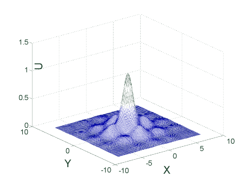
Figure 1: Solution of Eq. (3.19) with $V_{0}=3$ and $\mu=3.7$.

with $A=1$ and $W=1$. We take the free parameter $\Delta\tau=1$ and compute $c$ and $\gamma$ until the solution reaches the accuracy of $10^{-3}$ (see Remark 3.5). The latest computed values are $c=1.20$ and $\gamma=3.71$. Then the iterations are continued until the solution reaches the accuracy of $10^{-10}$. The final solution is shown in Fig. 1, and a short Matlab code that can be used to obtain it is given in Appendix 1.

The total number of iterations taken by the generalized Petviashvili method is about 180. (Here and below we quote the number of iterations rounded to the nearest ten. The reason is that this number may slightly depend on the size of the computational domain and possibly other technical factors.) For comparison, the optimally accelerated ITEM (with the corresponding power of the solitary wave being $P=3.0$) reaches the same solution in about 300 iterations; see Example 9.1 in [4]. The modification of the ITEM where one seeks a solitary wave with a specified peak amplitude [4] rather than the power converges to the same solution in 130 iterations. The ad hoc modification of the original Petviashvili method, proposed for Eq. (3.19) in [9], takes about 420 iterations to converge to the same accuracy [4]. It should be noted that the value $\Delta\tau=1$, which we used in this Example, does not lead to the fastest convergence of algorithm (3.6)–(3.8). For instance, we found that for $\Delta\tau=1.3$, the convergence rate of our method is nearly the fastest, and the method converges in about 140 iterations. The dependence of the convergence rate on the step size $\Delta t$ is discussed in the companion paper [13].

Example 3.2  In this Example we present a case where two modifications of the original Petviashvili method proposed in Refs. [9] and [12] diverge, but the generalized Petviashvili method, proposed in this Section, converges. We seek an anti-symmetric solution of the following equation with a double-well potential:

$$u_{xx}+V(x)u-u^{3}=\mu u,\qquad V(x)=6\left({\rm sech}^{2}(x-1)+{\rm sech}^{2}(x+1)\right)$$ (3.21)

for $\mu=1.43$. (The solution with this value of the propagation constant has the power $P\equiv\int_{-\infty}^{\infty}u^{2}\,dx=10$ and was originally found in [4] by the ITEM.) As the initial condition, we take

$$u_{0}=2x\,e^{-x^{2}}+\epsilon\,e^{-x^{2}},$$ (3.22)

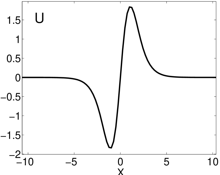
Figure 2: Anti-symmetric solutions of Eq. (3.21) with $\mu=1.43$.

with $\epsilon$ being either zero or $0.001$. As in Example 3.1, we compute $c$ and $\gamma$ only as long as the error exceeds $10^{-3}$; then we use these latest computed values for the rest of the iterations. We first set $\epsilon=0$ in (3.22) and empirically find that $\Delta\tau=1.6$ results in the fastest convergence (in about 40 iterations) of the generalized Petviashvili method (3.6)–(3.8); the iteratively computed parameters of the algorithm are in this case: $c=5.04$ and $\gamma=0.21$. The corresponding solution is shown in Fig. 2. Next, when we introduce a small symmetric component into the initial condition (3.22) by setting $\epsilon=0.001$, the iterations still converge to that solution, although at a lower rate (in about 170 iterations).

We now apply to Eq. (3.21) the modifications of the original Petviashvili method proposed in Refs. [9] and [12]. The former of these methods has the form:

$$u_{n+1}=M^{-1}\left(C_{n}^{\gamma_{\rm lin}}V(x)u_{n}-C_{n}^{\gamma_{\rm nl}}u_{n}^{3}\right),$$ (3.23)

where $M=\mu-\partial_{x}^{2}$ and the factor $C_{n}$ is chosen so that it equals one when $u_{n}$ is an exact solution of (3.21):

$$C_{n}=\frac{\langle u_{n},\,(-M+V(x))u_{n}\rangle}{\langle u_{n},\,u_{n}^{3}\rangle}.$$ (3.24)

The constants $\gamma_{\rm lin}$ and $\gamma_{\rm nl}$ in (3.23) are to be chosen empirically; in [9], the choice $\gamma_{\rm lin}=0.5$ and $\gamma_{\rm nl}=1.5$ was suggested. The method of Ref. [12] for Eq. (3.21) can be shown to reduce to the same form (3.23), where now

$$C_{n}=\frac{\langle u_{n},\,(-1+M^{-1}V(x))u_{n}\rangle}{\langle u_{n},\,M^{-1}u_{n}^{3}\rangle}$$ (3.25)

and $\gamma_{\rm lin}=0.5$ and $\gamma_{\rm nl}=1.5$. (Unlike in the ad hoc method of Ref. [9] where these values of $\gamma_{\rm lin}$ and $\gamma_{\rm nl}$ were “guessed”, in the method of Ref. [12] these values can be derived from Eqs. (5) and (6) of that paper.) For the solution of (3.21) with $\mu=1.43$, both these methods converged in about 20 iterations when started at the initial condition (3.22) with $\epsilon=0$. However, they both diverged for $\epsilon=0.001$, in contrast to our generalized Petviashvili method, which converged for either value of $\epsilon$.

Example 3.3  In this Example, we show that the calculations of Sections 2 and 3 for the optimal value of $\gamma$ can be carried out even when the nonlinearity of the equation is nonlocal. Consider a stationary wave equation

$$\left(1-\frac{1}{2}\nabla^{2}\right)u\,=\,u\,\nabla^{-2}\left(\frac{\partial^{2}}{\partial x^{2}}u^{2}\right).$$ (3.26)

This equation, which has a nonlocal operator $\nabla^{-2}$ on the right hand side, can be rewritten as a system of two local equations:

$$\begin{array}[]{l}\displaystyle\left(1-\frac{1}{2}\nabla^{2}\right)u\,=\,u\,v,\vspace{0.1cm}\\ \displaystyle\nabla^{2}v=\frac{\partial^{2}}{\partial x^{2}}u^{2}\,.\end{array}$$ (3.27)

This system arises as the small-field approximation in the theory of light propagation in photorefractive media; see, e.g., [14]. Let us note that Eqs. (3.27) cannot be handled by the method described in Section 4 below because the corresponding linearized operator is not self-adjoint. However, the original nonlocal Eq. (3.26) can be handled by the method of Sections 2 and 3. To that end, let us linearize this equation near the exact solution $u$:

$$L\tilde{u}\equiv-\left(1-\frac{1}{2}\nabla^{2}\right)\tilde{u}+\tilde{u}\,\nabla^{-2}\left(\frac{\partial^{2}}{\partial x^{2}}u^{2}\right)+u\nabla^{-2}\left(\frac{\partial^{2}}{\partial x^{2}}2u\tilde{u}\right).$$ (3.28)

Then, using (3.26),

$$Lu\,=\,2u\nabla^{-2}\left(\frac{\partial^{2}}{\partial x^{2}}u^{2}\right)\,=\,2\left(1-\frac{1}{2}\nabla^{2}\right)u\,.$$ (3.29)

This is Eq. (2.13) with $p=3$ and $M=\left(1-\frac{1}{2}\nabla^{2}\right)$; hence, from (1.10), $\gamma_{\rm opt}=3/2$. It is this value of $\gamma$ which the authors of [14] used (without justification) in the original Petviashvili algorithm applied to system (3.27).

4 Generalization of the Petviashvili method for coupled nonlinear wave equations

Here we will first show how the generalized Petviashvili method of Section 3 can be extended to obtain solitary waves in Hamiltonian systems of coupled nonlinear equations. Then we will present the corresponding examples. To make the essential details of our technique clearer, we will focus on the case of two coupled equations, while commenting on the extension to three and more equations in Appendix 3.

4.1 Derivation of the generalized Petviashvili method for coupled equations

Consider the following system of equations for the real-valued components $u$ and $v$ of the solitary wave:

$$-\left(\begin{array}[]{cc}M_{11}&0\\ 0&M_{22}\end{array}\right)\left(\begin{array}[]{c}u\\ v\end{array}\right)+\left(\begin{array}[]{c}F_{1}({\bf x},u,v)\\ F_{2}({\bf x},u,v)\end{array}\right)\;\equiv\;{\bf L}_{0}\left(\begin{array}[]{c}u\\ v\end{array}\right)\;=\;\left(\begin{array}[]{c}0\\ 0\end{array}\right)\,,\qquad\lim_{|{\bf x}|\rightarrow\infty}\left(\begin{array}[]{c}u\\ v\end{array}\right)=\left(\begin{array}[]{c}0\\ 0\end{array}\right),$$ (4.1)

where $M_{11}$ and $M_{22}$ are self-adjoint positive definite operators. (Whenever symmetric (see below) off-diagonal terms $M_{12}v$ and $M_{12}u$ are present in the first and second equations, they can always be removed by a linear transformation.) The restrictions on functions $F_{1,2}$ become clear when one considers the linearized operator, ${\bf L}$, of Eq. (4.1):

$${\bf L}\left(\begin{array}[]{c}\tilde{u}\\ \tilde{v}\end{array}\right)=\left(\begin{array}[]{cc}-M_{11}+F_{1,u}&F_{1,v}\\ F_{2,u}&-M_{22}+F_{2,v}\end{array}\right)\left(\begin{array}[]{c}\tilde{u}\\ \tilde{v}\end{array}\right)\,,$$ (4.2)

where $F_{1,u}\equiv\partial F_{1}/\partial u$, etc. Recall that the linearized operator $L$ played the key role in the analysis of Section 2; in particular, it was crucial for the derivation of Eqs. (2.15)–(2.17) and the discusion following Eq. (2.19) that $L$ was self-adjoint. Similarly, to carry out that analysis for the coupled Eqs. (4.1), we require that ${\bf L}$ in (4.2) be self-adjoint. This yields the condition

$$F_{1,v}=F_{2,u}\,.$$ (4.3)

Thus, our method will be applicable to systems of form (4.1) where $F_{1}$ and $F_{2}$ satisfy condition (4.3). Note that these functions may contain nonlocal operators as in Example 3.3 above.

Our plan now is as follows. We will first present a generalization of the linearized continuous flow (2.8), then will comment on it, and, finally, will state the vector counterpart of the “delinearized” algorithm (3.6). The extension of (2.8) to the vector case is:

$$\left(\begin{array}[]{c}\tilde{u}\\ \tilde{v}\end{array}\right)_{\tau}={\bf N}^{-1}{\bf L}\left(\begin{array}[]{c}\tilde{u}\\ \tilde{v}\end{array}\right)-\sum_{k=1}^{2}\gamma_{k}\frac{\left\langle\vec{\bf e}_{k},\,{\bf L}\left(\begin{array}[]{c}\tilde{u}\\ \tilde{v}\end{array}\right)\right\rangle}{\langle\vec{\bf e}_{k},\,{\bf N}\vec{\bf e}_{k}\rangle}\,\vec{\bf e}_{k}\,,$$ (4.4)

$$\gamma_{k}=1+\frac{1}{\alpha_{k}\Delta\tau}\,,\qquad\alpha_{k}=\frac{\langle\vec{\bf e}_{k},\,{\bf L}\vec{\bf e}_{k}\rangle}{\langle\vec{\bf e}_{k},\,{\bf N}\vec{\bf e}_{k}\rangle}\,,\qquad k=1,2,$$ (4.5)

where ${\bf N}$ is a self-adjoint, positive definite matrix operator, whose form will be discussed shortly, and $\vec{\bf e}_{k}$ and $\alpha_{k}$ are the approximate eigenvectors and eigenvalues of ${\bf N}^{-1}{\bf L}$:

$${\bf L}\,\vec{\bf e}_{k}\,\approx\,\alpha_{k}{\bf N}\,\vec{\bf e}_{k}\,.$$ (4.6)

The analysis of convergence of Eq. (4.4) proceeds along the lines of the corresponding analysis in Section 2 with one minor modification: In the derivation of Eq. (4.5) for $\gamma_{k}$, one needs to use the (approximate) orthogonality of $\vec{\bf e}_{1}$ and $\vec{\bf e}_{2}$:

$$\langle\vec{\bf e}_{1},\,{\bf N}\vec{\bf e}_{2}\rangle=0\,.$$ (4.7)

Condition (4.7) follows from (4.6) and the fact that both ${\bf L}$ and ${\bf N}$ are self-adjoint.

Now we discuss the computationally efficient choice of operator ${\bf N}$ and vectors $\vec{\bf e}_{k}$. It is this choice that makes the generalization of the method of Section 3 to the case of coupled equations nontrivial; hence it constitutes an important technical result of this Section. For the simplicity of presentation, we assume that both $M_{11}$ and $M_{22}$ in (4.2) have form (1.5), with possibly different $\mu$’s. (The extension to a more general form of these operators is straightforward and one instance of it is given in Example 4.3 below.) Then, the form of ${\bf N}$ that we advocate, and which we used in all of the examples presented in Section 4.2, is

$${\bf N}=\left(\begin{array}[]{cc}N_{1}&0\\ 0&N_{2}\end{array}\right),\qquad N_{k}=c_{k}-b_{k}\nabla^{2},\quad k=1,2.$$ (4.8)

One may wonder if the more general form that includes (symmetric) off-diagonal terms $c_{12}-b_{12}\nabla^{2}$ would result in a more efficient method. The answer, based on our experimentation with both this more general form and the simpler form (4.8), is negative. First, the coding of the part of the computer program that would calculate all of the coefficients $c_{k}$, $b_{k}$, and $c_{12}$, $b_{12}$ for the more general form of $N$ is considerably more tedious than the corresponding coding for the simpler form (4.8). This part of the program would be difficult to debug had a mistake in it occurred. Moreover, the simplicity of the original Petviashvili method, which is one of its main advantages over the Newton’s method, would be compromised by this coding issue. Second, in our simulations we also found that, in some cases, unless the initial condition $(u_{0},v_{0})$ is “very” close to the exact solitary wave $(u,v)$, then the ${\bf N}$ calculated as a full matrix may turn out not to be positive definite, which would result in the divergence of the iterations. On the other hand, we verified that the simpler, diagonal form (4.8) does not have either of the above drawbacks.

Let us now show how $c_{1,2}$ and $b_{1,2}$ in (4.8) can be computed while assuming a general form of the eigenvector $\vec{\bf e}_{1}$, and then will argue that one can and should take $\vec{\bf e}_{1}=(u,v)^{T}$. Let

$${\bf L}\equiv\left(\begin{array}[]{cc}L_{11}&L_{12}\\ L_{12}&L_{22}\end{array}\right),\qquad\vec{\bf e}_{1}\equiv\left(\begin{array}[]{c}e_{11}\\ e_{21}\end{array}\right),$$ (4.9)

where each of $L_{ij}$ is a self-adjoint operator. As in Section 3, we require that

$$\frac{\langle{\bf N}\vec{\bf e}_{1},\,{\bf L}\vec{\bf e}_{1}\rangle^{2}}{\langle{\bf N}\vec{\bf e}_{1},\,{\bf N}\vec{\bf e}_{1}\rangle\langle{\bf L}\vec{\bf e}_{1},\,{\bf L}\vec{\bf e}_{1}\rangle}\,=\,\max$$ (4.10)

and then find the equations for $c_{1,2}$ and $b_{1,2}$ by setting the derivatives of the l.h.s. with respect to these parameters to zero. Thus, similarly to (3.10), one obtains a system of four equations:

$$\frac{\langle{\bf N}_{r}\vec{\bf e}_{1},\,{\bf L}\vec{\bf e}_{1}\rangle}{\langle{\bf N}_{r}\vec{\bf e}_{1},\,{\bf N}\vec{\bf e}_{1}\rangle}\,=\,\frac{\langle{\bf N}\vec{\bf e}_{1},\,{\bf L}\vec{\bf e}_{1}\rangle}{\langle{\bf N}\vec{\bf e}_{1},\,{\bf N}\vec{\bf e}_{1}\rangle},$$ (4.11)

$${\bf N}_{r}\equiv\frac{\partial{\bf N}}{\partial r},\qquad r=\{c_{1},c_{2},b_{1},b_{2}\}\,.$$

Since the r.h.s. of all these equations is the same, one can obtain a system of three equations for the four unknown parameters $r$ by setting the correponding l.h.s.’s equal to each other. It is easy to see, by inspection, that this system is linear and homogeneous, and hence it produces a solution for $\{c_{1},c_{2},b_{1},b_{2}\}$ that is unique up to multiplication by an arbitrary constant. (Such an arbitrariness is expected because operator ${\bf N}$ is defined by (4.6) only up to an arbitrary factor.) Next, any one of Eqs. (4.11) can be taken as the remaining fourth equation for $\{c_{1},c_{2},b_{1},b_{2}\}$. We verified that such an equation is satisfied identically for the solution $\{c_{1},c_{2},b_{1},b_{2}\}$ determined from the aforementioned linear homogeneous system of three equations.

The solution of that system can most easily be found as follows. Equating the l.h.s.’s of Eqs. (4.11) with $r=c_{k}$ to those with the corresponding $r=b_{k}$ yields:

$$\kappa_{k}\equiv\frac{c_{k}}{b_{k}}=\frac{\left\langle\left(\,\langle\nabla^{2}e_{k1},\,\sum_{j=1}^{2}L_{kj}e_{j1}\rangle\,e_{k1}-\langle e_{k1},\,\sum_{j=1}^{2}L_{kj}e_{j1}\rangle\,\nabla^{2}e_{k1}\right),\,\nabla^{2}e_{k1}\right\rangle}{\left\langle\left(\,\langle\nabla^{2}e_{k1},\,\sum_{j=1}^{2}L_{kj}e_{j1}\rangle\,e_{k1}-\langle e_{k1},\,\sum_{j=1}^{2}L_{kj}e_{j1}\rangle\,\nabla^{2}e_{k1}\right),\,e_{k1}\right\rangle}\,,\qquad k=1,2.$$ (4.12)

Then, equating the l.h.s.’s of (4.11) with $r=c_{1}$ and $r=c_{2}$ yields

$$\frac{b_{2}}{b_{1}}=\frac{\langle e_{11},\,(\kappa_{1}-\nabla^{2})e_{11}\rangle\;\langle e_{21},\,\sum_{j=1}^{2}L_{2j}e_{j1}\rangle}{\langle e_{21},\,(\kappa_{2}-\nabla^{2})e_{21}\rangle\;\langle e_{11},\,\sum_{j=1}^{2}L_{1j}e_{j1}\rangle}\,.$$ (4.13)

The pseudocode for the time-efficient computation (i.e., a computation that avoids repeated evaluation of the same quantities) is presented in Appendix 2. As in Remark 3.5, we note that $c_{1,2},\;b_{1,2}$ and the corresponding values of $\alpha_{1,2}$ and $\gamma_{1,2}$ need only be computed up to the moment when the iterations approach the exact solution with some relatively low accuracy (say, $10^{-3}$). The remaining iterations, up to a higher accuracy, can be carried out with those latest computed values of these parameters.

Remark 4.1  Let us reiterate that the above algorithm of finding the coefficients of operator ${\bf N}$, which can be straightforwardly generalized to any number of coupled equations (see Appendix 3), is one of the main results of this Section. The key part here is that a unique set of these coefficients can always (except, maybe, in some pathological cases which we never encountered) be found by solving a linear system of equations.

We now discuss the choice of the eigenvectors $\vec{\bf e}_{1}$ and $\vec{\bf e}_{2}$. First, we note that since these eigenvectors enter Eq. (4.4) on equal footing, it might seem that it would be “more correct” to replace the l.h.s. of (4.10) by

$$\sum_{k=1}^{2}\frac{\langle{\bf N}\vec{\bf e}_{k},\,{\bf L}\vec{\bf e}_{k}\rangle^{2}}{\langle{\bf N}\vec{\bf e}_{k},\,{\bf N}\vec{\bf e}_{k}\rangle\langle{\bf L}\vec{\bf e}_{k},\,{\bf L}\vec{\bf e}_{k}\rangle}\,.$$ (4.14)

However, this is not so because, in particular, the corresponding counterpart of (4.11) becomes a truly nonlinear system for $\{c_{1},c_{2},b_{1},b_{2}\}$ and hence cannot be easily solved. Therefore, we continue to use the results obtained from (4.10). Next, a reasonable, although not the most general, choice for $\vec{\bf e}_{1}$ is

$$\vec{\bf e}_{1}=\left(\begin{array}[]{r}u\\ \rho_{21}v\end{array}\right)\,.$$ (4.15)

Then $\vec{\bf e}_{2}$ is sought in the form

$$\vec{\bf e}_{2}=\left(\begin{array}[]{r}\rho_{12}u\\ v\end{array}\right)\,,$$ (4.16)

where $\rho_{12}$ is determined from the orthogonality condition (4.7):

$$\rho_{12}=-\rho_{21}\,\frac{\langle v,\,N_{2}v\rangle}{\langle u,\,N_{1}u\rangle},$$ (4.17)

where $N_{1}$ and $N_{2}$ are found from (4.8), (4.12), and (4.13) for each given value of $\rho_{21}$.

The issue is then to determine coefficient $\rho_{21}$. This can be done by imposing the requirement that quantity (4.14), which is a nonlinear function of $\rho_{21}$, be maximized with respect to that coefficient. It can be shown, with some effort, that this nonlinear optimization problem can be solved time-efficiently, i.e. without repeated evaluation of the inner products in (4.14). We performed several experiments with the Examples reported in Section 4.2 and concluded that simply taking

$$\rho_{21}=1$$ (4.18)

instead of solving the optimization problem for that coefficient was the optimal choice, for the following reasons. In many cases, we empirically found that the “optimal” value for $\rho_{21}$ was close to one, and hence the considerable complexification of the code needed to compute that value did not justify the obtained improvement of the convergence rate by just a few percent. Moreover, in some examples we found that the iterations were initially selecting a value of $\rho_{21}$ that was not close to (4.18), and then they would quickly diverge. (This probably occurred when the initial condition was not sufficiently close to the exact solution.) On the other hand, setting $\rho_{21}$ according to (4.18) always resulted in the convergence of the iterations. Thus we conclude that taking the eigenvectors $\vec{\bf e}_{1,2}$ according to Eqs. (4.15)–(4.18) constitutes the optimal practical choice. The results presented in Section 4.2 justify the validity of this choice.

We now state the algorithm of the generalized Petviashvili method for coupled nonlinear wave equations, which is obtained by “delinearizing” Eq. (4.4):

$$\left(\begin{array}[]{c}u\\ v\end{array}\right)_{n+1}=\left(\begin{array}[]{c}u\\ v\end{array}\right)_{n}+\left[{\bf N}^{-1}\left({\bf L}_{0}\left(\begin{array}[]{c}u\\ v\end{array}\right)\,\right)_{n}-\sum_{k=1}^{2}\gamma_{k}\frac{\left\langle\vec{\bf e}_{k,n},\,\left({\bf L}_{0}\left(\begin{array}[]{c}u\\ v\end{array}\right)\,\right)_{n}\right\rangle}{\langle\vec{\bf e}_{k,n},\,{\bf N}\vec{\bf e}_{k,n}\rangle}\,\vec{\bf e}_{k,n}\,\right]\Delta\tau\,,$$ (4.19)

where $\vec{\bf e}_{k,n}$ are computed using the components $u_{n},v_{n}$ at each iteration, and ${\bf N}$ and $\gamma_{k}$ are computed iteratively until the solution reaches a prescribed accuracy (see Remark 3.5). Iteration scheme (4.19) along with the details of calculation of $N$ and $\vec{\bf e}_{k}$ (Eqs. (4.8), (4.12), (4.13), and (4.15)–(4.18)) is the main result of this Section. As we noted in the Introduction, the reader who is not interested in implementation issues of this algorithm may skip the remainder of this Section.

Remark 4.2  This Remark extends to the case of coupled equations the observation stated in Remark 3.2. Namely, to calculate the coefficients of ${\bf N}$ and the eigenvalues $\alpha_{1,2}$ at the $(n+1)$st iteration, one requires the values of ${\bf L}\vec{\bf e}_{1,2}$, where $\vec{\bf e}_{1,2}$ are found from (4.15) and (4.16) using the available values of $u_{n}$ and $v_{n}$. Now, the expressions

$${\bf L}\vec{\bf e}_{k}+{\rm const}\cdot{\bf L}_{0}\left(\begin{array}[]{c}u_{n}\\ v_{n}\end{array}\right)$$ (4.20)

are equal to each other up to the order $O(\tilde{u}_{n},\tilde{v}_{n})$ for any value of the constant, and so the issue is which of these expressions to use when computing ${\bf L}\vec{\bf e}_{1,2}$. In our simulations, we found that computing ${\bf L}\vec{\bf e}_{k}$ at the $n$th iteration as

$${\bf L}\vec{\bf e}_{k}\,\equiv\,({\bf L}\vec{\bf e}_{k})_{n}-\left({\bf L}_{0}\left(\begin{array}[]{c}u\\ v\end{array}\right)\,\right)_{n},\qquad k=1,2$$ (4.21)

(i.e. taking in (4.20)  const=$-1$) results in a sufficiently broad range of initial conditions $(u_{0},v_{0})$ that converge to the solitary wave $(u,v)$. For comparison, taking in (4.20) const=$0$ required the initial conditions to be much closer to the exact solution for the iterations to converge. Thus, to compute $\alpha_{1,2}$ in (4.5), we used the expression given by (4.21). Note that while for $k=1$, this result is an obvious extension of (3.14) (upon taking into account (4.15) and (4.18)), for $k=2$ this result is not obvious and was arrived at upon experimentation with various values of the constant in (4.20).

Remark 4.3  When system (4.1) is decoupled, i.e., $F_{1,v}=F_{2,u}=0$, the approximate eigenvalues $\alpha_{1,2}$ of ${\bf N}^{-1}{\bf L}$ must be equal. Indeed, in this case, from (4.5) one has:

$$\begin{array}[]{rl}\alpha_{1}=&\displaystyle\frac{\langle u,\,L_{11}u\rangle}{\langle u,\,N_{1}u\rangle}\cdot\frac{1+(\langle v,\,L_{22}v\rangle/\langle u,\,L_{11}u\rangle)}{1+(\langle v,\,N_{2}v\rangle/\langle u,\,N_{1}u\rangle)}\,,\vspace{0.2cm}\\ \alpha_{2}=&\displaystyle\frac{\langle u,\,L_{11}u\rangle}{\langle u,\,N_{1}u\rangle}\cdot\frac{\rho_{12}^{2}+(\langle v,\,L_{22}v\rangle/\langle u,\,L_{11}u\rangle)}{\rho_{12}^{2}+(\langle v,\,N_{2}v\rangle/\langle u,\,N_{1}u\rangle)}\,.\end{array}$$ (4.22)

Next, using Eq. (4.13) with $L_{12}\equiv L_{21}=0$, one obtains:

$$\frac{\langle v,\,N_{2}v\rangle}{\langle u,\,N_{1}u\rangle}\,=\,\frac{b_{2}}{b_{1}}\,\frac{\langle v,\,(\kappa_{2}-\nabla^{2})v\rangle}{\langle u,\,(\kappa_{2}-\nabla^{2})u\rangle}\,=\,\frac{\langle v,\,L_{22}v\rangle}{\langle u,\,L_{11}u\rangle}\,.$$ (4.23)

Substituting (4.23) into (4.22), one obtains $\alpha_{1}=\alpha_{2}$. This fact is, thus, a consequence of the coefficients of the entries of ${\bf N}$ satisfying (4.13).

Remark 4.4  For completeness of this presentation, we note that it is possible to find such a form of Eqs. (4.1) for which the coefficients of operator ${\bf N}$, the coefficient $\rho_{12}$, and the eigenvalues $\alpha_{1,2}$ (and hence $\gamma_{1,2}$) can be obtained analytically (i.e., similarly to how the optimal $\gamma$ given by (2.18) is obtained for Eq. (1.1)). For the case of two coupled equations, we derive the corresponding class of equations in Appendix 4. A particular equation from that class is considered in Example 4.3 below. Note that for this class of equations, ${\bf N}={\rm diag}(M_{11},M_{22})$, where $M_{11}$ and $M_{22}$ are defined in Eq. (4.1). This is a counterpart of the relation $N=M$ for a single equation with power-law nonlinearity, noted after Eq. (3.11).

4.2 Examples of application of the generalized Petviashvili method to coupled equations

The examples presented below are restricted to systems of two coupled stationary wave equations. We focused on those examples where the components $u$ and $v$ of the solitary wave have distinctly different amplitudes and widths; this is done to apply as strict as possible a test to our method. Also, in all of these examples except Example 4.1, the computational domain was a square with the side of $8\pi$ and $2^{7}$ mesh points along each side. In Example 4.1, the side of the square was $12\pi$ with $2^{8}$ mesh points per side.

Example 4.1  Consider a vector generalization of the equation from Example 3.1:

$$\begin{array}[]{l}\nabla^{2}u+4(\cos^{2}x+\cos^{2}y)u+u(u^{2}+\sigma v^{2})\,=\,\mu_{1}u\vspace{0.1cm}\\ \nabla^{2}v+4(\cos^{2}x+\cos^{2}y)v+v(\sigma u^{2}+4v^{2})\,=\,\mu_{2}v.\end{array}$$ (4.24)

Here the asymmetry between $u$ and $v$ is provided by two sources:  (i) by the different coefficients, ‘$1$’ and ‘$4$’, in front of the self-nonlinearity terms and, more importantly,  (ii) by the different propagation constants $\mu_{1}$ and $\mu_{2}$. Specifically, we used

$$\mu_{1}=4.95\quad{\rm and}\quad\mu_{2}=6.5.$$

In the absence of coupling ($\sigma=0$), this corresponds to the solution $u$ being near the edge of the zeroth band gap and $v$ being suficiently far away from that edge. Consequently, $v$ is significantly “taller” and more localized than $u$ (see, e.g., [15]). When the coupling is present ($\sigma>0$), the structure of the composite solution remains qualitatively the same; such a solution for

$$\sigma=0.5$$ (4.25)

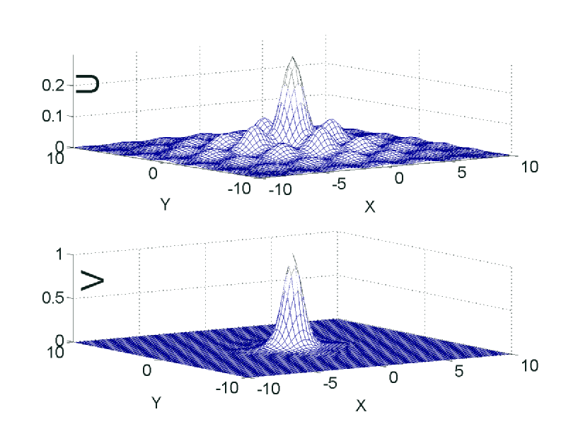
Figure 3: Solution of Eqs. (4.24) with $\mu_{1}=4.95$, $\mu_{2}=6.5$, and $\sigma=0.5$. Note the different vertical scales of the $u$- and $v$-components.

is plotted in Fig. 3. Starting with the initial condition

$$\begin{array}[]{l}\displaystyle u_{0}=A_{1}\,e^{-(x^{2}+y^{2})/W_{1}^{2}}\vspace{0.1cm}\\ \displaystyle v_{0}=A_{2}\,e^{-(x^{2}+y^{2})/W_{2}^{2}},\end{array}$$ (4.26)

where $A_{1,2}$ and $W_{1,2}$ are listed in Table 1, the iterations (4.19) with $\Delta\tau=1$ takes about 710 iterations to converge to accuracy of $10^{-10}$. Here and below, the accuracy for two-component solitary waves is defined similarly to (1.11):

$$E_{n}=\left(\frac{\langle u_{n}-u_{n-1},u_{n}-u_{n-1}\rangle}{\langle u_{n},u_{n}\rangle}+\frac{\langle v_{n}-v_{n-1},v_{n}-v_{n-1}\rangle}{\langle v_{n},v_{n}\rangle}\right)^{1/2}\,.$$ (4.27)

In all of the examples of this Section, we monitored the following quantities: coefficient $\rho_{12}$ (see (4.16)–(4.18)); factors

$$I_{k}=\frac{\langle{\bf N}\vec{\bf e}_{k},\,{\bf L}\vec{\bf e}_{k}\rangle^{2}}{\langle{\bf N}\vec{\bf e}_{k},\,{\bf N}\vec{\bf e}_{k}\rangle\langle{\bf L}\vec{\bf e}_{k},\,{\bf L}\vec{\bf e}_{k}\rangle},\qquad k=1,2,$$ (4.28)

which show how close vectors $\vec{\bf e}_{k}$ are to the true eigenvectors of  ${\bf N}^{-1}{\bf L}$; the eigenvalues $\alpha_{1,2}$ (see (4.6)); and the coefficients $c_{1},c_{2},b_{2}$ of ${\bf N}$ (we set $b_{1}=1$ without loss of generality). These quantities are reported in Table 1. In particular, one sees that $\vec{\bf e}_{1}$ is a closer approximation to its corresponding true eigenvector of ${\bf N}^{-1}{\bf L}$ than $\vec{\bf e}_{2}$ is to its true eigenvector; this is expected since the coefficients of operator ${\bf N}$ are computed using $\vec{\bf e}_{1}$. Note, however, from the reported values of $I_{1,2}$, that both $\vec{\bf e}_{1}$ and $\vec{\bf e}_{2}$ approximate their respective true eigenvectors quite well.

To benchmark the performance of the method, we also obtained the solution of the uncoupled system, (4.24) with $\sigma=0$, in two ways. First, we used the vector generalization of the Petviashvili method described in Section 4.1. For $\Delta\tau=1$, the iterations converged to accuracy $10^{-10}$ in about 950 iterations. (Let us note, in passing, that the numerically found $\alpha_{1,2}$ agree with Remark 4.6.) As the second way of obtaining the same solutions, we solved each of the uncoupled equations (4.24) using the generalized Petviashvili method for a single equation, as described in Section 3.1. The iterations for components $u$ and $v$ took, respectively, about 950 and 80 iterations to converge to the accuracy of $10^{-10}$. Comparing this with the number of iterations needed to obtain the solution of the uncoupled system via the first method, we conclude that the convergence rate of the vector form of the generalized Petviashvili method is determined by such a rate for the more slowly converging component of the solitary wave.

Example 4.2  We now consider a system of linearly coupled nonlinear Schrödinger equations:

$$\begin{array}[]{l}\nabla^{2}u+u^{3}+\sigma v=u\vspace{0.1cm}\\ \nabla^{2}v+v^{3}+\sigma u=v\,.\end{array}$$ (4.29)

This system extends to two dimensions the equations of the so-called nonlinear directional coupler [16]. In one spatial dimension, these equations are known to possess symmetric ($u=v$), anti-symmetric ($u=-v$), and, for $\sigma<0.6$, asymmetric ($|u|\neq|v|$) solitary waves [16]. The smaller the $\sigma$, the greater the asymmetry between the two components of the latter solution. To our knowledge, asymmetric solutions of the two-dimensional system (4.29) have not been reported previously.

We considered Eqs. (4.29) with $\sigma=0.5$. By trial and error, we found that the initial condition (4.26) with the parameters reported in Table 1 leads the iterations to converge to the solution depicted in Fig. 4. (It should be noted that this initial condition must be quite close to the exact solution in order for the iterations to converge. For example, if one takes $A_{2}=0.4$ or $A_{2}=0.6$ instead of $0.5$, as in Table 1, then the iterations converge to either the symmetric or anti-symmetric solitary wave.) Next, by running the simulations and monitoring, at each iteration, the approximate eigenvalues $\alpha_{1,2}$, we observed that $\alpha_{2}$ is a large negative number (see Table 1). Then, to satisfy the necessary convergence condition (2.24), one needs to use a rather small step size $\Delta\tau$. By trial and error, we found that $\Delta\tau=0.08$ results in nearly the fastest convergence of the method for system (4.29).

Note that since $\alpha_{2}<0$ in this example, the iterations would still converge if $\gamma_{2}$ were set to zero.

Example 4.3  As the last example, we applied method (A3.2) to a system of equations that describe copropagation of the fundamental and second harmonic fields in an optical medium with quadratic nonlinearity:

$$\begin{array}[]{l}\displaystyle\nabla^{2}u+uv=\mu_{1}u\vspace{0.1cm}\\ \displaystyle\nabla^{2}_{\delta}v+\frac{1}{2}u^{2}=\mu_{2}v,\qquad\nabla^{2}_{\delta}\equiv\partial^{2}_{x}+\delta\partial^{2}_{y}\,.\end{array}$$ (4.30)

Multidimensional solutions of this and related systems were considered in quite a few studies; see, e.g., a recent paper [17] and references therein. It should be noted that Eqs. (4.30) are a special case of the system of two coupled wave equations for which all the coefficients in the Petviashvili method can be determined analytically (see Eq. (A4.14) in Appendix 4). In particular, as follows from the last paragraph of Appendix 4, one should have $c_{1,2}=\mu_{1,2}$ and $b_{2}=1$. Thus, this example provides a test of whether our method would obtain these coefficients correctly, and it indeed did so. Specifically, we took

$$\delta=10,\quad\mu_{1}=1.5,\quad\mu_{2}=9;$$ (4.31)

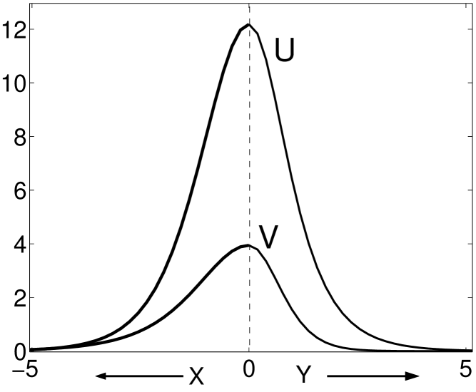
Figure 5: Solution of Eqs. (4.30), (4.31) along the $x$-axis (to the left of the dashed line) and the $y$-axis (to the right of the dashed line).

then one can see that the values of $c_{1,2}$ and $b_{2}$, reported in Table 1, are indeed as stated above. Moreover, the values of $\rho_{12}$ and $\alpha_{1,2}$ agree with those given by Eq. (A4.12) in Appendix 4. Finally, we note that the formulae for the calculation of $c_{1,2}$, $b_{2}$, $\rho_{12}$, and $\alpha_{1,2}$ are those given in Section 4.1 with one modification: all occurrences of $\nabla^{2}v$ should be replaced with $\nabla^{2}_{\delta}v$. The corresponding solitary wave is shown in Fig. 5.

5 Summary

In this work, we obtained the following two main results.

First, in Section 3, we extended the well-known Petviashvili iteration method to find solitary wave solutions of a broad class of Hamiltonian nonlinear wave equations with arbitrary form of nonlinearity and potential function; see Eq. (3.1). Our algorithm is given by Eqs. (3.6)–(3.8), (3.11), and (3.12). The generalized Petviashvili method can be applied even when the equation is nonlocal; see Example 3.3. The computational cost of this method only slightly exceeds that of the original Petviashvili method, since the (few) parameters required to carry out the iterations need to be computed only until the solution reaches some relatively low accuracy; see Remark 3.5.

Second, in Section 4, we extended this method to systems of coupled Hamiltonian wave equations. Our main result here was the finding of a way in which all the required parameters of the iteration scheme can be computed by explicit expressions, obtained from solving a simple linear system of algebraic equations. The algorithm (for two equations) is given by Eqs. (4.19), (4.8), (4.12), (4.13), and (4.15)–(4.18)).

Appendices 1 and 2 contain, respectively, a Matlab code illustrating the algorithm of Section 3 and a pseudocode for the algorithm of Section 4. Appendix 3 contains an extension of the algorithm of Section 4 to three (and more) equations. Finally, Appendix 4 contains a collateral result: the form of a system of two coupled equations for which the parameters of our generalized Petviashvili iteration scheme can be found analytically (as in the original Petviashvili method for a single equation with power-law nonlinearity).

Appendix 1:  Matlab code for Example 3.1

N=2^7;  d=10*pi/N;                    % mesh sizes along x and y
x=[-5*pi:d:5*pi-d]; y=x;
[X,Y]=meshgrid(x,y);                  % 2D x- and y-arrays
kx=2*pi/(10*pi)*[0:N/2-1  -N/2:-1];  ky=kx;
[KX,KY]=meshgrid(kx,ky);   K2=KX.^2+KY.^2;
Dt=0.4;                               % Delta tau
mu=3.7;                               % prop. constant of the soliton
W=3*((cos(X)).^2+(cos(Y)).^2)-mu;     % V(x)-mu
u0=1.5*exp(-(X.^2+Y.^2));  u=u0;      % initial condition
norm_Du=1;                            % initialize E_n defined in (1.11)
while norm_Du >= 10^(-10)
    u_old=u;   fftu=fft2(u);   ucube=u.^3;   DEL_u=real(-ifft2(K2.*fftu));
    if norm_Du >= 10^(-3)  % when E_n > 10^(-3), compute c and gamma
        dVu=2*ucube;   u_u=sum(sum(u.^2));
        u_Lu=sum(sum(dVu.*u));   DELu_DELu=sum(sum(DEL_u.^2));
        DELu_Lu=sum(sum(dVu.*DEL_u));   u_DELu=sum(sum(u.*DEL_u));
        c=(u_Lu*DELu_DEL_u-DELu_Lu*u_DELu)/(u_Lu*u_DELu-DELu_Lu*u_u)
        u_Nu=c*u_u-u_DELu;   alpha=u_Lu/u_Nu;   gamma=1+1/(alpha*Dt);
        fftNinv=1./(c+K2);             % Fourier symbol of N^(-1)
    else       % once E_n < 10^(-3), use previously computed c and gamma.
        u_Nu=sum(sum(c*u.^2-u.*nabla2_u));
    end
    L0u=DEL_u + W.*u + ucube;
    u=u+Dt*real(ifft2(fft2(L0u).*fftNinv)-u*gamma*sum(sum(u.*L0u))/u_Nu);
    norm_Du=sqrt(sum(sum((u-u_old).^2))*d^2);   % new E_n
end

Appendix 2:  Pseudocode for time-efficient implementation of algorithm (4.19)

Here we suggest an order in which various quantities, required to perform each iteration in algorithm (4.19), can be computed. Computing these quantities in this order allows one to avoid repeated time-intensive evaluations, e.g., of inner products such as those required in (4.5), an so on.

For notational convenience, we denote, in this Appendix only,

$$u_{1}\equiv u_{n},\qquad u_{2}\equiv v_{n},$$ (A2.1)

where $(u_{n},v_{n})$ are the solution’s components at the $n$th iteration. This notation will facilitate the extension of the steps listed below to the case of more than two coupled equations. (A minor modification of this algorithm occurring for more than two equations is described in Remark 4.5.) In the notations used below, any index (e.g., $j$) is assumed to take on the values from one to the number of equations (two in the case considered in this paper). The summation indices (e.g., $k$ in $\sum_{k}$) run over the same range of values.

The first column of the list(s) below shows which quantity is computed at the given step. The second column shows, which equations of the main text and results of which previous steps of this list, are used at the given step.

The first block of step, listed below, is performed at each iteration, irrespective of the magnitude of the error.

$$\nabla^{2}u_{k} \qquad\{\ref{A1_01}\}$$ (A2.2)

$$({\bf L}_{0})_{jk}u_{k} \qquad\{\ref{A1_02}\}$$ (A2.3)

$$\sum_{k}({\bf L}_{0})_{jk}u_{k} \qquad\{\ref{A1_03}\}$$ (A2.4)

$$\langle u_{j},\,\sum_{k}({\bf L}_{0})_{jk}u_{k}\rangle \qquad\{\ref{A1_04}\}$$ (A2.5)

The second block of steps, listed below, contains steps that are required for the calculation of the parameters of operator ${\bf N}$, the eigenvectors $\vec{\bf e}_{k}$, and the parameters $\gamma_{k}$. These steps need to be performed only while the error is greater than a user-defined threshhold (e.g., $10^{-3}$); see Remark 3.6 and a note after Eq. (4.13).

$$L_{jk}u_{k} \qquad\{\ref{e4_12},\;\ref{A1_02}\}$$ (A2.6)

$$\langle u_{j},\,\sum_{k}L_{jk}u_{k}\rangle \qquad\{\ref{A1_06}\}$$ (A2.7)

$$\langle\nabla^{2}u_{j},\,\sum_{k}L_{jk}u_{k}\rangle \qquad\{\ref{A1_02},\;\ref{A1_06}\}$$ (A2.8)

$$\langle u_{k},\,u_{k}\rangle,\;\;\langle u_{k},\,\nabla^{2}u_{k}\rangle,\;\;\langle\nabla^{2}u_{k},\,\nabla^{2}u_{k}\rangle \qquad\{\ref{A1_02}\}$$ (A2.9)

$$\langle\nabla^{2}u_{j},\,\sum_{k}({\bf L}_{0})_{jk}u_{k}\rangle \qquad\{\ref{A1_02},\;\ref{A1_04}\}$$ (A2.10)

$$\langle\sum_{m}({\bf L}_{0})_{jm}u_{m},\,\sum_{k}({\bf L}_{0})_{jk}u_{k}\rangle \qquad\{\ref{A1_04}\}$$ (A2.11)

$$\langle L_{jm}u_{m},\,L_{jk}u_{k}\rangle \qquad\{\ref{A1_06}\}$$ (A2.12)

$$\langle L_{jm}u_{m},\,\sum_{k}({\bf L}_{0})_{jk}u_{k}\rangle \qquad\{\ref{A1_04},\;\ref{A1_06}\}$$ (A2.13)

$$\langle u_{j},\,\sum_{k}L_{jk}e_{k1}\rangle \qquad\{\ref{e4_12},\;\ref{e4_23},\;\ref{A1_05},\;\ref{A1_07}\}$$ (A2.14)

$$\langle\nabla^{2}u_{j},\,\sum_{k}L_{jk}e_{k1}\rangle \qquad\{\ref{e4_12},\;\ref{e4_23},\;\ref{A1_08},\;\ref{A1_10}\}$$ (A2.15)

$$\kappa_{k} \qquad\{\ref{e4_15},\;\ref{A1_09},\;\ref{A1_14},\;\ref{A1_15}\}$$ (A2.16)

$$b_{k},\;c_{k}\;\;\mbox{(take $b_{1}=1$)} \qquad\{\ref{e4_16},\;\ref{e4_15},\;\ref{A1_09},\;\ref{A1_14},\;\ref{A1_16}\}$$ (A2.17)

$$\langle u_{k},\,N_{k}u_{k}\rangle \qquad\{\ref{e4_11},\;\ref{A1_09},\;\ref{A1_16},\;\ref{A1_17}\}$$ (A2.18)

$$\rho_{12} \qquad\{\ref{e4_20},\;\ref{A1_18}\}$$ (A2.19)

$$\langle{\bf N}\vec{\bf e}_{k},\,{\bf N}\vec{\bf e}_{k}\rangle \qquad\{\ref{e4_18},\;\ref{e4_19},\;\ref{e4_21},\;\ref{A1_18},\;\ref{A1_19}\}$$ (A2.20)

$$\langle{\bf L}\vec{\bf e}_{k},\,{\bf L}\vec{\bf e}_{k}\rangle \qquad\{\ref{e4_23},\;\ref{A1_12},\;\ref{A1_13},\;\ref{A1_19}\}$$ (A2.21)

$$\langle u_{j},\,\sum_{k}L_{jk}e_{k2}\rangle \qquad\{\ref{e4_19},\;\ref{e4_23},\;\ref{A1_05},\;\ref{A1_07},\;\ref{A1_19}\}$$ (A2.22)

$$\langle\nabla^{2}u_{j},\,\sum_{k}L_{jk}e_{k2}\rangle \qquad\{\ref{e4_19},\;\ref{e4_23},\;\ref{A1_08},\;\ref{A1_10},\;\ref{A1_19}\}$$ (A2.23)

$$\langle{\bf N}\vec{\bf e}_{k},\,{\bf L}\vec{\bf e}_{k}\rangle \qquad\{\ref{A1_14},\,\ref{A1_15},\,\ref{A1_17},\,\ref{A1_19},\,\ref{A1_22},\,\ref{A1_23}\}$$ (A2.24)

$$\langle\vec{\bf e}_{k},\,{\bf N}\vec{\bf e}_{k}\rangle \qquad\{\ref{A1_18},\;\ref{A1_19}\}$$ (A2.25)

$$\langle\vec{\bf e}_{k},\,{\bf L}\vec{\bf e}_{k}\rangle \qquad\{\ref{A1_14},\;\ref{A1_19},\;\ref{A1_22}\}$$ (A2.26)

$$\alpha_{k},\;\;\gamma_{k} \qquad\{\ref{e4_05},\;{\rm possibly}\;\ref{e3_17},\;\ref{A1_25},\;\ref{A1_26}\}$$ (A2.27)

The last block of steps is again performed at each iteration, irrespective of the magnitude of the error. Note that the latest computed results from the second block are used in this one, whereever they are required.

$$\langle\vec{\bf e}_{j},\,\sum_{k}({\bf L}_{0})_{jk}u_{k}\rangle \qquad\{\ref{A1_05},\;\ref{A1_19}\}$$ (A2.28)

$$u_{k}\;\mbox{at next iteration} \qquad\{\ref{e4_26},\;\ref{A1_04},\;\ref{A1_17},\ref{A1_19},\;\ref{A1_25},\;\ref{A1_27},\;\ref{A1_28}\}$$ (A2.29)

Appendix 3:  Extension of the algorithm of Section 4.1 to any number of coupled equations

For simplicity, we present the details for the case of three equations; for more equations, this treatment can be extended straightforwardly. The counterparts of Eqs. (4.7) and (4.8) for three equations are, respectively:

$$\langle\vec{\bf e}_{j},\,{\bf N}\vec{\bf e}_{k}\rangle=0,\qquad j,k=1,2,3,\quad j\neq k$$

and

$${\bf N}={\rm diag}(N_{1},N_{2},N_{3}),\qquad N_{k}=c_{k}-b_{k}\nabla^{2},\quad k=1,2,3.$$

Then, Eqs. (4.12) with $k=1,2,3$ are unchanged, and Eq. (4.13) is replaced with analogous expressions for $b_{k}/b_{1}$ where index “2” in (4.13) is replaced with $k=2,3$. Finally, Eqs. (4.15) and (4.16) are replaced by

$$\vec{\bf e}_{1}=\left(\begin{array}[]{c}u\\ v\\ w\end{array}\right),\quad\vec{\bf e}_{2}=\left(\begin{array}[]{r}\rho_{12}u\\ v\\ \rho_{32}w\end{array}\right),\quad\vec{\bf e}_{3}=\left(\begin{array}[]{r}\rho_{13}u\\ \rho_{23}v\\ w\end{array}\right),$$

where $w$ is the third component of the solitary wave. Since the orthogonality conditions (4.7^′) yield only three constraints for the four coefficients $\rho_{jk}$, we impose an additional arbitrary constraint, which we take to be simply

$$\rho_{32}=0.$$ (A3.1)

Then Eqs. (4.7^′), (4.8^′), and (A3.1) yield Eq. (4.17) (with $\rho_{21}=1$) for $\rho_{12}$ and the following system for $\rho_{13}$ and $\rho_{23}$:

$$\begin{array}[]{l}\rho_{13}\langle u,N_{1}u\rangle+\rho_{23}\langle v,N_{2}v\rangle\,=\,-\langle w,\,N_{3}w\rangle\vspace{0.1cm}\\ \rho_{13}\rho_{12}\langle u,N_{1}u\rangle+\rho_{23}\langle v,N_{2}v\rangle\,=\,0\,.\end{array}$$ (A3.2)

System (A3.2) can always be solved because $\rho_{12}\neq 1$.

Appendix 4:  Extension of the original Petviashvili method to two coupled equations

Here we will derive the form of two coupled equations for which there exist explicit analytical expressions for the coefficients $\alpha_{1,2}$ etc. (see Remark 4.7).

Using the analogy with the case of a single equation for which the constant $\gamma$ in the original Petviashvili method is given by the explicit formula (2.18), we seek the two coupled equations in question in the form:

$${\bf L}_{0}\left(\begin{array}[]{c}u\\ v\end{array}\right)\;\equiv\;-\left(\begin{array}[]{cc}M_{11}&0\\ 0&M_{22}\end{array}\right)\left(\begin{array}[]{c}u\\ v\end{array}\right)+\left(\begin{array}[]{c}\sum_{j}a_{1j}\left(u^{p_{1j}}v^{q_{1j}}\right)\\ \sum_{j}a_{2j}\left(u^{p_{2j}}v^{q_{2j}}\right)\end{array}\right)\;=\;\left(\begin{array}[]{c}0\\ 0\end{array}\right)\,,$$ (A4.1)

where $M_{11}$ and $M_{22}$ are self-adjoint positive definite operators, as before; $p_{kj}$ and $q_{kj}$, $k=1,2$, are some constants; and $a_{kj}$ are linear operators (in particular, they may be constants). As we pointed out after Eq. (4.1), a more general Hamiltonian system with off-diagonal terms $M_{12}v$ and $M_{12}u$ in the matrix above, can be reduced to form (A4.1) by a linear transformation of $u$ and $v$. The key condition which will allow us to determine the relation between the exponents $p_{kj}$ and $q_{kj}$ as well as the parameters of the Petviashvili method, is that there is no algebraic relation (such as, e.g., $u=const\cdot v$) between the components $u$ and $v$ of the solitary wave.

First, we require that the linearized operator ${\bf L}$ of this equation be self-adjoint (see (4.3)), which yields that for each $j$ (see the key condition above), either

$$q_{1j}a_{1j} = p_{2j}a_{2j},$$ (A4.2)

$$p_{1j} = p_{2j}-1,$$ (A4.3)

$$q_{1j} = q_{2j}+1,$$ (A4.4)

or

$$q_{1j}=0\qquad{\rm and}\qquad p_{2j}=0.$$ (A4.5)

Next, we require that equation

$${\bf L}\left(\begin{array}[]{c}u\\ v\end{array}\right)=\alpha_{1}{\bf N}\left(\begin{array}[]{c}u\\ v\end{array}\right)$$ (A4.6)

be satisfied. In view of the key condition, and since (A4.6) is to be satisfied exactly, it is intuitively clear (and can be easily shown) that the only possibility for operator ${\bf N}$ is:

$$M_{12}=0,\quad\Rightarrow\quad{\bf N}=\left(\begin{array}[]{cc}M_{11}&0\\ 0&bM_{22}\end{array}\right),$$ (A4.7)

where for the moment constant $b$ is arbitrary. Then (A4.6) and the key condition yield

$$\begin{array}[]{rcl}p_{1j}+q_{1j}-1&=&\alpha_{1}\\ p_{2j}+q_{2j}-1&=&\alpha_{1}b\end{array}\qquad\mbox{for all $j$}.$$ (A4.8)

The counterpart of (A4.6) for the eigenvector $\vec{\bf e}_{2}$ (see (4.6) and (4.16)) yields a similar system:

$$\begin{array}[]{rcl}\rho_{12}(p_{1j}-1)+q_{1j}&=&\alpha_{2}\rho_{12}\\ \rho_{12}p_{2j}+q_{2j}-1&=&\alpha_{2}b\end{array}\qquad\mbox{for all $j$}.$$ (A4.9)

Eliminating $p_{2j}$, $q_{2j}$, and $\alpha_{1}$ from (A4.3), (A4.4), and (A4.8) shows that the following two subcases are possible:

$$\begin{array}[]{rcl}(a):&&p_{1j}+q_{1j}\neq 1\quad\mbox{for all $j$, \ and $b=1$};\\ (b):&&p_{1j}+q_{1j}=1\quad\mbox{for all $j$};\end{array}$$ (A4.10)

note that in subcase (b), coefficient $b$ is undetermined. Proceeding with subcase (a), we substitute Eqs. (A4.3) and (A4.4) into (A4.9) and obtain:

$$\begin{array}[]{rcl}\rho_{12}(p_{1j}-1)+q_{1j}&=&\alpha_{2}\rho_{12}\\ \rho_{12}(p_{1j}+1)+q_{1j}-2&=&\alpha_{2}.\end{array}$$ (A4.11)

Since this system is to hold for all $j$, with $\rho_{12}$ and $\alpha_{2}$ being independent of $j$, one concludes that this system can be satisfied only for one set of values $\{p_{1j},q_{1j}\}$, which we therefore redenote as $\{p,q\}$. Solving then Eqs. (A4.11) for $\rho_{12}$ and $\alpha_{2}$ and Eqs. (A4.8) for $\alpha_{1}$ yields:

$$\rho_{12}\,=\,-\frac{q}{p+1},\qquad\alpha_{1}=p+q-1,\qquad\alpha_{2}=-2.$$ (A4.12)

Also, from (A4.2)–(A4.4) and (A4.12) one has:

$$a_{2}=-\rho_{12}\,a_{1}\,.$$ (A4.13)

Now, using the last equation, one verifies that the orthogonality condition (4.7) is satisfied in this case. Thus, the system of two coupled equations for which the parameters $\rho_{12}$ and $\alpha_{1,2}$ can be determined explicitly (by Eqs. (A4.12)) is given by:

$$-\left(\begin{array}[]{cc}M_{11}&0\\ 0&M_{22}\end{array}\right)\left(\begin{array}[]{c}u\\ v\end{array}\right)+\left(\begin{array}[]{c}a\left(u^{p}v^{q}\right)\\ (q/(p+1))\,a\left(u^{p+1}v^{q-1}\right)\end{array}\right)\;=\;\left(\begin{array}[]{c}0\\ 0\end{array}\right)\,,$$ (A4.14)

where $a$ is any linear operator and $p,q$ are constants.

Similarly, one can show that subcase (b) of (A4.10) yields the same equation (A4.14), where $q=1-p$. Setting the value of the free coefficient $b$ to one yields relations (A4.12) and (A4.13) in this subcase as well.

Finally, one can straightforwardly verify that the case given by Eqs. (A4.5) corresponds to two uncoupled equations of the form (1.1). Thus, the only nontrivial case in which the parameters of the Petviashvili method for a system of two coupled equations can be determined explicitly is given by Eq. (A4.14). (As we stated after Eq. (A4.1), it is assumed that there is no algebraic relation between the components of the soltary wave.) The parameters of the method are given by Eqs. (A4.12), and ${\bf N}$ is given by (A4.7) with $b=1$; that is, ${\bf N}$ coincides with the linear operator in (A4.14), similarly to what occurs in the case of a single equation with power-law nonlinearity, originally considered by Petviashvili [7]. Note that for Eq. (A4.14), it is not actually necessary to use the eigenvector $\vec{\bf e}_{2}$ in algorithm (4.19) (i.e., one can set $\gamma_{2}=0$), because $\alpha_{2}<0$ and the corresponding component of the error would decay on its own (provided that the step size $\Delta\tau$ satisfies the constraint (2.24)).

Table 1   Values of the parameters, noted around Eqs. (4.26) and (4.28) in the text, for Examples 4.1–4.3. The asterisk next to the value of $\Delta\tau$ means that this time step is close to optimal. The numbers of iterations are rounded to the nearest ten.

Equation	$I_{1,2}$	$\rho_{12}$	$\alpha_{1,2}$	$\begin{array}[]{c}c_{1,2}\\ b_{2}\end{array}$	$A_{1,2}$	$W_{1,2}^{2}$	$\Delta\tau$	$\begin{array}[]{c}{\rm Number\;of}\\ {\rm iterations}\end{array}$
$\begin{array}[]{c}(\ref{e4_27}),\\ \sigma=0.5\end{array}$	$0.99,\;0.69$	$-66.2$	$0.136,\;0.0231$	$\begin{array}[]{c}1.03,\;14.9\\ 7.57\end{array}$	0.6, 1.5	2.0, 0.4	1.0	710
$\begin{array}[]{c}(\ref{e4_27}),\\ \sigma=0\end{array}$	$0.98,\;0.78$	$-12.4$	$0.0943,\;0.0943$	$\begin{array}[]{c}1.52,\;21.5\\ 11.0\end{array}$	0.8, 1.5	1.0, 0.4	1.0	950
$\begin{array}[]{c}(\ref{e4_33}),\\ \sigma=0.5\end{array}$	$1.00,\;0.74$	$-1.06\cdot 10^{-2}$	$2.08,\;-10.1$	$\begin{array}[]{c}0.750,\;0.500\\ 0.162\end{array}$	2.0, 0.5	0.7, 0.3	$0.08^{*}$	580
$\begin{array}[]{c}(\ref{e4_34}),\\ (\ref{e4_35})\end{array}$	$1.00,\;1.00$	$-0.500$	$1.00,\;-2.00$	$\begin{array}[]{c}1.50,\;9.00\\ 1.00\end{array}$	1.0, 1.0	2.0, 2.0	$0.7^{*}$	90

Figure 4: Solution of Eqs. (4.29) with $\sigma=0.5$ along the $x$-axis (the solution is radially symmetric).

References

- [1] J.J. Garcia-Ripoll and V.M. Perez-Garcia, “Optimizing Schrödinger functionals using Sobolev gradients: Applications to Quantum Mechanics and Nonlinear Optics,” SIAM J. Sci. Comput. 23, 1316–1334 (2001).
- [2] W. Bao and Q. Du, “Computing the ground state solution of Bose-Einstein condensates by a normalized gradient flow,” SIAM J. Sci. Comput. 25, 1674–1697 (2004).
-
[3]
V.S. Shchesnovich and S.B. Cavalcanti, “Rayleigh functional for nonlinear systems,”
available at
http://www.arXiv.org, Preprint nlin.PS/0411033. - [4] J. Yang and T.I. Lakoba, “Convergence and acceleration of imaginary-time evolution methods for solitary waves in arbitrary spatial dimensions,” submitted to SIAM J. Sci. Comput.
- [5] V.S. Shchesnovich, B.A. Malomed, and R.A. Krankel, “Solitons in Bose-Einstein condensates trapped in a double-well potential,” Physica D 188, 213 (2004).
- [6] J.P. Boyd, “Why Newton’s method is hard for travelling waves: Small denominators, KAM theory, Arnold’s linear Fourier problem, non-uniqueness, constraints and erratic failure,” Mathematics and Computers in Simulation (to appear).
- [7] V.I. Petviashvili, “Equation for an extraordinary soliton,” Sov. J. Plasma Phys. 2, 257–258 (1976).
- [8] D.E. Pelinovsky and Yu.A. Stepanyants, “Convergence of Petviashvili’s iteration method for numerical approximation of stationary solutions of nonlinear wave equations,” SIAM J. Numer. Anal. 42, 1110–1127 (2004).
- [9] Z.H. Musslimani and J. Yang, “Localization of light in a two-dimensional periodic structure,” J. Opt. Soc. Am. B 21, 973–981 (2004).
- [10] J. Yang, I. Makasyuk, A. Bezryadina, and Z. Chen, “Dipole and quadrupole solitons in optically induced two-dimensional photonic lattices: Theory and experiment,” Stud. Appl. Math. 113, 389–412 (2004).
- [11] Y.A. Stepanyants, I.K. Ten, and H. Tomita, “Lump solutions of 2D generalized Gardner equation,” preprint.
- [12] M.J. Ablowitz and Z.H. Musslimani, “Spectral renormalization method for computing self-localized solutions to nonlinear systems,” Opt. Lett. 30, 2140–2142 (2005).
- [13] T.I. Lakoba and J. Yang, “A mode elimination technique to improve convergence of iteration methods for finding solitary waves,” submitted to J. Comp. Phys. along with this manuscript.
- [14] A.A. Zozulya, D.Z. Anderson, A.V. Mamaev, and M. Saffman, “Solitary attractors and low-order filamentation in anisotropic self-focusing media,” Phys. Rev, A 57, 522–534 (1998).
- [15] N.K. Efremidis, J. Hudock, D.N. Christodoulides, J.W. Fleischer, O. Cohen, and M. Segev, “Two-Dimensional Optical Lattice Solitons,” Phys. Rev. Lett. 91, 213906 (2003).
- [16] N. Akhmediev and A. Ankiewicz, “Novel Soliton States and Bifurcation Phenomena in Nonlinear Fiber Couplers,” Phys. Rev. Lett. 70, 2395–2398 (1993).
- [17] D.J.B. Lloyd and A.R. Champneys, “Efficient numerical continuation and stability analysis of spatiotemporal quadratic optical solitons,” SIAM J. Sci. Comput. 27, 759–773 (2005).