Statistics of football dynamics

Abstract

We investigate the dynamics of football matches. Our goal is to characterize statistically the temporal sequence of ball movements in this collective sport game, searching for traits of complex behavior. Data were collected over a variety of matches in South American, European and World championships throughout 2005 and 2006. We show that the statistics of ball touches presents power-law tails and can be described by $q$-gamma distributions. To explain such behavior we propose a model that provides information on the characteristics of football dynamics. Furthermore, we discuss the statistics of duration of out-of-play intervals, not directly related to the previous scenario.

I Introduction

The statistical analysis of physical systems has been fundamental for the identification of underlying mechanisms. This kind of analysis has also found applications in other fields, such as biology, economics and social sciences, with a reciprocal feedback for understanding physical systems. In any context, when dealing with complex systems, where individual, collective and aleatory features may be present, a central interest is to trace general statistical properties of the dynamics. This suggests a direction to investigate, amongst other human activities, collective sports such as the most popular one: football. In fact, in football matches, player actions range from elementary individual reactions to elaborated strategies involving several players, motivating the search for traits of complex behavior.

Amongst the diverse football games, we restrict our study to male official association football (soccer). Because of its popularity and widespread diffusion in the media, an abundant source of observational data is accessible. Previous works have dealt mainly with macroscopic features measured over ensembles of matches (cups or championships) goles ; newman ; leagues ; onody , such as the statistics of goals. Meanwhile, the present goal is to characterize a microscopic dynamics throughout each match. From a related perspective, the detection of temporal patterns of behavior has been pursued before patterns . Differently, in this work, we analyze the stream of ball events throughout a match from a statistical point of view. We focus on the temporal aspects, without taking into account any spatial counterpart, e.g., players or ball trajectories in space.

The results we report in this paper derive from information collected over twenty six matches in South American and European championships in 2005-2006 (Table 1). Temporal series were obtained from the sequence of touches in each football match.

After the presentation of collected data in Sec. II, we expose in Sec. III our modeling of the statistics of times between touches, starting with simple exponential distributions, refining the description through gamma distributions and finally through generalized gamma distributions. Basically, we show that a non-stationary Poisson process allows to describe with success the main statistical properties. Before making final observations (Sec. V), we also discuss the statistics of in and out-of-play intervals (Sec. IV). On one hand our results show the possibility of applying statistical physics methods to study collective aspects of sports such as football, evidencing interesting features. On the other, we exhibit a concrete example where the mechanisms of the “superstatistics” recently proposed by Beck and Cohenbeck1 , in connection with Tsallis statisticstsallis , and where a generalized gamma distribution ($q$-gamma) plays a central role, apply. Therefore, our results may provide insights on a more general context.

II Data acquisition and preliminary analysis

Data were acquired from TV broadcasted matches, with the aid a computer program that records (with precision of $10^{-2}$s) the instants of time at which predetermined keys are clicked. Thus, time was recorded by clicking when a given player action takes place. Considering that the average human reaction time is about 0.1-0.2 s, this may lead to a systematic error of that order in data recording. However, in the present study we are interested in time differences, therefore, any systematic error will be reduced. Moreover, some of the matches were first recorded and then played in slow motion for data collection, showing no significant differences from those obtained in real time. Also, in order to check that other biases were not being introduced by the observer, the authors independently obtained the data for some of the matches and verified that the corresponding distributions essentially remained the same.

For each match considered, we monitored the occurrence of touches (kicks, headers, shots, throw-ins, etc.) that change the player in possession of the ball. That is, touches from one player to himself were not taken into account. The instants of occurrence of ball touches were recorded without making distinction on the type of touch, nor on the subsequent movement of the ball (rolls, flies, etc.), nor on whether it was intentional or accidental. Moreover, touches were not distinguished by teams. We also recorded the time at which each sequence of touches ends, that typically corresponds to the instant when the whistle is blown.

First, let us consider the variable $T$ corresponding to the time that elapses between two consecutive touches occurring without interruption of the match (inter-touch time). A typical time series of inter-touch times in a match is exhibited in Fig. 1. This plot manifests the discontinuous nature of football activity where the sequences of touches are interrupted by events such as the ball leaving the field, player fouls, defective ball, external interference or any other reason to stop the game. Then, time series are characterized by sequences of ball-in-play fragments.

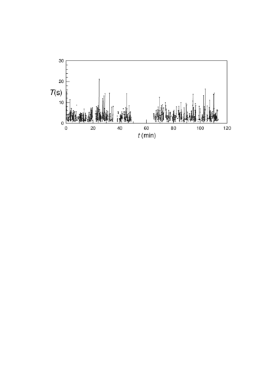
Figure 1: Time series of $T$ (time that elapses between consecutive touches). The match is Chelsea $\times$ Barcelona in 22/Feb./2006 (UEFA Champions League). Symbols are joined by linear segments whenever there is no interruption between touches.

Typical histograms of inter-touch times $T$ and increments $\Delta T$ (between consecutive inter-touch times) are presented in Fig. 2(a-b). Unless otherwise stated to the contrary, in this and subsequent analyses, touches of goal-keepers were not considered, because of the singular role in the game. These plots, built for the match of Fig. 1, are quite similar to those observed for other matches. In all cases the decay of the probability density function (PDF) of inter-touch times is approximately exponential and the PDF of increments presents a “tent” shape in the semi-log representation, suggesting a double exponential decay.

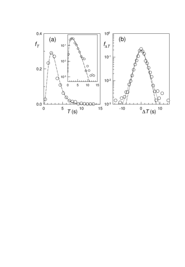
Figure 2: Normalized histograms of (a) inter-touch times and (b) their increments, for the match of Fig. 1. The inset in (a) is a semi-log representation of the same data plotted in the main frame. Dashed lines represent: (a) Gamma PDF given by Eq. (2) with parameters $\beta=3.43\pm 0.17$ and $\tau/$s$=0.85\pm 0.05$, and (b) the corresponding PDF of increments given by Eq. (4). The full line in (b) corresponds to Eq. (6).

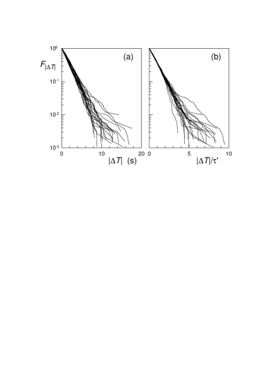
Figure 3: Cumulative distribution of increments. In (a) $F_{|\Delta T|}(t)=Prob(|\Delta T|\geq t)$ was computed for each of the twenty matches listed in Fig. 4. In (b), increments are scaled by the respective exponential decay time $\tau^{\prime}$ obtained from the exponential fit to each curve in (a), performed for values up to approx. $2\tau^{\prime}$ only.

Histograms of the increments, built for several matches, are exhibited in Fig. 3(a). Cumulative distributions were considered to reduce fluctuations. In order to quantitatively characterize each match, we calculated the exponential decay time $\tau^{\prime}$, since in all cases the initial decay is exponential. Calculation of $\tau^{\prime}$ was performed through an exponential fit to the cumulative distributions of increments over the interval $\Delta T<4s$. The fitting procedure, that will denominate WLS along the paper, was weighted least squares, with weights $w_{i}=1/|y_{i}|$ attributed to each data point $(x_{i},y_{i})$, and was performed by means of commercial software Origin. Fig. 3(a) already exhibits qualitatively the narrow statistical diversity found from one match to another, concerning the most frequent events. Constraints, such as rules of the game and human effort limitations, confine single realizations to a narrow spectrum. In fact, values of $\tau^{\prime}$ fall within the narrow interval $\tau^{\prime}=(1.89\pm 0.18$) s. Collapse of the re-scaled data is observed up to $|\Delta T|\simeq 2\tau^{\prime}$ only (Fig. 3(b)). Naturally, deviations from the mean behavior occur for large $\Delta T$ because events are rare.

III Modeling inter-touch time statistics

Let us consider the random variable $X_{t}$ representing the number of occurrences during the period $[0,t)$. If the stochastic process $\{X_{t},t>0\}$ were purely Poissonian (as commonly considered for arrival time statistics), with expected rate $1/\tau$, then the PDF of inter-touch times should be the exponential $f_{T}(t)={\rm e}^{-t/\tau}/\tau$ probs . Moreover, given two independent variables $T_{1}$, $T_{2}$ with the same exponential distribution, the increment $\Delta T=T_{2}-T_{1}$ has the so called double exponential or Laplace PDF

$$f_{\Delta T}(t)=\frac{1}{2\tau}{\rm e}^{-|t|/\tau}.$$ (1)

Although the distribution of increments $\Delta T$ is in good accord with a Laplace PDF, at least for central values, the distribution of inter-touch times $T$ is clearly not a pure exponential (see Fig. 2(a)). Therefore, the exponential, with one single fitting parameter, constitutes a very coarse model for the histograms of inter-touch times.

Instead, the time interval between touches can be thought to be composed, in average, of a certain number $\beta$ of independent phases. If each of the phases is $\tau$-exponentially distributed, then one obtains the Erlang distribution:

$$f_{T}(t)=\frac{1}{\tau\Gamma(\beta)}(t/\tau)^{\beta-1}{\rm e}^{-t/\tau}\equiv\Gamma_{\beta,\tau}(t),$$ (2)

defined for $t\geq 0$. This PDF is also known as gamma distribution, for real $\beta\geq 1$. In the particular case $\beta=1$, one recovers the pure exponential distribution. However, in the vicinity of the origin the PDF of inter-touch times has a shape compatible with $\beta>1$. In fact, very short inter-touch times are not frequent since players are not typically so close to each other. Very long inter-touch times are also scars since teams dispute ball possession almost all the time. Moreover, let us remark that the Erlang distribution is commonly used for modeling the distribution of times to perform some compound task, such as repairing a machine or completing a customer service task . Also in the present case, when a player receives the ball, it is common that he executes more than one task, such as, keeping possession of the ball, avoiding opponents, and passing the ball to another member of his team. In what follows we do not restrict $\beta$ to take integer values. Then $\beta$ can be interpreted as an average number of phases.

Fig. 2(a) shows the results of WLS fitting the gamma PDF to the numerical histograms of inter-touch times. We observe a clear improvement in the description of the statistics of inter-touch times, in comparison with the pure exponential model, for small and moderate times. Assuming a gamma distribution, parameters $\beta$ and $\tau$ were determined by means of a least square fit to empirical PDFs, using statistical weights in order to ponder the tails of the distributions. Even so, although a good description of numerical histograms is obtained for small and moderate values, there are important deviations at the tails. This also suggests that the gamma distribution may not be a very good model for the present data.

Fig. 4 exhibits the values of parameters $\beta$ and $\tau$ for several matches, together with the value of $\tau^{\prime}$ (for the cumulative distribution of increments). Values of $\tau$ are found within the interval $[0.68,1.06]$, with average value $0.91$, while $\beta$ values fall within the interval $[2.6,4.2]$, with mean $3.24$. There is a tendency that faster games (smaller $\tau$) are characterized by a larger $\beta$, as clearly observed in Fig. 4. There is also a trend that more decisive matches or matches played by highly ranked teams have smaller $\tau$ and larger $\beta$, e.g., PA, SL are final matches, AR, CB are usual matches of the UEFA champions league. These tendencies are expected because in such matches players usually save no efforts and strategies are more elaborated. If we assume that successive inter-touch times are independent identically gamma-distributed variables, then, the PDF of increments becomes

$$f_{\Delta T}(t)=\frac{{\rm e}^{-|t|/\tau}}{\tau^{2\beta}[\Gamma(\beta)]^{2}}\int_{0}^{\infty}[x(|t|+x)]^{\beta-1}{\rm e}^{-2x/\tau}\,dx\;.$$ (3)

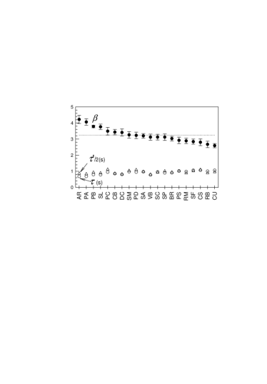
Figure 4: Parameters $\beta$ and $\tau$, obtained from the WLS fit of the gamma distribution to the histograms of inter-touch times, for the matches indicated in the abscissa axis (see Table 1 for letter code). Parameter $\tau^{\prime}$, obtained from cumulative histograms of increments is also exhibited. Matches were ranked by decreasing $\beta$.

Notice that this function has the same asymptotic behavior as the Laplace PDF but it is smoother at the origin. In particular, for $\beta=3$ (integer value closer to the average one), one gets

$$f_{\Delta T}(t)=\frac{1}{16\tau}\left[3+(3+|t|/\tau)|t|/\tau\right]{\rm e}^{-|t|/\tau}.$$ (4)

Once obtained the values of parameters $(\beta,\tau)$ for the distribution of inter-touch times, they were used to predict the PDF of increments by means of Eq. (3). From the results, shown in Fig. 2(b), one concludes that the prediction of the PDF of increments, assuming independence of consecutive inter-touch times, is satisfactory except at the tails.

Let us discuss some points that may be responsible for deviations from the simple Poissonian framework. First, we investigated the assumption of independence of occurrences in non-overlapping intervals. We calculated auto-correlation functions both for variables $T$ and $\Delta T$, taking into account the intrinsically discontinuous nature of the time series. Hence, only pairs of times belonging to the same sequence of touches were considered. No significant correlations were detected in the series of $T$, although the series of $\Delta T$ typically presents traits of antipersistence. Hence, despite the existence of strategies and patterns involving several players (some in cooperation and others in opposition), the lack of significant correlations indicates that memory effects in the succession of touches are very weak.

Another possibility for the failure of the simple Poissonian picture concerns stationarity and homogeneity. In order to investigate this aspect, we analyzed for each match the number of events $N$ as a function of time, as illustrated in Fig. 5. Beyond the discontinuity of the time series, temporal inhomogeneities throughout a match are common. First of all, average rates computed over each half of the matches are almost always different. In most of the cases, these average rates are larger in the first half, as soon as players are usually more tired in the second half of a match. At a finer time scale, small segments with different rate (slope) can be identified (especially during the first half, in the case of Fig. 5(a)). This feature is a manifestation of the change of rhythms throughout a match. We estimated local rates $\lambda\equiv 1/\tau$ as $\lambda=n/t_{IN}$, where $t_{IN}$ is the duration of each full sequence of ininterrupted touches and $n$ is the number of touches in that sequence. The histogram of rates $\lambda$ is shown in Fig. 5(b). Meanwhile panel (c) displays $\lambda$ as a function of time, putting into evidence its fluctuating character.

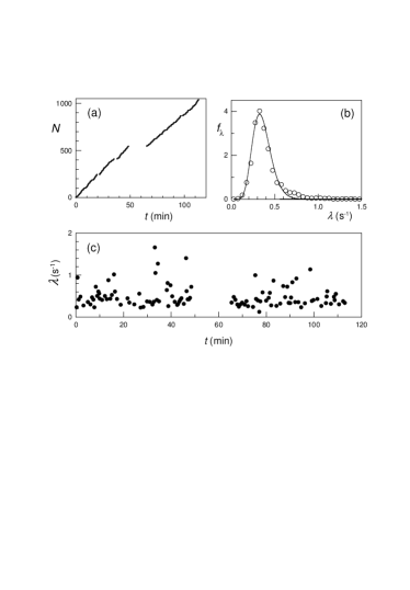
Figure 5: Number of events as a function of time (a), for the mathc of Fig. 1. Histogram of local rates $\lambda$ (b). Solid lines represent WLS fits of a gamma distribution $\Gamma_{\alpha,\kappa}$ with $(\alpha,\kappa/$s${}^{-1})=$ (11.1,0.032) Local rate $\lambda$ as a function of time (c).

We will see that the fact that the rate of occurrence $\lambda$ is not constant, but instead it is a fluctuating quantity, may explain the behavior of the tails of inter-touch time distributions. In effect, let us interpret the PDF $\Gamma_{\beta,1/\lambda}(t)$ as the conditional PDF $f_{T|\lambda}$ of variable $T$ given $\lambda$, where $\lambda$ is a stochastic variable. Moreover, let us also assume that $\lambda$ is gamma distributed, i.e., $f_{\lambda}(x)=\Gamma_{\alpha,\kappa}(x)$. Although this may be only a crude estimation of the distribution of local rates, it takes into account its main features, except deviations at the tails (see Fig. 5(b)). Under the assumptions above, the marginal PDF has the form beck1 ; beck0 ; beck2

$$f_{T}(t)=\int dxf_{\lambda}(x)f_{T|\lambda}(t,x)={\cal N}t^{\beta-1}{\rm e}_{q}^{-t/{\tau}},$$ (5)

where ${\cal N}$ is a normalization factor, $\tau=1/[(\alpha+\beta)\kappa]$, $q=1+1/(\alpha+\beta)$ and the $q$-exponential function (${\rm e}_{q}$) for negative argument is defined as ${\rm e}_{q}^{-x}=[1+(q-1)x]^{\frac{1}{1-q}}$, if $q>1$. This PDF that generalizes the gamma distribution, is known as $F$-distribution or also as $q$-gamma distribution silvio . Panel (a) of Fig. 6 shows the WLS fit of the $q$-gamma function to the same data of Fig. 2. In order to asses the goodness of fit we applied the Kolmogorov-Smirnoff test KS . We calculated confidence levels $\alpha$ by determining the largest deviation between the cumulative distribution that arises from WLS fit and the observed one. We obtained higher confidence levels for the $q$-gamma model. As illustration, for match CB, the gamma and $q$-gamma fits yielded $\alpha=7\%$ and 32%, respectively. Furthermore, the chi-square value of fit and the correlation coefficient for match CB were $(\chi^{2},R^{2}$)= (0.0009, 0.99) (against (0.002, 0.97) for the simple gamma distribution).

Although at the cost of introducing one more parameter, the $q$-gamma model is satisfactory for the full range of values. The advantage of introducing one more parameter was quantified through Akaike information criterium (AIC=$2k-2\ln L$, where $k$ is the number of parameters and $L$ the maximum likelihood) and also through Schwarz criterium (SIC=$k\ln(n)-2\ln L$, where $n$ is the number of observations), which penalizes more strongly the introduction of free parameters akaike . In all cases the $q$-gamma distribution yielded lower values. For example, (AIC, SIC)= (3726, 3741) (against (3760, 3772) obtained with the simple gamma) for CB and (82694, 82718) (against (83650, 83666)) for the global set.

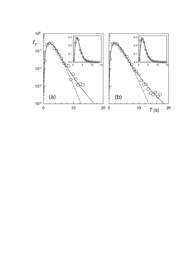
Figure 6: Normalized histograms of inter-touch times, (a) for the match of Fig. 1 and (b) for all the matches investigated. Dashed lines correspond to the gamma distribution with parameters ($\beta,\tau/$s)= ($3.43\pm 0.17$, $0.85\pm 0.05$) (a) and ($3.12\pm 0.12$, $0.95\pm 0.05$) (b). Solid lines correspond to the $q$-gamma distribution with parameters $(\beta,\tau/$s$,q$)= ($4.45\pm 0.35$,$0.43\pm 0.07,1.066\pm 0.007$) (a), ($4.20\pm 0.17$, $0.43\pm 0.04$,$1.076\pm 0.003$) (b). Insets: linear representations of the same data.

Furthermore the PDF of increments, which generalizes Eq. (3), namely,

$$f_{\Delta T}(t)\propto\int_{0}^{\infty}[x(|t|+x)]^{\beta-1}{\rm e}_{q}^{-x/\tau}{\rm e}_{q}^{-(|t|+x)/\tau}\,dx\;\,,$$ (6)

also describes better numerical data (see Fig. 2(b), where the full line is the predicted PDF of increments using the parameters of Fig. 6(a)).

In Fig. 6(b), all the matches were merged. In this case, the merging procedure by itself might give rise to the dispersion of $\lambda$ responsible for the behavior of the tails. This global analysis, however, is useful for characterizing the average behavior of football activity as a whole. Since, as observed before, diversity is not very high amongst matches, one observes for the merged data a behavior similar to that observed for a single match (illustrated in Fig. 6(a)), although the statistics is poorer in the later case.

The introduction of parameter $q$ allows to describe better the statistics of rare events. Notice that, in comparison with the gamma fits, the $q$-gamma ones yield $\beta$ about one unit larger and $\tau$ about one half smaller. Alternatively, assuming that the fluctuating rates obey a gamma distribution $\Gamma_{\alpha,\kappa}$, one can obtain $q$ (i.e., $q=1+1/(\alpha+\beta)$) and $\tau$ (i.e., $\tau=1/[(\alpha+\beta)\kappa]$) for the resulting $q$-gamma distribution. The values of $q$ are very close to those obtained by directly fitting the $q$-gamma distributions ($q\simeq 1.07$). Whereas, the resulting values of $\tau$ are larger than those obtained from $q$-gamma fits but still of the order of 1s. Therefore our model is selfconsistent. The lack of a complete matching of parameter $\tau$ is due to diverse reasons. On one hand, there is a certain degree of arbitrariness in the definition of local rates, that in our case were computed over each continuous sequence of touches, through $n/t_{IN}$. Moreover, the distribution of local rates as here defined are not strictly gamma, but only approximately. Finally, also parameter $\beta$ is an averaged quantity since the number of phases may fluctuate throughout a match. Nevertheless, the comparison between theoretical and empirical distributions supports the present model as a better approximation than the simple gamma distribution.

IV In and out-of-play intervals

In Fig. 7(a) we present the histogram of $t_{IN}$ (duration of the intervals without interruption). Notice that $t_{IN}=\sum_{i=1}^{n}T_{i}$. Then, its PDF can be obtained as $\rho(t_{IN})=\sum_{n\geq 1}\rho(t_{IN}|n)P(n)$, where $P(n)$ is the distribution of the number of touches $n$ in each continuous sequence. The conditional PDF is in first approximation $\Gamma_{\beta,n\tau}$, assuming that the $n$ inter-touch times are independent identically $\Gamma_{\beta,\tau}$ stochastic variables. On the other hand, $P(n)$ follows approximately the exponential law ${\rm e}^{-n/n_{o}}/n_{o}$ (Fig. 7(b)), being $n_{o}\simeq 7.54\pm 0.21$ (from WLS fit), while $\langle n\rangle\simeq 8.4\pm 0.3$. Under the assumptions above, one obtains a PDF that can be well approximated by an exponential with characteristic time $\tau_{IN}\simeq\langle n\rangle\beta\tau$, consistent with the numerical results in Fig. 7(a).

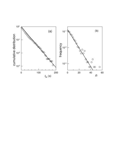
Figure 7: Statistics of in-play intervals. Cumulative histogram of $t_{IN}$ (a). The straight line corresponds to a exponential with characteristic time $\tau_{IN}=28s$. Normalized histogram of the number of touches in each continuous sequence (b).

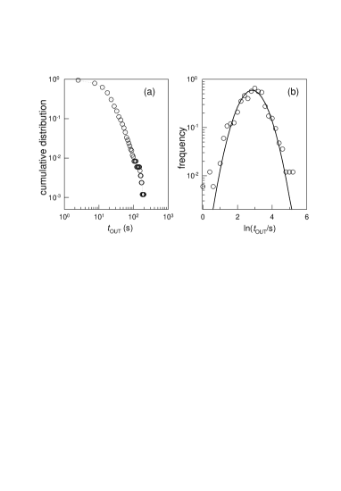
Figure 8: Statistics of out-of-play intervals. Cumulative histogram of $t_{OUT}$ (a). In (b), normalized histogram of $\ln t_{OUT}$ (symbols) and Gaussian fit with mean 2.85 and variance 0.45 (solid line).

The histogram of times elapsed between sequences (duration of intervals when the ball is out-of-play) was also computed and it is exhibited in Fig. 8(a). Since both $t_{IN}$ and $t_{OUT}$ statistics are poor over a single match (about one hundred events), we merged the records of several matches (AV,RA,MB,VZ,LF,BM,CB, following Table 1). In these cases goal-keeper movements were computed.

Although the statistics of out-of-play intervals appears to display a power-law behavior, a more careful analysis points to a log-normal statistics (Fig. 8(b)). Up to now, the results were well understood within the framework of non-homogeneous Poisson processes. However, in the case of out-of-play intervals, the PDF basically obeys a log-normal statistics that is not straightforwardly related to the previous scenario.

V Final observations

The statistics of touches can be understood on the basis of Poissonian arrival or point processes. Basically, events are not simply Poissonian but can be thought as composed of different phases, as also observed for compound tasks. This explains the behavior of the histogram of inter-touch times in the vicinity of the origin. Meanwhile, non-homogeneities in the rate of occurrence (changes of rhythm) throughout a match appear to be responsible for the power law tail in the distribution of inter-touch times, giving rise to a $q$-gamma function. It is noteworthy that a similar mechanism based on compound distributions for the obtention of such PDFs has been proposed within the context of the “superstatistics”beck1 , where the fluctuating parameter is the temperature. Here, we provide an example where $q$-gamma distributions arise as a consequence of the fluctuating nature of a relevant parameter.

All the main features here exhibited and discussed for the matches in Table 1 are also observed, in a preliminary analysis, for the sixty four matches of the 2006 World Cup (results not shown). Within the simple Poissonian framework, the effective characteristic time $\tau$ (of the order of one second) does not change significantly from one match to another. Meanwhile, parameter $\beta$ exhibits a greater variation, remaining approximately between 2 and 4, with average number of tasks close to 3. In general there is a tendency that $\tau$ is shorter and $\beta$ larger in more decisive matches or matches played by highly ranked teams. These trends are qualitatively expected as far as in such matches players usually save no efforts, playing faster and using more elaborated strategies. In fact, larger $\beta$ already suggests more developed or complex actions. The introduction of a further parameter, $q$, which reflects the degree of inhomogeneity of rhythms, improves the description of the tails. The statistics of the duration of sequences of touches, interrupted by fouls, ball leaving the field, etc., can also be derived within the same approach used for the statistics of touches.

On the other hand, the statistics of intervals between sequences of touches is of a different nature, belonging to the log-normal class. There are diverse mechanisms that may give rise to such statistics. As an example, for time series observed in turbulent flows, it has been attributed to a multiplicative random process beck2 . However this issue should be further investigated and deserves separate work.

	Match(cup)	Date		Match(cup)	Date
BR	Barcelona 1$\times$1 R.Madrid(S)	02/Apr./06	PA	São Paulo 4$\times$0 Atlético-PR(L)	14/Jul./05
RB	R.Sociedad 0$\times$2 Barcelona(S)	19/Mar./06	DC	D. Cali 0$\times$1 Corinthians(L)	15/Feb./06
AV	A.Bilbao 1$\times$1 Villareal(S)	26/Feb./06	CU	Corinthians 2$\times$2 U. Católica(L)	22/Feb./06
RA	R.Madrid 3$\times$0 Alaves(S)	19/Feb./06	PD	Palmeiras 2$\times$0 D. Táchira(L)	25/Jan./06
VB	Valencia 1$\times$0 Barcelona(S)	12/Feb./06	PB	Paraná 2$\times$0 Botafogo(B)	03/Aug./05
MB	Mallorca 0$\times$3 Barcelona(S)	29/Jan./06	PC	Paraná 1$\times$2 Corinthians(B)	14/Mar./06
VZ	Valencia 2$\times$2 Zaragoza(S)	19/Jan./06	CS	Corinthians 1$\times$3 São Paulo(B)	07/May/06
RM	Reggina 1$\times$4 Milan (I)	12/Feb./06	SA	Santos 2$\times$0 Atlético-PR(B)	23/Apr./06
LF	Leverkusen 2$\times$1 E. Frankfurt(G)	28/Jan./06	SF	São Paulo 1$\times$0 Flamengo(B)	16/Apr./06
BM	Borussia M. 1$\times$3 B. Munchen(G)	27/Jan./06	PS	P. Santista 0$\times$5 São Paulo(P)	12/Feb./06
CB	Chelsea 2$\times$1 Barcelona (E)	22/Feb./06	SP	Santos 1$\times$0 Palmeiras (P)	05/Mar./06
AR	Arsenal 0$\times$0 R. Madrid (E)	08/Mar./06	SC	S. Caetano 2$\times$1 Corinthians(P)	08/Feb./06
SL	São Paulo 1$\times$0 Liverpool(C)	18/Dec./05	SM	Santos 3$\times$2 Marília(P)	22/Jan./06

Table 1: Matches of South-American and European championships. Cups are B (Brazilian), C (FIFA World Club), E (UEFA Champions League), G (German), I (Italian), L (Libertadores), P (Brazilian, São Paulo State), S (Spanish).

Acknowledgements: We thank Brazilian agency CNPq for partial financial support. We also thank S. Picoli Jr. for interesting remarks.

References

- (1) L.C. Malacarne and R.S. Mendes, Physica A 286, 391(2000); J. Greenhough, P.C. Birch, S. C. Chapman and G. Rowlands, Physica A 316, 615 (2002).
- (2) J. Park and M.E.J. Newman, e-print physics/0505169.
- (3) M.E. Glickman and S. Hal, J. Am. Stat. Ass. 93, 25 (1998).
- (4) R.N. Onody and P.A. de Castro, Phys. Rev. E 70, 037103( 2004).
- (5) A. Borrie, G.K. Jonsson and M.S. Magnusson, Journal of Sports Sciences 20, 845 (2002); G. K. Jonsson, S.H. Bjarkadottir and B. Gislason, in Measuring Behavior 2000, 3rd International Conference on Methods and Techniques in Behavioral Research (pp. 168-171), L.P.J.J. Noldus Ed., Nijmegen, Netherlands (2000).
- (6) C. Beck and E.G.D. Cohen, Physica A 322, 267 (2003).
- (7) C. Tsallis, J. Stat. Phys. 52, 479 (1988); Nonextensive Mechanics and Thermodynamics, edited by S. Abe and Y. Okamoto, Lecture Notes in Physics Vol. 560 (Springer, Berlin, 2001); in Non-Extensive Entropy-Interdisciplinary Applications, edited by M. Gell-Mann and C. Tsallis, (Oxford University Press, Oxford, 2004).
- (8) W. Feller, An introduction to probability theory and its applications (Wiley, New York, 1968).
- (9) A.M. Law and W.D. Kelton, Simulation, modeling and analysis (McGraw-Hill, New York, 1991).
- (10) N.L. Jonhson and S. Kotz, Distribution in statistics: continuous univariate distributions (John Wiley & Sons, New York, 1970).
- (11) C. Beck, E.G.D. Cohen and H.L. Swinney, Phys. Rev. E 72, 056133 (2005).
- (12) S.M.D. Queirós, Europhysics Letters 71, 339 (2005); e-print physics/0411111; S.M.D. Queirós, C. Anteneodo and C. Tsallis, Noise and Fluctuations in Econophysics and Finance, eds. D. Abbott, J.-P. Bouchaud, X. Gabaix and J.L. McCauley, Proceedings of SPIE, 5848 (SPIE, Bellingham, WA, 2005) 151; C. Anteneodo and R. Riera, Phys. Rev. E 71, 201061 (2005).
- (13) J.H. Jerrold, Biostatistical analysis (Prentice Hall, New Jersey 1999); W.H. Press, B.P. Flannery, S.A. Teukolsky, W.T. Vetterling, Numerical Recipes. The Art of Scientific Computing (Cambridge University Press, Cambridge, 1986).
- (14) H. Akaike, IEEE Transactions on Automatic Control 19, 716 (1974); G. Schwarz, Annals of Statistics 6, 461 (1978).