Abstract

We present a detailed study of soliton compression of ultra-short pulses based on phase-mismatched second-harmonic generation (i.e., the cascaded quadratic nonlinearity) in bulk quadratic nonlinear media. The single-cycle propagation equations in the temporal domain including higher-order nonlinear terms are presented. The balance between the quadratic (SHG) and the cubic (Kerr) nonlinearity plays a crucial role: we define an effective soliton number – related to the difference between the SHG and the Kerr soliton numbers – and show that it has to be larger than unity for successful pulse compression to take place. This requires that the phase mismatch be below a critical level, which is high in a material where the quadratic nonlinearity dominates over the cubic Kerr nonlinearity. Through extensive numerical simulations we find dimensionless scaling laws, expressed through the effective soliton number, which control the behaviour of the compressed pulses. These laws hold in the stationary regime, in which group-velocity mismatch effects are small, and they are similar to the ones observed for fiber soliton compressors. The numerical simulations indicate that clean compressed pulses below two optical cycles can be achieved in a $\beta$-barium borate crystal at appropriate wavelengths, even for picosecond input pulses.

OCIS codes:  320.5520, 320.7110, 190.5530, 190.2620, 190.4400

1 Introduction

Second-harmonic generation (SHG) in the limit of large phase mismatch gives rise to the so-called cascaded $\chi^{(2)}:\chi^{(2)}$-nonlinearity, in which weak conversion to the second harmonic (SH) occurs, while a Kerr-like nonlinear phase shift is induced on the fundamental wave (FW) [1, 2]. An elegant theoretical view of this process is that in the cascading limit the system can be described by a nonlinear Schrödinger equation (NLSE) for the FW alone [3]. The induced FW nonlinear phase shift then comes from an effective self-phase modulation arising from the phase mismatch. The phase shift can be quite large and negative, since the phase mismatch determines the sign and magnitude of the effective cubic nonlinearity. Such a self-defocusing nonlinearity can be used to compress a pulse when combined with normal dispersion [4, 5, 6, 7, 8, 9], and problems normally encountered due to self-focusing in cubic media are avoided. Thus, having no power limit, a self-defocusing compressor can create high-energy near single-cycle fs pulses in bulk media [4, 8]. The exploited compression mechanism is the periodic behaviour of higher-order temporal solitons of the NLSE. They oscillate in temporal duration upon propagation, and the optimal compressor length is when the pulse width is the narrowest.

As the compressor scheme exploits an effective self-defocusing cubic term from cascaded quadratic effects, the compressor will naturally be affected by the self-focusing cubic nonlinearity inherent to any transparent material. This detrimental cubic nonlinearity must be counterbalanced and then exceeded to achieve compression [5, 8]. In this work we systematically demonstrate theoretically and numerically how this can be expressed conveniently using the soliton number formalism known from the NLSE in fiber optics [10, 11]. Firstly, we show that the SHG soliton number [8] $N_{\rm SHG}$ must outbalance the Kerr soliton number $N_{\rm Kerr}$ before compression takes place. More precisely, the effective soliton number $N_{\rm eff}=\sqrt{N_{\rm SHG}^{2}-N_{\rm Kerr}^{2}}$ must be larger than unity. This can be achieved by adjusting the phase mismatch, but only if the quadratic material nonlinearity is sufficiently stronger than the cubic Kerr nonlinearity. Secondly, when compression is successful, the compression factor, pulse quality, and optimal compressor length follow certain scaling laws. Such empirical scaling laws expressed through $N_{\rm Kerr}$ were previously given for the NLSE [12, 13, 14]. Here we present detailed numerical simulations of pulse propagation in a commonly-used nonlinear material, $\beta$-barium borate (BBO). We find general dimensionless scaling laws quite similar to the ones from the NLSE, except that one must express them through $N_{\rm eff}$. The simulations span a very wide input-pulse parameter space and the scaling laws therefore provide an important tool for experimental situations.

A major obstacle to the cascaded-quadratic soliton compressor is the group-velocity mismatch (GVM) between the FW and SH pulses. GVM induces a Raman-like perturbation that distorts the compression, resulting in asymmetric pulses and pulse splitting [4, 15, 8]. Two distinct regimes exist: in the stationary regime the GVM-induced Raman-like perturbations are weak, resulting in clean compressed pulses. In the nonstationary regime, the GVM-induced perturbations are strong, and poor pulse compression is observed. Moreover, the compression behavior deviates from the NLSE scaling laws. Here we focus on the stationary regime, where cleanly compressed few-cycle pulses may be obtained, and summarize the guidelines for avoiding nonstationary behavior. Subsequent publications will focus on compression in the nonstationary regime in greater detail. In particular, we have recently devised a nonlocal theory that quantitatively defines the boundary between the stationary and nonstationary regimes [16].

Finally, when describing (ultra)-short pulse propagation in nonlinear media it is generally important to describe both temporal and spatial effects as they will inherently be interlinked. Examples include space-time focusing in bulk media [17], and strong modification of the dispersion and nonlinear mode overlap in waveguide geometries. However, the simplified 1D temporal description presented here is often an adequate starting point for understanding the general temporal behaviour of the system during compression. In this work we consider interaction in a bulk material (no wave guiding) and we neglect diffraction (i.e., the beam must not be focused too tightly). In subsequent publications we will address the behaviour in a wave-guiding geometry such as a fiber, as well as in bulk geometry including the spatial effects.

2 Generalized propagation equations for ultra-short pulses

Below we present the generalized bulk SHG propagation equations, including both quadratic and cubic nonlinear effects. We aim to investigate compressed pulses that may be near-single optical cycle in duration, so we must use the propagation equations derived without approximations that directly impart constraints on the pulse duration and bandwidth. Such SHG equations have been derived elsewhere [18] using the slowly evolving wave approximation (SEWA) [17]. Here we recast these equations in the framework of cascaded quadratic soliton compression as to define all critical experimental parameters. We also include generalized cubic nonlinearities from interaction of two fields with different frequencies (the FW and SH), see App. A.

The investigation is a temporal study only. We neglect transverse spatial effects, assuming that diffraction plays a negligible role on the length scale of the compressor, i.e., that each point on the beam may be considered a plane wave. Previously-reported quadratic soliton compressors have lengths on the order of a few centimeters [4, 5, 6, 7, 8]. For a Gaussian beam at near-infrared wavelengths, this implies that our assumptions are valid for beam waists larger than approximately 100 $\mu$m. Section F will discuss considerations of compression with transverse-spatially varying profiles. Finally note that in our notation, a primed variable is always dimensionless.

A The dimensional form

In SHG two FW photons of frequency $\omega_{1}$ combine to give a photon of frequency $\omega_{2}=2\omega_{1}$ (the SH). We consider scalar fields and either a Type-0 or Type-I SHG geometry, in which the two FW photons have identical polarization [19]. In a bulk medium, the generalized SEWA propagation equations for the coupled electric fields are

$$\hat{\mathcal{L}}_{1}E_{1}+\kappa_{\rm SHG,1}^{E}\hat{S}_{1}E_{1}^{*}E_{2}e^{i\Delta kz}+\kappa_{\rm Kerr,1}^{E}\times$$ (1a)

$$\left[(1-f_{R})\hat{S}_{1}E_{1}\left(|E_{1}|^{2}+B|E_{2}|^{2}\right)+f_{R}\mathcal{R}_{1}(\tau)\right]=0,$$

$$\hat{\mathcal{L}}_{2}E_{2}+\kappa_{\rm SHG,2}^{E}\hat{S}_{2}E_{1}^{2}e^{-i\Delta kz}+\kappa_{\rm Kerr,2}^{E}\times$$ (1b)

$$\left[(1-f_{R})\hat{S}_{2}E_{2}\left(|E_{2}|^{2}+B|E_{1}|^{2}\right)+f_{R}\mathcal{R}_{2}(\tau)\right]=0,$$

where $E_{j}=E_{j}(z,t)$. For a Type-0 geometry the cross-phase modulation (XPM) coefficient is $B=2$, while for a Type-I geometry $B=2/3$ because the FW and SH have orthogonal polarization [11]. We assume that the FW and SH spectra do not significantly overlap, an assumption generally valid down to single-cycle pulse durations. The linear propagation operators are

$$\hat{\mathcal{L}}_{1} \equiv i\frac{\partial}{\partial z}+\hat{\mathcal{D}}_{1},$$ (2a)

$$\hat{\mathcal{L}}_{2} \equiv i\frac{\partial}{\partial z}-id_{12}\frac{\partial}{\partial\tau}+\hat{\mathcal{D}}_{2,\rm eff},$$ (2b)

where $\hat{D}_{j}$ are the dispersion operators

$$\hat{\mathcal{D}}_{j}\equiv\sum_{m=2}^{\infty}i^{m}\frac{k_{j}^{(m)}}{m!}\frac{\partial^{m}}{\partial\tau^{m}},$$ (3)

Here $k_{j}=n_{j}\omega_{j}/c$, where $n_{j}$ is the refractive index. The fields are in the frame of reference traveling with the FW group velocity $v_{g,1}$ by the transformation $\tau=t-z/v_{g,1}$. This is the origin of the GVM-term $d_{12}=1/v_{g,1}-1/v_{g,2}$, where $v_{g,j}^{-1}=k^{(1)}_{j}$. $k_{j}^{(m)}\equiv\partial^{m}k_{j}/\partial\omega^{m}|_{\omega=\omega_{j}}$ accounts for dispersion, and $\Delta k\equiv k_{2}-2k_{1}$ is the phase mismatch. Note the unfamiliar term in Eq. (2b), which is an effective SH dispersion operator $\hat{\mathcal{D}}_{2,\rm eff}=\hat{\mathcal{D}}_{2}+\hat{S}_{2}^{-1}\frac{d_{12}^{2}}{2k_{2}}\frac{\partial^{2}}{\partial\tau^{2}}$ [see Eq. (26)], which deviates from $\hat{\mathcal{D}}_{2}$ due to GVM and self-steepening in the SEWA model [18], see App. B.

The quadratic nonlinear coefficient is $\kappa_{{\rm SHG},j}^{E}\equiv\chi^{(2)}\omega_{1}/2cn_{j}=d_{\rm eff}\omega_{1}/cn_{j}$ where $\chi^{(2)}$ is the value of the quadratic nonlinear tensor along the polarization direction of the interacting waves, and as is typical we take $d_{\rm eff}\equiv\chi^{(2)}/2$. Dispersion of $\chi^{(2)}$ is assumed negligible.

The cubic nonlinear coefficient is $\kappa_{{\rm Kerr},j}^{E}=\omega_{j}n_{{\rm Kerr},j}/c$. The Kerr nonlinear refractive index is $n_{{\rm Kerr},j}\equiv 3{\rm Re}(\chi^{(3)})/8n_{j}$, where $\chi^{(3)}=\chi^{(3)}_{xxxx}$, see App. A. We neglect two-photon absorption, implying ${\rm Im}(\chi^{(3)})=0$, which holds as long as the SH frequency spectrum lies below the two-photon absorption edge of the medium. Note, the usual notation for $n_{{\rm Kerr},j}$ is $n_{2}$, but we reserve the subscript 2 for the SH.

Self-steepening effects are modelled by the operator $\hat{S}_{j}\equiv 1+\frac{i}{\omega_{j}}\frac{\partial}{\partial\tau}$, It approaches unity when bandwidths $\Delta\omega_{j}$ are small compared to the carrier frequencies $\omega_{j}$, i.e., for pulses longer than roughly 10 optical cycles.

Finally, $\mathcal{R}_{j}(\tau)$ describes the vibrational Raman response of the cubic nonlinearity, see App. A. We henceforth set $f_{R}=0$, because Raman scattering plays a negligible role under the relevant experimental conditions.

We now scale the fields by defining $A_{j}\equiv E_{j}\sqrt{\varepsilon_{0}n_{j}c/2}$ so $|A_{j}|^{2}$ gives the beam intensity $I_{j}$. Eqs. (1) become

$$\hat{\mathcal{L}}_{1}A_{1} +\kappa_{\rm SHG}^{I}\hat{S}_{1}A_{1}^{*}A_{2}e^{i\Delta kz}$$ (4a)

$$+\gamma_{1}^{I}\hat{S}_{1}A_{1}\left(|A_{1}|^{2}+B\bar{n}|A_{2}|^{2}\right)=0,$$

$$\hat{\mathcal{L}}_{2}A_{2} +\kappa_{\rm SHG}^{I}\hat{S}_{2}A_{1}^{2}e^{-i\Delta kz}$$ (4b)

$$+2\bar{n}^{2}\gamma_{1}^{I}\hat{S}_{2}A_{2}\left(|A_{2}|^{2}+B\bar{n}^{-1}|A_{1}|^{2}\right)=0.$$

The nonlinear coefficients due to the intensity scaling are $\kappa_{\rm SHG}^{I}\equiv\sqrt{2\omega_{1}^{2}d_{\rm eff}^{2}/n_{1}^{2}n_{2}\varepsilon_{0}c^{3}}$, and $\gamma_{1}^{I}\equiv\omega_{1}n_{{\rm Kerr},1}^{I}/c$. Here the intensity-version of the Kerr nonlinear refractive index with unit $[{\rm m^{2}/W}]$ is $n_{{\rm Kerr},1}^{I}\equiv 2n_{{\rm Kerr},1}/n_{1}\varepsilon_{0}c=3{\rm Re}(\chi^{(3)})/4n_{1}^{2}\varepsilon_{0}c.$ Note the connection to the fiber NLSE (where $A_{j}$ is scaled to the power); $\gamma_{1}^{I}$ is equivalent to the parameter [10] $\gamma_{1}=\omega_{1}n_{\rm Kerr,1}^{I}/cA_{\rm eff}$, where $A_{\rm eff}$ is the effective mode area of the FW. Finally, $\bar{n}\equiv n_{1}/n_{2}$ which is typically close to unity, except when $\Delta k$ is large.

B The dimensionless form

We now rescale space and time as $z^{\prime}\equiv z/L_{\rm D,1}$, and $\tau^{\prime}=\tau/T_{1,\rm in}$, where $L_{\rm D,1}\equiv T_{1,\rm in}^{2}/|k^{(2)}_{1}|$ and $T_{1,\rm in}$ are the FW dispersion length and input pulse duration. When compressing a FW pulse, no SH is launched, so both fields are scaled to the peak FW input intensity $I_{1,\rm in}\equiv|A_{1}(0,0)|^{2}$, i.e., $U_{j}=A_{j}/\sqrt{I_{1,\rm in}}$. Thus, $U_{1}=E_{1}/{\mathcal{E}}_{1,\rm in}$, where ${\mathcal{E}}_{1,\rm in}\equiv|E_{1}(0,0)|$, and Eqs. (4) become

$$\hat{\mathcal{L}}_{1}^{\prime}U_{1} +N_{\rm SHG}\sqrt{|\Delta k^{\prime}|}\hat{S}_{1}^{\prime}U_{1}^{*}U_{2}e^{i\Delta k^{\prime}z^{\prime}}$$ (5a)

$$+N_{\rm Kerr}^{2}\hat{S}_{1}^{\prime}U_{1}\left(|U_{1}|^{2}+B\bar{n}|U_{2}|^{2}\right)=0,$$

$$\hat{\mathcal{L}}_{2}^{\prime}U_{2} +N_{\rm SHG}\sqrt{|\Delta k^{\prime}|}\hat{S}_{2}^{\prime}U_{1}^{2}e^{-i\Delta k^{\prime}z^{\prime}}$$ (5b)

$$+2\bar{n}^{2}N_{\rm Kerr}^{2}\hat{S}_{2}^{\prime}U_{2}\left(|U_{2}|^{2}+B\bar{n}^{-1}|U_{1}|^{2}\right)=0,$$

where $N_{\rm SHG}$ and $N_{\rm Kerr}$, the dimensionless quadratic and cubic soliton numbers, respectively, are defined as

$$N_{\rm SHG}^{2} =L_{\rm D,1}\frac{\omega_{1}^{2}d_{\rm eff}^{2}{\mathcal{E}}_{1,\rm in}^{2}}{c^{2}n_{1}n_{2}|\Delta k|},$$ (6a)

$$N_{\rm Kerr}^{2} =L_{\rm D,1}\gamma_{1}^{I}I_{1,\rm in}=L_{\rm D,1}\omega_{1}n_{{\rm Kerr},1}^{I}I_{1,\rm in}/c,$$ (6b)

and the dimensionless phase mismatch is $\Delta k^{\prime}\equiv\Delta kL_{\rm D,1}$. The parameter $N_{\rm SHG}$ is deliberately chosen for a soliton compression scenario, as will become clear later.

Equations (2) on dimensionless form are $\hat{\mathcal{L}}_{1}^{\prime}\equiv i\frac{\partial}{\partial z^{\prime}}+\hat{\mathcal{D}}^{\prime}_{1},$ and $\hat{\mathcal{L}}_{2}^{\prime}\equiv i\frac{\partial}{\partial z^{\prime}}-id_{12}^{\prime}\frac{\partial}{\partial\tau^{\prime}}+\hat{\mathcal{D}}^{\prime}_{2,\rm eff}$, and $\hat{\mathcal{D}}^{\prime}_{2,\rm eff}$ is given by Eq. (27). The dimensionless dispersion operators and corresponding coefficients are $\hat{\mathcal{D}}_{j}^{\prime}\equiv\sum_{m=2}^{m_{d}}i^{m}\delta_{j}^{(m)}\frac{\partial^{m}}{\partial\tau^{\prime m}}$, and $d_{12}^{\prime}\equiv d_{12}T_{1,\rm in}/|k^{(2)}_{1}|$, and $\delta_{j}^{(m)}\equiv L_{\rm D,1}k_{j}^{(m)}(T_{1,\rm in}^{m-2}|k^{(2)}_{1}|m!)^{-1}$ Finally, using $s^{\prime}\equiv(\omega_{1}T_{1,\rm in})^{-1}$ we have the steepening operators with dimensionless time $\hat{S}_{1}^{\prime}\equiv 1+is^{\prime}\frac{\partial}{\partial\tau^{\prime}}$, and $\hat{S}_{2}^{\prime}\equiv 1+i\frac{s^{\prime}}{2}\frac{\partial}{\partial\tau^{\prime}}.$

C The soliton numbers

We now turn our attention to the soliton numbers as defined in Sec. B. We will argue – and later show with numerical simulations – that the effective soliton number $N_{\rm eff}=\sqrt{N_{\rm SHG}^{2}-N_{\rm Kerr}^{2}}$ can be used to describe the system in general. Indeed, $N_{\rm eff}$ characterizes the outcome for any given input state of the system.

First, consider the NLSE in absence of quadratic nonlinearities. We include for instruction the Raman terms and ignore the steepening terms [Eq. (25a) with $\kappa_{{\rm SHG},1}^{E}=0$ and $\hat{S}_{j}=1$]. In dimensionless form it reads:

$$i\frac{\partial U_{1}}{\partial z^{\prime}}-\frac{{\rm sgn}(k^{(2)}_{1})}{2}\frac{\partial^{2}U_{1}}{\partial\tau^{\prime 2}}\\ +N_{\rm Kerr}^{2}\left[|U_{1}|^{2}U_{1}-\tau^{\prime}_{R}U_{1}\frac{\partial|U_{1}|^{2}}{\partial\tau^{\prime}}\right]=0,$$ (7)

which holds when the pulse duration is much slower than the Raman response, and $\tau^{\prime}_{R}=\tau_{R}/T_{1,\rm in}$, where $\tau_{R}$ is a characteristic Raman vibrational response time [10], see App. A. The Kerr soliton number (6b) we express as $N_{\rm Kerr}\equiv\sqrt{L_{\rm D,1}/L_{\rm Kerr}}$, where $L_{\rm Kerr}=(\gamma_{1}^{I}I_{1,\rm in})^{-1}$ is the characteristic Kerr length. Equation (7) governs soliton compression in cubic nonlinear media, and the compression characteristics are well understood to be critically dependent on $N_{\rm Kerr}$ [10, 11, 12, 13, 14]. We stress that soliton compression using a pure Kerr self-focusing nonlinearity requires anomalous dispersion ${\rm sgn}(k^{(2)}_{1})<0$.

Likewise, the quadratic soliton number $N_{\rm SHG}$ is a critical parameter in cascaded quadratic soliton compression that as we shall now see has a role analogous to the cubic soliton number of the NLSE. Using perturbative methods one can reduce the dimensionless SHG equations (5) – in absence of steepening and cubic nonlinear terms – to a single equation for the FW analogous to Eq. (7) when the phase mismatch $\Delta k$ is suitably large [3, 15]. The approximate equation for the FW field can for soliton compression purposes be cast as [8]

$$i\frac{\partial U_{1}}{\partial z^{\prime}}-\frac{{\rm sgn}(k^{(2)}_{1})}{2}\frac{\partial^{2}U_{1}}{\partial\tau^{\prime 2}}-{\rm sgn}(\Delta k)\times\\ N_{\rm SHG}^{2}\left[|U_{1}|^{2}U_{1}+is_{12}\tau^{\prime}_{R,{\rm SHG}}|U_{1}|^{2}\frac{\partial U_{1}}{\partial\tau^{\prime}}\right]=0,$$ (8)

where $s_{12}={\rm sgn}(d_{12})$. In analogy to the cubic nonlinearity, a characteristic length for the cascaded quadratic nonlinearity $L_{\rm SHG}\equiv c^{2}n_{1}n_{2}|\Delta k|/\omega_{1}^{2}d_{\rm eff}^{2}{\mathcal{E}}_{1,\rm in}^{2}$, such that $N_{\rm SHG}\equiv\sqrt{L_{\rm D,1}/L_{\rm SHG}}$. The similarity to Eq. (7) is clear, and explains the choice of $N_{\rm SHG}$ in Eq. (6a). Similar to $N_{\rm Kerr}$ for the NLSE, $N_{\rm SHG}$ is namely a critical parameter in cascaded quadratic soliton compression. Several other features should be noted. First, the sign of the phase mismatch controls the sign of the induced cubic nonlinearity. For the purpose of soliton compression with normal dispersion ${\rm sgn}(k^{(2)}_{1})>0$, we require $\Delta k>0$ in order to have self-defocusing, or negative nonlinearity. Second, the Raman-like term in Eq. (8) is important in the compression dynamics, as will be explained in Sec. D.

Equations (7) and (8) consider the cases where either the cubic or the quadratic nonlinearity is significant. However, we must consider both orders of nonlinearity, so using the same perturbation methods, we reduce Eqs. (5) to an approximate equation for the FW. To first order, and neglecting steepening effects, we find

$$i\frac{\partial U_{1}}{\partial z^{\prime}}-\frac{{\rm sgn}(k^{(2)}_{1})}{2}\frac{\partial^{2}U_{1}}{\partial\tau^{\prime 2}}\\ -{\rm sgn}(\Delta k)N_{\rm SHG}^{2}\left[|U_{1}|^{2}U_{1}+is_{12}\tau^{\prime}_{R,{\rm SHG}}|U_{1}|^{2}\frac{\partial U_{1}}{\partial\tau^{\prime}}\right]\\ +N_{\rm Kerr}^{2}\left[|U_{1}|^{2}U_{1}-\tau^{\prime}_{R}U_{1}\frac{\partial|U_{1}|^{2}}{\partial\tau^{\prime}}\right]=0.$$ (9)

In Eq. (9) self-phase modulation (SPM) effects from both quadratic and cubic nonlinear effects are present. For $\Delta k>0$, $\chi^{(2)}:\chi^{(2)}$ self-defocusing phase shifts starts to cancel the $\chi^{(3)}$ self-focusing phase shifts. Thus, for soliton compression with normal dispersion and self-defocusing phase shifts, the effective soliton number

$$N_{\rm eff}^{2} \equiv N_{\rm SHG}^{2}-N_{\rm Kerr}^{2}$$

$$=L_{\rm D,1}{\mathcal{E}}_{1,\rm in}^{2}\frac{\omega_{1}}{c}\left(\frac{\omega_{1}}{c\Delta k}\frac{d_{\rm eff}^{2}}{n_{1}n_{2}}-n_{{\rm Kerr},1}\right),$$ (10)

must be larger than unity, $N_{\rm eff}>1$. This is analogous to the cubic soliton compressor, for which compression will only occur for $N_{\rm Kerr}>1$. In Sec. 3 these conclusions are supported numerically through simulations of Eqs. (5). By this we demonstrate that $N_{\rm eff}$ governs all the behaviour of the compressed solitons, at least in the stationary regime. This regime is now discussed.

D The stationary regime

An important observation is that Eq. (9) has a GVM-induced Raman-like term similar to the one induced by the delayed cubic response in the NLSE (7). Its characteristic dimensionless temporal response is [15, 8]

$$\tau^{\prime}_{R,{\rm SHG}}\equiv 2|d_{12}|/|\Delta k|T_{1,\rm in},$$ (11)

and $\tau^{\prime}_{R,{\rm SHG}}=\tau_{R,{\rm SHG}}/T_{1,\rm in}$. Typically, $\tau_{R,{\rm SHG}}$ lies between 1-5 fs in BBO. This term imposes a Raman-like red-shift of the FW, which causes the compressed pulse to be asymmetric and limits the compression achievable.

To understand this better, observe the effective nonlinear FW phase shift built up during propagation $\phi_{\rm NL}(z)\equiv-{\rm sgn}(\Delta k)z/L_{\rm SHG}=-z\omega_{1}^{2}d_{\rm eff}^{2}{\mathcal{E}}_{1,\rm in}^{2}/c^{2}n_{1}n_{2}\Delta k$ [1], which holds when $\sqrt{|\Delta k|L_{\rm SHG}}\gg 1$ (weak conversion to the SH). For efficient compression $\phi_{\rm NL}$ should at least be on the order of $-\pi$ [4, 5], and evidently the pulse needs to propagate a shorter distance to achieve this for $\Delta k$ low (as long as the cascading limit is upheld). However, Liu et al. [4] pointed out that GVM sets a lower limit to $\Delta k$: In phase-mismatched SHG, the phase between the FW and SH changes several times, corresponding to a conversion/back-conversion cycle of energy between FW and SH fields. The distance over which the relative phase changes sign once is exactly characterized by the coherence length $L_{\rm coh}=\pi/|\Delta k|$. Thus, it is important that the temporal walk-off (GVM) length $L_{\rm GVM}\equiv T_{1,\rm in}/|d_{12}|$ is (much) larger that the coherence length. Liu et al. [4] found that it is sufficient to demand that $L_{\rm coh}<4L_{\rm GVM}$. Thereby the so-called stationary regime was defined, thus requiring $\Delta k>4\pi|d_{12}|/T_{1,\rm in}$. Therefore it is advantageous to have low GVM because it gives access to large nonlinear phase shifts that occur when $\Delta k$ is not too large. In addition, low GVM will result in a smaller $\tau^{\prime}_{R,{\rm SHG}}$-term in Eq. (9) so the Raman-like perturbations become smaller. This was a main point of Ref. [8], where it was shown that for a given amount of GVM the compression increases as the soliton number is increased until a certain critical value where the Raman-like perturbations start to dominate. If GVM is reduced the soliton number can be increased further before this happens, and stronger compression can be achieved. We recently devised a more accurate theory for the stationary and nonstationary regimes [16], showing that the cascaded nonlinearity gives rise to a nonlocal response, and that in presence of GVM the nonlocal response function is asymmetric (Raman-like). In the stationary regime the nonlocal response function is localized and Eq. (9) is recovered in the weakly nonlocal regime (where the response function is very narrow compared to the propagating pulse). In the nonstationary regime the nonlocal response function is oscillatory and does not decay. This has severe consequences to the built up negative nonlinear phase shift and results in very poor compression. Finally, a more accurate requirement for being in the stationary regime was found as

$$\Delta k>\Delta k_{\rm sr}\equiv d_{12}^{2}/2k^{(2)}_{2},$$ (12)

which notably is independent of $T_{1,\rm in}$. In what follows, we will use this value. We should note that satisfaction of inequality (12) does not eliminate the GVM-induced perturbation: Raman-like effects are present when GVM is nonzero both in the stationary regime $\Delta k>\Delta k_{\rm sr}$, where Eq. (9) holds, and in the nonstationary regime $\Delta k<\Delta k_{\rm sr}$. However, in the latter case, where the nonlocal response function is oscillatory and unbound, the Raman-like perturbations are stronger.

E The compression window

In the previous sections we have imposed two requirements for clean soliton compression. First, in order to observe solitons, the effective soliton number must be larger than unity $N_{\rm eff}>N_{\rm eff,c}=1$. This gives from Eq. (10) a critical value of the phase mismatch

$$\Delta k<\Delta k_{c}=\frac{\omega_{1}d_{\rm eff}^{2}}{cn_{1}n_{2}n_{{\rm Kerr},1}(1+N_{\rm Kerr}^{-2})}.$$ (13)

Second, $\Delta k>\Delta k_{\rm sr}$ to be in the stationary regime, see Eq. (12), which is strictly related to the size of GVM and SH group-velocity dispersion, and is independent of the input pulse duration. This defines a compression window, inside which we can expect clean compression:

$$\Delta k_{\rm sr}<\Delta k<\Delta k_{c}.$$ (14)

Staying inside this window is therefore a question of choosing the right phase mismatch. Keeping the window open ($\Delta k_{\rm sr}<\Delta k_{c}$) is also a matter of having the right input pulse intensity and duration, see Fig. 1. Moreover, there are cases where the material nonlinearity balance and/or GVM effects do not allow for Eq. (14) to be satisfied. For instance, although $\Delta k_{c}$ increases with the input intensity, see Fig. 1(a), its maximum value, occurring when $N_{\rm Kerr}^{-2}\rightarrow 0$, is $\Delta k_{c,\rm max}=\omega_{1}d_{\rm eff}^{2}/cn_{1}n_{2}n_{{\rm Kerr},1}$. Thus, the balance between quadratic and cubic nonlinearities is a fundamental limit on the peak value of $\Delta k_{c}$. Moreover, when GVM is large $\Delta k_{\rm sr}$ becomes high, so very large quadratic nonlinearities are needed to open the window. Note that compression can be achieved outside the compression window when $\Delta k<\Delta k_{\rm sr}$. However, due to the strong Raman-like effects in the nonstationary regime $N_{\rm eff}$ must be kept small in order to get a clean symmetric pulse, allowing only for moderate compression. Conversely, even inside the compression window distorted compressed pulses may occur [16].

Fig. 1: The compression window for BBO with $\lambda_{1}=1064$ nm using (a) $T_{1,\rm in}=200$ fs, and (b) $I_{1,\rm in}=200~{}{\rm GW/cm^{2}}$. Also shown is $\Delta k_{c}$ found in numerics (see Sec. A), and the dashed line is an empirical scaling law (15) based on these simulations.

F Transverse spatial effects

Let us end with a brief discussion of the implications of including effects of modulation in the transverse spatial dimensions ($x$ and $y$). The equations will then include both diffraction terms and space-time focusing terms (due to steepening effects of diffraction [17]). In its simplest effect, diffraction will act to alter the pulse intensity by altering the mode area, which will lead to changes in the soliton order during propagation. Therefore, when $z_{0}$ is on the order of a characteristic diffraction length or longer, diffraction will have significant effects on the compression results. Additionally, the space-time focusing terms, which couple temporal and transverse spatial coordinates and become significant at few-cycle pulse durations, will be expected to produce nontrivial spatiotemporal distortions.

Moreover, in the plane-wave limit, i.e., where diffraction effects are small, while the temporal dynamics can be well described by the model presented in this paper, inhomogeneity in the spatial intensity profile will result in inhomogeneous compression across the beam. For example, for a Gaussian profile only the central part of the beam may have the appropriate intensity to be efficiently compressed. In order to achieve a more homogeneous compression, a super-Gaussian profile can be used [20].

Another case is where the light is guided, such as in an optical fiber. Here, the nonlinear terms in the propagation equations must include the effective spatial mode overlap areas, and thus modifying the soliton numbers as well. Another important difference in the guided case is that the dispersion is affected. Moreover, it is possible to achieve very high intensities with low energy pulses because the light can be confined in a very small area. We will in another publication go into details with the specific case of a photonic crystal fiber, and try to investigate the implications of wave-guiding effects on the cascaded quadratic soliton compressor.

3 Numerical results

We now proceed to the numerical results, where we first study the transition to compression, and then derive the empirical scaling laws for the compressed pulses. The simulations were done using Eqs. (5), which include self-steepening, the SEWA corrected SH dispersion term and higher-order nonlinear mixing terms. The coupled equations were solved using a split-step Fourier technique with a 2nd order Runge-Kutta algorithm to evaluate the nonlinear terms in the time domain. The dispersion terms were evaluated in the frequency domain, and since $k_{j}(\omega)$ is known analytically (from the Sellmeier equations of BBO [19]) we can actually evaluate the dispersion operator $\hat{D}_{j}$ exactly [21] instead of using the expansions (3). For the effective SH operator (27) we used 30 terms in the expansion of $\hat{S}_{2}^{-1}$.The steepening terms were applied by using the convolution theorem and thus letting the steepening operator act on the nonlinear terms in the frequency domain. The number of discretization points $N_{z}$ in the $z$-direction was chosen so that around 15 steps were taken within a single coherence length $L_{\rm coh}=\pi/|\Delta k|$. The number of temporal points were $2^{12}$-$2^{15}$, primarily dictated by the fact that due to GVM the SH will have a trailing pulse, which must stay inside the time window of the simulations.

We decided to use BBO as the nonlinear medium for reasons described in App. C. We chose the Yb/Nd:YAG wavelength $\lambda_{1}=1064~{}$nm. At this wavelength BBO has a medium level of GVM ($d_{12}\simeq-100$ fs/mm). If instead we consider $\lambda_{1}=800~{}$nm – another wavelength of considerable interest – GVM is roughly twice as big and the compression window is much smaller. From this point of view $\lambda_{1}=1064~{}$nm is better suited for this investigation.

Fig. 2: Locating the critical transition point to pulse compression. The critical phase mismatch $\Delta k_{c}$ vs. $N_{\rm Kerr}$ in a semi-log plot for simulations having $I_{1,\rm in}=1-600~{}{\rm GW/cm^{2}}$ and $T_{1,\rm in}=80-600$ fs FWHM.

A Transition to compression

First, we characterize the system at the transition to compression, in order to understand whether the requirement $N_{\rm eff}>N_{\rm eff,c}=1$ holds. Quantitatively, we first found the critical phase mismatch $\Delta k_{c}$ for a given $I_{1,\rm in}$ and $T_{1,\rm in}$ (thus, $N_{\rm Kerr}$ is fixed, while $N_{\rm SHG}$ is varied as $\Delta k$ is scanned). This was done through numerics of $L=50$ mm propagation in a BBO crystal. First, we located a $\Delta k$ just before the transition (slight decrease in pulse intensity due to pulse broadening) and a $\Delta k$ just after the transition (slight increase in pulse intensity due to pulse narrowing). $\Delta k_{c}$ was then found by interpolation. We chose sech-shaped input pulses $U_{1,\rm in}={\rm sech}(\tau^{\prime})$ because they are solitonic solutions to the NLSE (without higher order dispersion and nonlinearities), and the pulse intensities during propagation were correspondingly fitted to a sech²-shaped pulse. Based on Ref. [22] we expect the results presented here to remain largely identical for sech- and Gaussian-shaped input pulses.

In Fig. 2(a) we plot $\Delta k_{c}$ vs. $N_{\rm Kerr}$ for many different values of $T_{1,\rm in}$ and $I_{1,\rm in}$. As Sec. C suggested, the transition to compression can expressed as $N_{\rm eff}>N_{\rm eff,c}=1$, and the corresponding theoretical line calculated from Eq. (13) is also shown. We observe that the prediction $N_{\rm eff,c}=1$ only holds for low values $N_{\rm Kerr}$, while for larger values the simple requirement $N_{\rm eff}>1$ is not enough. A careful study revealed that for large values of $T_{1,\rm in}$ and $I_{1,\rm in}$ the critical effective soliton number scales as $N_{\rm eff,c}\propto T_{1,\rm in}I_{1,\rm in}$.

Fig. 3: The data from Fig. 2 shown vs. the input energy fluence $\Phi_{1,\rm in}=2T_{1,\rm in}I_{1,\rm in}$ in a log-log plot.

This suggests that the effect is not related to any of the soliton numbers (which scale as $T_{1,\rm in}\sqrt{I_{1,\rm in}}$). Instead, consider the energy fluence $\Phi_{j}=\int dtI_{j}(t)$, which for a sech-shaped pulse $I_{0}{\rm sech}(t/T_{0})$ is $\Phi=2T_{0}I_{0}$. In Fig. 3 the corresponding $N_{\rm eff,c}$ from the $\Delta k_{c}$ data of Fig. 2 is plotted vs. $\Phi_{1,\rm in}$, and the data are well represented by the rational fit

$$N_{\rm eff,c}=1+\frac{\Phi_{1,\rm in}^{\prime}}{1+1/\Phi_{1,\rm in}^{\prime}},\quad\Phi_{1,\rm in}^{\prime}=\Phi_{1,\rm in}/\Phi_{c},$$ (15)

where the free fitting parameter $\Phi_{c}=33.0~{}{\rm mJ/cm^{2}}$. We expect that this $\Phi_{c}$ value is only valid for the particular case studied. A possible explanation for the deviation from $N_{\rm eff,c}=1$ was found by studying the initial stages of propagation when the fluence is high such that $1\ll N_{\rm eff}<N_{\rm eff,c}$, see Fig. 4 for $\Delta k=137~{}{\rm mm^{-1}}$ and $\Phi_{1,\rm in}=272~{}{\rm mJ/cm^{2}}$. As one would expect when $N_{\rm eff}>1$ a substantial negative FW phase shift builds up. However, in the pulse center an increase in the phase is seen, which causes the chirp across the pulse center to be non-monotonic making the pulse unable to compress upon further propagation. By turning off the Kerr cross-phase modulation (XPM) terms in the numerics, we observe that this phase increase in the pulse center disappears; now the pulse has a monotonic chirp across the pulse center so it can compress. This was indeed observed upon further propagation. Turning on the Kerr XPM terms again and taking $\Delta k=135~{}{\rm mm^{-1}}$ to achieve $N_{\rm eff}>N_{\rm eff,c}\gg 1$, $N_{\rm eff}$ is now large enough cancel also the detrimental contribution from the Kerr XPM terms: the phase increase in the center is no longer there making the chirp monotonic. Therefore the pulse can compress, which we indeed observed. Thus, the deviation from $N_{\rm eff,c}=1$ comes from a positive phase contribution in the pulse center, which seems to originate from the Kerr XPM terms. These cannot be neglected due to the high fluence, but were indeed neglected in the NLSE-type model (9) from which the conjecture $N_{\rm eff,c}=1$ originated. An indication of this high-fluence effect on the XPM terms was recently observed experimentally [23]. Finally, as the Kerr XPM coefficient is changed we found that $\Phi_{c}\propto B^{-1/2}$.

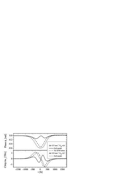
Fig. 4: Numerical simulations showing the FW phase and chirp after propagation in 50 mm BBO with a high fluence $\Phi_{1,\rm in}=272~{}{\rm mJ/cm^{2}}$ resulting in $N_{\rm eff,c}=8.4$. Input: $I_{1,\rm in}=400~{}{\rm GW/cm^{2}}$ and $T_{1,\rm in}=600$ fs FWHM.

We can conclude that $N_{\rm eff,c}$ deviates quite strongly from unity when the fluence (and thus the soliton numbers) is large. However, for $\Phi_{1,\rm in}\lesssim\Phi_{c}$, $N_{\rm eff,c}=1$ can be used as a safe estimate of the transition point.

B Scaling laws for compression parameters

We proceed to investigate how the soliton compressor behaves when compression is successful. We seek to find general scaling laws that can tell us at what position $z_{\rm opt}$ in the crystal the pulse reaches its optimal single-spike compressed state – i.e., with maximum intensity and minimum duration – and to check its duration, compression factor, and quality.

For soliton compression in the NLSE Mollenauer et al. [12] first studied the compression for $1<N_{\rm Kerr}<15$. Based on this Dianov et al. [14] showed the following empirical scaling law for the optimal compression length

$$\frac{z_{\rm opt}}{z_{0}}=\frac{0.32}{N_{\rm Kerr}}+\frac{1.1}{N_{\rm Kerr}^{2}},\quad 10<N_{\rm Kerr}<50,$$ (16)

where $z_{0}=\tfrac{\pi}{2}L_{\rm D,1}$ is the soliton length [10]. Also based on Ref. [12], Tomlinson et al. [13] reported the empirical scaling law for the compression factor $f_{c}\equiv T_{1,\rm in}/T_{1,\rm opt}$

$$f_{c} =4.1N_{\rm Kerr},\quad 1\ll N_{\rm Kerr}<50.$$ (17)

The validity range was reported in Ref. [14]. Finally, the pulse quality is defined as the fluence in a sech²-fit to the central spike relative to the input fluence $Q_{c}\equiv\Phi_{1,\rm sech-fit}/\Phi_{1,\rm in}$, which is equivalent to taking $Q_{c}=I_{1}/I_{1,\rm in}f_{c}$. Thus, we should expect that $Q_{c}\propto 1/f_{c}$ [11]. As we will now show, the cascaded quadratic soliton compressor follows nicely these scaling laws when $N_{\rm Kerr}$ is replaced by $N_{\rm eff}$. This holds as long as we are in the stationary regime, i.e., when the NLSE-like model Eq. (9) is a good approximation to the system and when GVM effects are small.

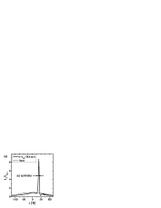
Fig. 5: Selected simulations of clean compressed pulses at the optimal compression length. (a) $\Delta k=50~{}{\rm mm^{-1}}$, $T_{1,\rm in}=200$ fs FWHM and $I_{1,\rm in}=59~{}{\rm GW/cm^{2}}$ ($N_{\rm eff}=8$) resulting in a 6.0 fs pulse ($f_{c}=33$) with $Q_{c}=0.26$. (b) $\Delta k=55~{}{\rm mm^{-1}}$, $T_{1,\rm in}=2000$ fs FWHM and $I_{1,\rm in}=26.7~{}{\rm GW/cm^{2}}$ ($N_{\rm eff}=50$) resulting in a 7.6 fs pulse ($f_{c}=264$) with $Q_{c}=0.06$.

We performed a wide range of simulations using sech-shaped un-chirped input pulses with parameters ranging from $T_{1,\rm in}=50-2000$ fs and $I_{1,\rm in}=10-400~{}{\rm GW/cm^{2}}$. The simulations used in the following resulted in cleanly compressed pulses as demonstrated in Fig. 5. It is worth to stress that the depletion of the FW due to conversion into SH was quite low in all cases ($<3\%$ in the stationary regime) due to the large values of phase mismatch $40<\Delta k<120$ accessible in the compression window. Some selected compression examples are given in Fig. 5: (a) shows a typical case with a 200 fs input, where we have optimized the phase mismatch and the input intensity to give a 6.0 fs compressed pulse. This implies a compression ratio of $f_{c}=33$ and the pulse quality is $Q_{c}=0.26$. The remaining pulse energy resides in the unwanted pedestal as well as in the SH (2.3% conversion occurred). As a more extreme case, (b) shows a 2 ps long pulse compressed to a clean 8.3 fs pulse, implying an impressive $f_{c}=264$. A lot of the energy remains in the pedestal (only 0.5% is converted to the SH), and the pulse quality is merely $Q_{c}=0.06$. This is typical of large compression ratios. Note the difference in $z_{\rm opt}$; $z_{\rm opt}=342~{}$mm in Fig. 5(b) is long, but may be realized using multiple crystals.

Fig. 6: Results of numerical simulations showing the optimum compression parameters vs. $N_{\rm eff}$ in log-log plots for (a) the compression length $z_{\rm opt}/z_{0}$, (b) the compression factor $f_{c}$ and (c) the compression quality $Q_{c}$. The simulations marked with round symbols resulted in a clean compressed pulse, while the triangles resulted in less clean pulses. The four black triangles gradually enter the nonstationary regime. The solid lines are fits to the clean data [Eqs. (18)-(20)], while the dotted lines are the scaling laws (16) and (17).

In Fig. 6(a) we show $z_{\rm opt}/z_{0}$ as function of the effective soliton number $N_{\rm eff}$. The data follow the scaling law (16) – with $N_{\rm Kerr}$ is replaced by $N_{\rm eff}$ – quite well, but there are deviations for small $N_{\rm eff}$. This is due to the $N^{-2}$ term in Eq. (16), so an improved fit gave

$$\frac{z_{\rm opt}}{z_{0}}=\frac{0.44}{N_{\rm eff}}+\frac{2.56}{N_{\rm eff}^{3}}-0.002.$$ (18)

We have also included data points where the compressed pulses were less clean (either having trailing or leading oscillations, or being somewhat asymmetric). As the plot indicates they start kicking in when $N_{\rm eff}>10$, which can be explained by increased XPM contributions as well as increased influence of the GVM induced Raman-like perturbation. Nonetheless, these less clean data still follow the scaling law (18) closely. An exception is when the nonstationary regime is close: We included four data points (black symbols), which have the same parameters as Fig. 5(a) and where $\Delta k$ is gradually decreased so the final data point is in the nonstationary regime. These data points start to deviate from the scaling laws because the compressed pulses experience more strongly the GVM induced Raman-like effects.

In Fig. 6(b) we plot the compression factor $f_{c}$ as function of $N_{\rm eff}$. Again the scaling law (17) holds well except for small $N_{\rm eff}$. A linear fit to the clean data gave the following scaling law valid also for small $N_{\rm eff}$

$$f_{c}=4.7(N_{\rm eff}-0.86).$$ (19)

The less clean data also follow the scaling law (19) quite well, but the data points approaching the nonstationary regime (black triangles) very quickly separate out. Thus, $f_{c}$ is very sensitive to the effects of the GVM induced Raman-like effects in the nonstationary regime.

As the last dimensionless parameter, we show in Fig. 6(c) the pulse compression quality $Q_{c}$ as a function of $N_{\rm eff}$. The data roughly follow a rational function

$$Q_{c}=[0.24(N_{\rm eff}-1)^{1.11}+1]^{-1}.$$ (20)

The exponent 1.11 deviates from unity due to the behaviour of $Q_{c}$ for small $N_{\rm eff}$. However, for large $N_{\rm eff}$ we find $Q_{c}\propto f_{c}^{-1}$, as predicted.

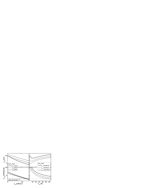
Fig. 7: The optimal compressor length and the expected compressed pulse duration in a BBO for $\lambda_{1}=1064$ nm and $\Delta k=50~{}{\rm mm^{-1}}$ with (a) $T_{1,\rm in}$ fixed; (b) $I_{1,\rm in}$ fixed.

As a more concrete example Fig. 7 shows the compressor length one should choose for optimal compression $z_{\rm opt}$, together with the expected compressed pulse duration. These were calculated from Eqs. (18) and (19) for $\Delta k=50~{}{\rm mm^{-1}}$. Single-cycle pulses are available for $I_{1,\rm in}>200~{}{\rm GW/cm^{2}}$ with realistic compressor lengths around $5-20$ mm.

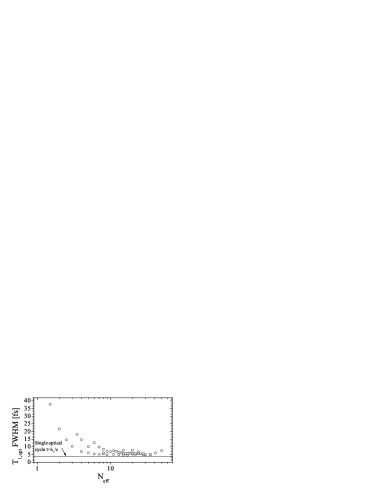
Fig. 8: The duration of the compressed pulse vs. $N_{\rm eff}$ in a log plot. The data are from the same simulations as in Fig. 6, but only those with $\Delta k=55~{}{\rm mm^{-1}}$ are shown.

Finally, Fig. 8 summarizes output pulse duration vs. $N_{\rm eff}$, providing a sense of the possible pulse compression in BBO at $\lambda_{1}=1064$ nm. The lowest value observed was 4.7 fs FWHM, corresponding to 1.3 optical cycles. Single-cycle pulses were not observed, most likely due to GVM-induced Raman effects and Kerr XPM effects.

4 Conclusions

In summary, we find that the effective soliton number $N_{\rm eff}=\sqrt{N_{\rm SHG}^{2}-N_{\rm Kerr}^{2}}$ is the proper dimensionless quantity for describing soliton compression using cascaded quadratic nonlinearities in the stationary regime. Soliton compression generally only occurs when $N_{\rm eff}>1$, and this in turn requires that the quadratic nonlinearity dominates over the cubic nonlinearity. In this balance, material and input pulse parameters such as the phase mismatch, the input pulse intensity and duration play a crucial role. When the pulse energy is large $N_{\rm eff}>1$ is no longer a sufficient demand. We attributed this to Kerr XPM effects, and we found an empirical scaling law relating $N_{\rm eff,c}$ to the input fluence.

We showed through a large number of realistic numerical simulations of a BBO crystal that the system clearly obeys dimensionless scaling laws dictating the optimal compression propagation distance, the pulse compression factor and quality. These scaling laws were expressed through the effective soliton number $N_{\rm eff}$, and are very similar to the ones observed in the NLSE. The scaling laws are general and hold also for other materials and wavelengths, and will serve as a crucial tool to determine input pulse peak intensity and duration as well as phase-matching conditions and optimal crystal lengths.

Besides the requirement of a strong quadratic nonlinearity, avoiding the nonstationary regime, where GVM-effects are strong, is another obstacle to observe the desired compression in the considered system. While compression may still occur, the final pulse is too distorted to be of any use due to GVM induced Raman-like effects. This is particularly a problem for short pulses, high intensity pulses, and in materials with a weak quadratic nonlinearity and/or large GVM. In this paper we considered the stationary regime, where this effect is negligible and stress that the scaling laws for compression hold only in this regime. In subsequent publications we will study the GVM effects in more detail, and show that the cascaded quadratic nonlinearity induces a nonlocal response on the FW, and that in presence of GVM this response becomes Raman-like [16]. Moreover, in the nonstationary regime the response function is no longer localized, which has severe implications on the compressed pulse.

Let us finally touch on the exciting prospect of the cascaded quadratic soliton compressor in a wave-guiding configuration. As mentioned, GVM effects are detrimental to the compression performance, and these become even more pronounced for shorter input wavelengths such as 800 nm because GVM is much stronger. However, in a photonic crystal fiber (PCF) wave-guiding effects can dramatically alter the dispersion, and in particular it was shown that for SHG it is possible to achieve zero GVM [24]. Moreover, in a PCF the mode areas are very small (roughly a few $\mu{\rm m^{2}}$ is possible) so very high peak intensities are possible even with very low pulse energies. This will allow achievement of low-energy clean compressed pulses, once issues with quadratic nonlinear response of optical fibers have been resolved.

5 Acknowledgments

M.B. was supported by The Danish Natural Science Research Council Grant 21-04-0506. J.M. and F.W.W. were supported by NSF Grants PHY-0099564 and ECS-0217958. O. Bang is acknowledged for discussions.

Appendix A The cubic nonlinear response

We here show how a cubic nonlinearity is included in the model. The cubic nonlinear polarization response is

$$\mathbf{P}_{\rm NL}^{(3)}=\varepsilon_{0}\iiint_{-\infty}^{\infty}dt_{1}dt_{2}dt_{3}\\ \times\underline{\underline{\chi}}^{(3)}(t-t_{1},t-t_{2},t-t_{3})\vdots\mathbf{E}(t_{1})\mathbf{E}(t_{2})\mathbf{E}(t_{3}),$$ (21)

$\underline{\underline{\chi}}^{(3)}$ is a rank 4 tensor describing the cubic nonlinear response of the material, which we let take the functional form $\underline{\underline{\chi}}^{(3)}(t_{1},t_{2},t_{3})=\underline{\underline{\chi}}^{(3)}R(t_{1})\delta(t_{2})\delta(t_{3})$, where $R(t)$ is the normalized material Kerr response function. In arriving at Eqs. (1) we then assumed the waves monochromatic and polarized along arbitrary directions $\mathbf{E}(t)={\rm Re}[{\mathbf{x}}_{1}E_{1}(t)e^{-i\omega_{1}t}+{\mathbf{x}}_{2}E_{2}(t)e^{-i\omega_{2}t}]$, where ${\mathbf{x}}_{j}$ is the unit polarization vector. In SHG the FW and SH waves are either all polarized along the same direction (Type 0), or the two FW are polarized along the same direction but orthogonal to the SH (Type I), or finally the two FW photons could be polarized orthogonally to each other while the SH is parallel with one of the FW photons (Type II) [19]. The propagation equations presented here are valid for Type 0 and I, since the FW photons are considered degenerate. We assume an isotropic cubic Kerr nonlinearity, for which the only nonzero tensor components of $\underline{\underline{\chi}}^{(3)}$ are $\chi^{(3)}_{xxyy}=\chi^{(3)}_{xyyx}=\chi^{(3)}_{xyxy}=\chi^{(3)}_{xxxx}/3$ [11]. This means that the XPM coefficient in Eq. (1a) is $B=2$ for Type 0 SHG, and $B=2/3$ for Type I SHG. We now divide the material Kerr response into an electronic response and a vibrational Raman response $R(t)=(1-f_{R})\delta(t)+f_{R}h_{R}(t)$ [10], where $f_{R}$ is the fractional contribution of the vibrational Raman response. The first part describes the electronic response, which can be considered instantaneous, resulting in the cubic SPM and XPM terms in Eqs. (1). The vibrational Raman response for a general 3-wave mixing process with two different frequencies is [25]

$$\mathcal{R}_{j}(\tau)\equiv\hat{S}_{j}\int_{-\infty}^{\infty}dsh_{R}(s)\\ \times\Big{\{}E_{j}(\tau)\left[|E_{j}(\tau-s)|^{2}+\tfrac{1}{2}B|E_{m}(\tau-s)|^{2}\right]\\ +\tfrac{1}{2}BE_{j}(\tau-s)E_{m}^{*}(\tau-s)e^{i(\omega_{j}-\omega_{m})s}E_{m}(\tau)\Big{\}},$$ (22)

where $j=1,2$ and $m=3-j$, and only terms that are phase matched are included [25]. This Raman response is governed by the gain function $h_{R}$. For SHG, the integral over the term containing $e^{i(\omega_{j}-\omega_{m})s}$ is vanishing since it implies evaluation of $h_{R}$ is evaluated at frequency offset $|\omega_{j}-\omega_{m}|=\omega_{1}$ much larger than the typical spectral width of $h_{R}$ (in the THz range). Therefore, for SHG only the term $E_{j}(\tau)\left[|E_{j}(\tau-s)|^{2}+\tfrac{1}{2}B|E_{m}(\tau-s)|^{2}\right]$ remains, and the generalized coupled equations (1) become

$$\hat{\mathcal{L}}_{1}E_{1}+\kappa_{\rm SHG,1}^{E}\hat{S}_{1}E_{1}^{*}E_{2}e^{i\Delta kz}$$ (23a)

$$+\kappa_{\rm Kerr,1}^{E}\hat{S}_{1}E_{1}\Bigg{\{}(1-f_{R})\left(|E_{1}|^{2}+B|E_{2}|^{2}\right)$$

$$+f_{R}\int_{-\infty}^{\infty}dsh_{R}(s)\left[|E_{1}(\tau-s)|^{2}+\tfrac{1}{2}B|E_{2}(\tau-s)|^{2}\right]\Bigg{\}}=0,$$

$$\hat{\mathcal{L}}_{2}E_{2}+\kappa_{\rm SHG,2}^{E}\hat{S}_{2}E_{1}^{2}e^{-i\Delta kz}$$ (23b)

$$+\kappa_{\rm Kerr,2}^{E}\hat{S}_{2}E_{2}\Bigg{\{}(1-f_{R})\left(|E_{2}|^{2}+B|E_{1}|^{2}\right)$$

$$+f_{R}\int_{-\infty}^{\infty}dsh_{R}(s)\left[|E_{1}(\tau-s)|^{2}+\tfrac{1}{2}B|E_{2}(\tau-s)|^{2}\right]\Bigg{\}}=0.$$

Finally, the Raman overlap integral has an approximate form for short, but not extremely short, pulses

$$f_{R}\mathcal{R}_{j}(\tau)\simeq f_{R}\hat{S}_{j}E_{j}(\tau)\left[|E_{j}(\tau)|^{2}+\tfrac{1}{2}B|E_{m}(\tau)|^{2}\right]\\ -\tau_{R}\frac{\partial}{\partial\tau}\left[|E_{j}(\tau)|^{2}+\tfrac{1}{2}B|E_{m}(\tau)|^{2}\right],$$ (24)

where we have used that $\int_{-\infty}^{\infty}dth_{R}(t)=1$, and defined the well-known Raman response time $\tau_{R}\equiv f_{R}\int_{-\infty}^{\infty}dt\,th_{R}(t)$. Eq. (24) is related to intra- and inter-pulse Raman scattering (IIRS), and Eqs. (23) become

$$\hat{\mathcal{L}}_{1}E_{1} +\kappa_{{\rm SHG},1}^{E}\hat{S}_{1}E_{1}^{*}E_{2}e^{i\Delta kz}$$ (25a)

$$+\kappa_{{\rm Kerr},1}^{E}\Big{\{}\hat{S}_{1}E_{1}\left[|E_{1}|^{2}+B(1-\tfrac{1}{2}f_{R})|E_{2}|^{2}\right]$$

$$\phantom{+\kappa_{{\rm Kerr},1}^{E}\Big{\{}}-\tau_{R}E_{1}\frac{\partial}{\partial\tau}\left(|E_{1}|^{2}+\tfrac{1}{2}B|E_{2}|^{2}\right)\Big{\}}=0,$$

$$\hat{\mathcal{L}}_{2}E_{2} +\kappa_{{\rm SHG},2}^{E}\hat{S}_{2}E_{1}^{2}e^{-i\Delta kz}$$ (25b)

$$+\kappa_{{\rm Kerr},2}^{E}\Big{\{}\hat{S}_{2}E_{2}\left[|E_{2}|^{2}+B(1-\tfrac{1}{2}f_{R})|E_{1}|^{2}\right]$$

$$\phantom{+\kappa_{{\rm Kerr},2}^{E}\Big{\{}}-\tau_{R}E_{2}\frac{\partial}{\partial\tau}\left(|E_{1}|^{2}+\tfrac{1}{2}B|E_{2}|^{2}\right)\Big{\}}=0.$$

Here we have neglected the 2nd order derivatives from applying self-steepening to the IIRS term in Eq. (24).

Appendix B Extending the propagation equations to the SEWA regime

Here we discuss the difference between the slowly varying envelope approximation (SVEA) and the SEWA propagation equations. SEWA [17] is a general spatio-temporal model that describes spatio-temporal pulse propagation down to single-cycle pulse durations. It was recently derived for SHG by Moses and Wise [18]. SEWA does not pose any direct constriction on the pulse bandwidth, whereas the extended SVEA (with steepening terms and the general Raman convolution response) holds for [26] $\Delta\omega/\omega<1/3$. Neglecting transverse spatial terms, the only term the SHG extended SVEA model does not include is related to the dispersion of the SH, since due to GVM the SH dispersion operator (3) must be replaced by the following effective operator [18] $\hat{\mathcal{D}}_{2,{\rm eff}}\equiv\hat{\mathcal{D}}_{2}+\hat{S}_{2}^{-1}\frac{d_{12}^{2}}{2k_{2}}\frac{\partial^{2}}{\partial\tau^{2}}$. Imposing the scalings $z^{\prime}=z/L_{\rm D,1}$ and $\tau^{\prime}=\tau/T_{1,\rm in}$, the dimensionless operator becomes

$$\hat{\mathcal{D}}^{\prime}_{2,{\rm eff}} \equiv\hat{\mathcal{D}}_{2}^{\prime}+\hat{S}_{2}^{\prime-1}\frac{\nu}{2}\frac{\partial^{2}}{\partial\tau^{\prime 2}},$$ (26)

where the dimensionless factor $\nu\equiv cd_{12}^{2}/\omega_{2}n_{2}|k^{(2)}_{1}|$. Expanding the inverse steepening operator $\hat{S}_{2}^{\prime-1}=\sum_{m=0}^{\infty}\left(\frac{-is^{\prime}}{2}\right)^{m}\frac{\partial^{m}}{\partial\tau^{\prime m}},$ we get

$$\hat{\mathcal{D}}^{\prime}_{2,{\rm eff}}=\sum_{m=2}^{\infty}i^{m}\left[\delta_{2}^{(m)}+\frac{\nu}{2}\left(\frac{s^{\prime}}{2}\right)^{m-2}\right]\frac{\partial^{m}}{\partial\tau^{\prime m}}.$$ (27)

In the SEWA there is no restriction on the pulse bandwidth so single-cycle temporal resolution is achieved. However, since we consider SHG we should be careful. One assumption made when deriving Eqs. (1) is namely that the spectra of the FW and SH do not overlap (substantially). This assumption allows us to separate the fields as shown in App. A. We chose $\Delta\omega/\omega_{j}=0.7$. This gives some overlap between the FW and SH spectra, but we always made sure that the spectral components in the overlapping regions were negligible.

Appendix C BBO

We use a $\beta$-${\rm BaB_{2}O_{4}}$ (beta-barium-borate, BBO) nonlinear crystal, where collinear Type I SHG is possible through the interaction ${\rm oo\rightarrow e}$, i.e. the FW photons are ordinarily polarized, while the generated SH photon is extraordinarily polarized. BBO is a uni-axial crystal where phase matching can be achieved by birefringent phase matching by changing the angle $\theta$ between the FW input and the optical $z$-axis of the crystal. $d_{\rm eff}$ also changes with $\theta$, and is on average 2.22 pm/V in the area in which we are interested in. The dispersion is calculated from the Sellmeier equations [19]. Note in this connection that the analytical transition to compression $N_{\rm eff,c}$, as calculated from Eq. (13), is on implicit form.

BBO is an excellent nonlinear medium for the current purpose because it has a decent quadratic nonlinear strength, and perhaps more important, it has a small GVM at NIR wavelengths, which is the major reason for using BBO instead of, e.g., periodically poled LiNbO₃ for these wavelengths. BBO also has a very low cubic nonlinear refractive index. As we noted from Eq. (10) the balance between these is crucial. BBO also has a very low two-photon absorption coefficient (except in the ultra-violet part of the spectrum [27]), justifying the approximation made in the derivation of Eqs. (5).

In the literature several values for the nonlinear refractive index have been reported. We chose to use $n_{{\rm Kerr},1}^{I}=3.65\pm 0.6\cdot 10^{-20}~{}{\rm m^{2}/W}$ reported in Ref. [28] mainly because the measurements are done at phase-matching angles close to ours and also used fs pulses, but also because this value in the past has given the best agreement with experimental observations.

References

- [1] R. DeSalvo, D. Hagan, M. Sheik-Bahae, G. Stegeman, E. W. Van Stryland, and H. Vanherzeele, “Self-focusing and self-defocusing by cascaded second-order effects in KTP,” Opt. Lett. 17, 28–30 (1992).
- [2] G. I. Stegeman, M. Sheik-Bahae, E. Van Stryland, and G. Assanto, “Large nonlinear phase shifts in second-order nonlinear-optical processes,” Opt. Lett. 18, 13–15 (1993).
- [3] C. R. Menyuk, R. Schiek, and L. Torner, “Solitary waves due to cascading,” J. Opt. Soc. Am. B 11, 2434–2443 (1994).
- [4] X. Liu, L. Qian, and F. W. Wise, “High-energy pulse compression by use of negative phase shifts produced by the cascaded nonlinearity,” Opt. Lett. 24, 1777–1779 (1999).
- [5] S. Ashihara, J. Nishina, T. Shimura, and K. Kuroda, “Soliton compression of femtosecond pulses in quadratic media,” J. Opt. Soc. Am. B 19, 2505–2510 (2002).
- [6] S. Ashihara, T. Shimura, K. Kuroda, N. E. Yu, S. Kurimura, K. Kitamura, M. Cha, and T. Taira, “Optical pulse compression using cascaded quadratic nonlinearities in periodically poled lithium niobate,” Appl. Phys. Lett. 84, 1055–1057 (2004).
- [7] X. Zeng, S. Ashihara, N. Fujioka, T. Shimura, and K. Kuroda, “Adiabatic compression of quadratic temporal solitons in aperiodic quasi-phase-matching gratings,” Opt. Express 14, 9358–9370 (2006).
- [8] J. Moses and F. W. Wise, “Soliton compression in quadratic media: high-energy few-cycle pulses with a frequency-doubling crystal,” Opt. Lett. 31, 1881–1883 (2006).
- [9] G. Xie, D. Zhang, L. Qian, H. Zhu, and D. Tang, “Multi-stage pulse compression by use of cascaded quadratic nonlinearity,” Opt. Commun. 273, 207–213 (2007).
- [10] G. P. Agrawal, Nonlinear fiber optics, 3 ed. (Academic Press, London, 2001).
- [11] G. P. Agrawal, Applications of nonlinear fiber optics (Academic Press, London, 2001).
- [12] L. F. Mollenauer, R. H. Stolen, J. P. Gordon, and W. J. Tomlinson, “Extreme picosecond pulse narrowing by means of soliton effect in single-mode optical fibers,” Opt. Lett. 8, 289–291 (1983).
- [13] W. J. Tomlinson, R. H. Stolen, and C. V. Shank, “Compression of optical pulses chirped by self-phase modulation in fibers,” J. Opt. Soc. Am. B 1, 139–149 (1984).
- [14] E. M. Dianov, Z. S. Nikonova, A. M. Prokhorov, and V. N. Serkin, “Optimal compression of multi-soliton pulses in optical fibers,” Sov. Tech. Phys. Lett. 12, 311–313 (1986), [Pis’ma Zh. Tekh. Fiz. 12, 756–760 (1986)].
- [15] F. Ö. Ilday, K. Beckwitt, Y.-F. Chen, H. Lim, and F. W. Wise, “Controllable Raman-like nonlinearities from nonstationary, cascaded quadratic processes,” J. Opt. Soc. Am. B 21, 376–383 (2004).
- [16] M. Bache, O. Bang, J. Moses, and F. W. Wise, “Nonlocal explanation of stationary and nonstationary regimes in cascaded soliton pulse compression,” Opt. Lett. 32, 2490–2492 (2007), arXiv:0706.1933.
- [17] T. Brabec and F. Krausz, “Nonlinear Optical Pulse Propagation in the Single-Cycle Regime,” Phys. Rev. Lett. 78, 3282–3285 (1997).
- [18] J. Moses and F. W. Wise, “Controllable Self-Steepening of Ultrashort Pulses in Quadratic Nonlinear Media,” Phys. Rev. Lett. 97, 073903 (2006), see also arXiv:physics/0604170.
- [19] V. Dmitriev, G. Gurzadyan, and D. Nikogosyan, Handbook of Nonlinear Optical Crystals, Vol. 64 of Springer Series in Optical Sciences (Springer, Berlin, 1999).
- [20] J. Moses, E. Alhammali, J. M. Eichenholz, and F. W. Wise, “Efficient High-Energy Femtosecond Pulse Compression in Quadratic Media with Flattop Beams,” in press (2007).
- [21] J. M. Dudley, G. Genty, and S. Coen, “Supercontinuum generation in photonic crystal fiber,” Rev. Mod. Phys. 78, 1135–1184 (2006).
- [22] C.-M. Chen and P. L. Kelley, “Nonlinear pulse compression in optical fibers: scaling laws and numerical analysis,” J. Opt. Soc. Am. B 19, 1961–1967 (2002).
- [23] J. Moses, B. A. Malomed, and F. W. Wise, “Self-Steepening of Ultrashort Optical Pulses without Self-Phase Modulation,” in press (2007).
- [24] M. Bache, H. Nielsen, J. Lægsgaard, and O. Bang, “Tuning quadratic nonlinear photonic crystal fibers for zero group-velocity mismatch,” Opt. Lett. 31, 1612–1614 (2006), arXiv:physics/0511244.
- [25] S. Kumar, A. Selvarajan, and G. Anand, “Influence of Raman scattering on the cross phase modulation in optical fibers,” Opt. Commun. 102, 329–335 (1993).
- [26] K. J. Blow and D. Wood, “Theoretical description of transient stimulated Raman scattering in optical fibers,” IEEE J. Quant. Electr. 25, 2665–2673 (1989).
- [27] R. DeSalvo, A. A. Said, D. Hagan, E. W. Van Stryland, and M. Sheik-Bahae, “Infrared to ultraviolet measurements of two-photon absorption and n2 in wide bandgap solids,” IEEE J. Quant. Electr. 32, 1324–1333 (1996).
- [28] M. Sheik-Bahae and M. Ebrahimzadeh, “Measurements of nonlinear refraction in the second-order materials KTiOPO4, KNbO3, -BaB2O4 and LiB3O5,” Opt. Commun. 142, 294–298 (1997).