Multiple hits in wire chambers and other particle detectors.

Abstract

We propose an analysis of the dead time losses in counting imaging detectors such as MWPC which can resolve $k$ simultaneous hits, and analyze in more detail an $X-Y$ detector which has a third wire set which allows for the recognition of simultaneous impacts.

1 Introduction: the standard $X-Y$ detector.

A particle detector with an intrinsic $X-Y$ structure, such as a MWPC (see for example [2]) can be used as a pulse counting 2-D imaging detector. A specific pixel of the imaging detector shares a specific readout channel $x_{1}$ with other pixels, and shares another specific readout channel $y_{1}$ with other pixels, but in such a way that the combination of $x_{1}$ and $y_{1}$ are not shared by any other pixel. A detector with $n_{x}\times n_{y}$ pixels can hence be read out with $n_{x}+n_{y}$ channels. As long as there is a single hit on the detector, giving rise to a single $X$ and a single $Y$ channel being hit, the hit pixel can be reconstructed without ambiguity. As long as the signal development time of a single hit is small compared to the time between impacts, a time correlation of $X$ and $Y$ hits can associate the right $X$-hit with the right $Y$ hit, and within this time window, a single hit will be able to be resolved into a single pixel.

However, from the moment that two (or more) successive impacts on the detector cannot be resolved in time, we have two (or more) $X$-hits, say channels $x_{1}$ and $x_{2}$, and two (or more) $Y$-hits, say channels $y_{1}$ and $y_{2}$, and it is not clear whether the association should be $(x_{1},y_{1})$ and $(x_{2},y_{2})$ or whether the association should be $(x_{1},y_{2})$ and $(x_{2},y_{1})$ — if there is no other information, such as amplitude correlations, and the hits are similar. In other words, a double impact generates 4 possible pixel candidates, of which 2 are the correct ones, and 2 others are ”ghost” hits. Let us consider that the largest time which can separate the $X$ and the $Y$ signal of a single hit, equals $\tau$, which we call the coincidence time. The only way to associate unambiguously an $X$ hit to a $Y$ hit is that during the time $\tau$ before and during the time $\tau$ after the event, no other event occurs. The probability in a Poissonian stream with $n$ hits per second on average, that during a time $T$ no event occurs, equals

$$P(T,k=0)=\exp\left(-nT\right)$$ (1)

The condition for an event, occurring at $t=0$ to be acceptable (no ghosts), is that during the interval $t=-\tau$ to $t=0^{-}$, no event happens, and that during the interval $t=0^{+}$ to $t=\tau$, no event happens. These probabilities being independent for a Poisson stream (as the intervals are disjoint), the probability for this to be so equals $P(\tau,k=0)^{2}=\exp\left(-n2\tau\right)$. As such, the number of recorded hits (with no ambiguity) in an $X-Y$ detector equals:

$$m=n\exp\left(-2n\tau\right)$$ (2)

In other words, an $X-Y$ detector behaves as a paralyzable (see for instance, [1]) detector, but with twice the coincidence time $\tau$ as dead time.

Of course, there is also an intrinsic dead time for each $X$ wire itself, and each $Y$ wire itself, which can often be longer than the coincidence time window $\tau$. If we call this wire dead time, $\tau_{w}$, the time during which no two distinct hits on the same $X$ wire can be distinguished, this will also give rise to a dead time, in parallel with the coincidence dead time above. In order to estimate its importance, let us suppose that our detector is uniformly irradiated. This means that an $X$ wire has an average Poissonian flux of $N_{x}=\frac{n}{n_{x}}$. For a given event at time $t=0$, we don’t want its $X$ wire to be ”blinded” by an event preceding it, outside of the already considered coincidence window. The probability that no event occurs on the same $X$ wire in the time window starting a time $t=-\tau_{w}$ but stopping at $t=-\tau$, the start of the coincidence window, equals, using equation 1, $\exp\left(-N_{x}(\tau_{w}-\tau)\right)$. We can apply the same reasoning for the $Y$ wire, so the joint probability that no event occurs, nor on the hit $X$ wire, nor on the hit $Y$ wire, so that both the $X$ and the $Y$ wire are not ”blinded” before the actual coincidence window opens, equals:

$$P_{w}=\exp\left(-\frac{n}{n_{x}}(\tau_{w}-\tau)\right)\exp\left(-\frac{n}{n_{y}}(\tau_{w}-\tau)\right)$$ (3)

The overall relationship between the true flux $n$, and the observed flux $m$, in the case of a uniform, Poissonian illumination, is:

$$m=n\exp\left(-2n\tau\right)\exp\left(-\frac{n}{n_{x}}(\tau_{w}-\tau)\right)\exp\left(-\frac{n}{n_{y}}(\tau_{w}-\tau)\right)=n\exp\left(-n\tau_{t}\right)$$ (4)

where

$$\tau_{t}=\tau\left(2-\frac{1}{n_{x}}-\frac{1}{n_{y}}\right)+\tau_{w}\left(\frac{1}{n_{x}}+\frac{1}{n_{y}}\right)$$ (5)

As such, a standard $X-Y$ detector has a counting behaviour which is that of a paralyzable detector with dead time given by $\tau_{t}$. We also see that this dead time consists of the ”coincidence dead time” ($2\tau$) and has a contribution of the ”wire dead time” of the order of $2\tau_{w}/n_{x}$. So, the wire dead time is less important (under uniform irradiation) when we have $\tau_{w}/n_{x}\ll\tau$, which is often the case for large MWPC.

2 A third ”disambiguation” electrode grid.

An MWPC is often made by ”sandwiching” an anode wire plane between two cathode wire planes, or between a cathode wire plane and a solid conductor surface. One can make use of this degree of freedom to use one cathode plane and the anode plane as the $X-Y$ channels, and the second cathode as a third set of channels. In the case of a wire plane, one can imagine for instance a set of wires under 45 degrees with the $X-Y$ grid. This has been proposed by Lewis [5]. It is also possible to use a more symmetrical setup where the 3 wire planes (two cathode planes and one anode plane in the case of a MWPC, or 3 different readout directions on other types of detectors) make angles of 60 degrees with each other, giving rise to some hexagonal ’honeycomb’ structure. This idea has been implemented using multi-GEM detectors for X-ray imaging [6], and the same idea has also been proposed and experimented for Cherenkov photon detectors (where there are typically simultaneous hits), in [7]. In order to analyze the principle however, which we set out to do in this paper, the exact geometry doesn’t matter, as long as the topological relationships between the coordinates are the same.

Let us call this third set of channels, the $Z$ channels. To each possible hit corresponds, as before, an $x_{i}$ and a $y_{j}$, but now also a $z_{k}$ channel hit, and the interesting point is that not all combinations of $x$, $y$ and $z$ correspond to existing pixels. In other words, for a single hit, there is some redundancy in the information. This redundancy can be used to try to find out what are the correct, and what are the ”ghost” combinations of $x$ and $y$, when we have a multiple-hit event. One can easily establish that it is always possible to find a numbering scheme of the channels $X$, $Y$ and $Z$, such that, with a hit $(x,y)$, there corresponds a $Z$-hit given by $z=x+y$. It is herein that lies the possibility to distinguish potentially multiple hits: of a list of $X$ signals $\{x_{1},x_{2},...\}$, a list of $Y$ signals $\{y_{1},y_{2},...\}$ and a list of $Z$ signals $\{z_{1},z_{2},...\}$, not all combinations are possible and one can hope that only the correct combinations are allowed for.

2.1 Two simultaneous hits.

In fact, amongst two hits, the disambiguation is complete. Imagine the hits $\{x_{1},x_{2}\}$, $\{y_{1},y_{2}\}$ and $\{z_{1},z_{2}\}$ (where we don’t know of course the right numbering when we reconstruct them). The right hits are $(x_{1},y_{1},z_{1})$ and $(x_{2},y_{2},z_{2})$. This means that $z_{1}=x_{1}+y_{1}$ and $z_{2}=x_{2}+y_{2}$. The question is: are there other possibilities ? Let us assume that $x_{1}\neq x_{2}$, $y_{1}\neq y_{2}$ and $z_{1}\neq z_{2}$ for starters. Imagine that $(x_{1},y_{2},z_{1})$ is a solution too. This means that $z_{1}=x_{1}+y_{2}$, from which follows that $y_{1}=y_{2}$ what was against the starting hypothesis. A similar conclusion can be drawn for the case $(x_{1},y_{2},z_{2})$, and all other thinkable cases can be reduced to these two by permutations. On the other hand, imagine that $x_{1}=x_{2}$. In that case, both the $(x_{1},y_{1},z_{1})$ and $(x_{1},y_{2},z_{2})$ are the right solutions, and there are no others (no ghosts can be constructed).

So this means that two simultaneous hits can be recognized correctly with certainty. If we limit ourselves to this result, then we can calculate the relation between true counting rate and observed counting rate. An event will be lost, if there is more than one (other) event in the time frame that starts time $\tau$ before and ends time $\tau$ after it. The Poisson distribution is given by $P(k,\lambda)=\frac{\exp\left(-\lambda\right)\lambda^{k}}{k!}$, from which it follows that $P(k<u,\lambda)=\sum_{k=0}^{u-1}P(k,\lambda)=\frac{\Gamma(u,\lambda)}{\Gamma(u)}=Q(u,\lambda)$ with $Q$ the regularized incomplete gamma function (in [3], the incomplete gamma function $P(a,x)=1-Q(a,x)$ is introduced ; see also [4]). So the probability that an event gets accepted is equal to $P(k<2,2n\tau)=\Gamma(2,2n\tau)=e^{-2n\tau}(1+2n\tau)$, which is the probability that in the interval of length $2\tau$, centered onto the event under discussion (but without counting this event of course) there is one or no hits. As such, the observed counting rate will be:

$$m=ne^{-2n\tau}(1+2n\tau)$$ (6)

We see that (as far as coincidence dead time is concerned), a detector that can discriminate up to two simultaneous hits, does not exactly follow a paralysable or non-paralysable model, but does in fact, much better: there is no first order dead time!

$$m\simeq n-2\tau^{2}n^{3}+...$$ (7)

2.2 $k$ simultaneous hits.

Let us imagine for a moment that we have a detector that can discriminate, without any difficulty, up to $k$ simultaneous events. What’s the ”dead time” now ? For a Poisson distribution, in order for an event to be counted, we need to have less than $k$ events in an interval of $2\tau$ centered on an event to be counted. We will assume that the dead time is caused by the coincidence time window needed, and is not dominated by individual ”wire” dead times. By a similar reasoning as above, we will obtain that the observed counting rate will be:

$$m=nP(<k,2n\tau)=nQ(k,2n\tau)=ne^{-2n\tau}\sum_{u=0}^{k-1}\frac{(2n\tau)^{u}}{u!}$$ (8)

For $k=2$, we find the same expression as in equation 6. For $k=3$, we find:

$$m=ne^{-2n\tau}\left(1+2n\tau+2n^{2}\tau^{2}\right)$$ (9)

This is interesting, because we see that the last term neutralizes the significant correction term in equation 7. We now have for low rates:

$$m\simeq n-\frac{4\tau^{3}n^{4}}{3}+...$$ (10)

In figure 1, we show the relationship between a (normalized on $1/\tau$) incoming Poissonian flux and the (also normalized) counting rate of discriminated events for $k=1,2,3,4,5$. Often, the ”dead-time correction” (which is given by $1-m/n$) shouldn’t be too important if one wants to give quantitative credibility to an imaging detector, and at the ILL, we take as a definition of acceptable counting rate for a detector, the one where the dead time correction is equal to 10%. The ”dead time correction factor” $1-m/n$ is shown in figure 2. In our case, we find then that this counting rate $n_{10\%}$ is given by the solution of the following equation:

$$Q(k,2n_{10\%}\tau)=0.9$$ (11)

which leads to a solution using the inverse regularized gamma function (see [4]):

$$n_{10\%}=\frac{Q^{-1}(k,0.9)}{2\tau}$$ (12)

Of course, the 10% can be judged a bit too severe, and some prefer allowing for 20% correction, in which case we have:

$$n_{20\%}=\frac{Q^{-1}(k,0.8)}{2\tau}$$ (13)

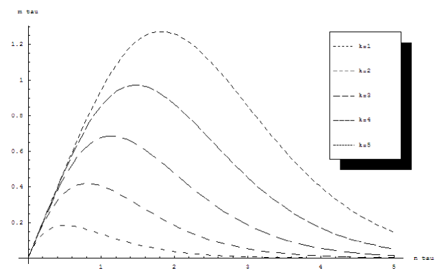
Figure 1: Observed counting rates as a function of incoming flux, when up to $k$ events can be discriminated in a time $\tau$.

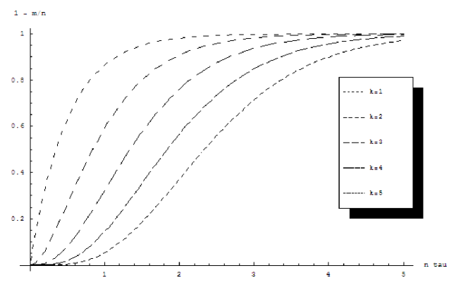
Figure 2: Dead time correction factor as a function of incoming flux, when up to $k$ events can be discriminated in a time $\tau$.

Solving these equations for the first 5 $k$-values, we find:

$k$	$2n_{10\%}\tau$	$2n_{20\%}\tau$
1	$0.105$	0.223
2	$0.531$	0.824
3	1.102	1.535
4	1.745	2.297
5	2.433	3.090

So, for a traditional wire chamber, we find that a 10% dead time correction is reached when the flux is 0.105 times $1/(2\tau)$; when the chamber can distinguish 2 simultaneous hits, this flux is 5 times greater. When the chamber can distinguish 3 simultaneous hits, this flux is 2 times greater again, etc… If we adhere to the definition of maximum flux at 20% dead time correction, being able to distinguish 2 simultaneous hits gives about 4 times higher counting rates and being able to distinguish 3 simultaneous hits adds a small factor 2 on top of this.

We hence see that the biggest gain in counting rate (as of our definition using a maximum dead time correction of 10% or 20%) occurs when we go from single-hit to double-hit identification, which can, as shown previously, be obtained by using a third grid.

2.3 How many hits can a third grid accept simultaneously ?

If there are more than two simultaneous hits, then a third electrode cannot guarantee that no ghost hit will be present. Let us consider the case of 3 simultaneous hits, and let us consider that $(x_{1},y_{2},z_{3})$ is a ghost hit. If there is a ghost hit, we can always permute indices to have the $X$ value be $x_{1}$ and the $Y$ value be $y_{2}$. In this case, the $Z$ value can only be $z_{3}$, as any other value would bring us back to the case of two hits and a ghost, which we demonstrated, is not possible. So the condition to have a ghost hit for a simultaneous impact of 3 hits is:

$$x_{1}+y_{2}=x_{3}+y_{3}$$ (14)

(or a similar condition for permuted indices). Nevertheless, most of the time when we have 3 hits the above condition will not be satisfied. In that case, the signals still allow for a non-ambiguous reconstruction of the 3 events. In order to find out in detail what percentage of possible $k$-hit events can be resolved one can take two roads: one is, for a specific setup, to have a Monte-Carlo simulation of $k$-hit events ; the other is to use some analytical estimations. In any case, the percentage of such resolved hits will depend also on the specific image that is projected onto the detector: we will assume uniform irradiation in our analysis.

2.3.1 Analytical estimation of resolution of $k$-hit events.

Imagine that we have a $k$-hit event. This means, a priori (we’ll come to that), that we have $k$ $X$ values, $k$ $Y$ values and $k$ $Z$ values. We will assume (which is, depending on the exact geometry of the detector, only approximately true), that each of the $n_{x}$ $X$ values are equally probable, that each of the $n_{y}$ $Y$ values are equally probable, and that each of the $n_{z}$ $Z$ values are equally probable. For each possible combination of an $X$ value (in the hit list), and a $Y$ value (also in the hit list), we can calculate the corresponding $Z$ value (using $z=x+y$). If this $Z$ value is in the list of $Z$ hits, we have to accept the hit. Of course, for the real hits, this will be the case. It is for the $k(k-1)$ wrong combinations of $X$ and $Y$ values $(x_{i},y_{j})$ that we shouldn’t, by coincidence, fall on a $Z$ value $z_{m}$ which is also present in the hit list. By a previous reasoning, we already know that this $z_{m}$ value cannot be the $Z$ value which goes with the correct event of the $X$ value $x_{i}$, or of the $Y$ value $y_{j}$, so the potential index $m$ cannot be $i$ or $j$. As such, there are $(k-2)$ possible $Z$ values which could, by coincidence, be equal to $x_{i}+y_{j}$. In order for our ghost couple $(x_{i},y_{j})$ to be rejected, none of these should be equal to $x_{i}+y_{j}$. Assuming (which is an approximation, but a reasonable one) that we can consider these $(k-2)$ values (out of $n_{z}$ possible) as being statistically independent, the probability for $x_{i}+y_{j}$ to be equal to one of them equals then $\frac{k-2}{n_{z}}$, so the probability not to have a ghost hit for $(x_{i},y_{j})$ equals $1-\frac{k-2}{n_{z}}$. There are $k(k-1)$ of these different combinations $(x_{i},y_{j})$ possible, so the probability (if, again, we consider all these potential coincidences as statistically independent, which is of course approximate but a reasonable hypothesis) that none of these combinations gives rise to a ghost hit (and hence, the $k$-hit event is totally identifiable), is then:

$$P_{good}^{0}=\left(1-\frac{k-2}{n_{w}}\right)^{k(k-1)}$$ (15)

In the above formula, we have put $n_{w}=n_{x}=n_{y}=n_{z}$ the number of channels, chosen to be equal for $X$, $Y$ and $Z$. What is clear is that when $n_{w}$ goes to infinity (infinitely many channels per coordinate), that all $k$-fold hits are resolvable. It is only due to a finite number of channels that 3 or more hits can potentially give rise to ghost hits.

There is a caveat, however. If we have $k$ hits and there is a finite number of channels, then there is also a finite probability that there are less than $k$ $X$-wires hit, or less than $k$ $Y$ wires hit or less than $k$ $Z$ wires hit because of the finite probability to hit the same wire twice.

In the appendix in subsection A.1, the number $Z^{l}_{k,n}$ is introduced, which gives us the number of different ways one can construct an ordered list of $k$ elements, of which each element is one of $n$ possible ones, and in which there are exactly $l$ different elements present. This corresponds to the number of ways one can distribute $k$ hits over $n$ different wires, and touch in all $l$ different wires. Under a uniform irradiation with ”distinguishable” hits, each of these different ways is equally probable, and hence the probability, if there are $k$ hits, to have $l$ wires hit, is given by:

$$P(l;k,n_{w})=\frac{Z_{k,n_{w}}^{l}}{n_{w}^{k}}$$ (16)

So a better approximation for the probability of being able to identify correctly a $k$-hit event, is to use formula 15 with the average value of $l$:

$$\langle l\rangle_{k}=\sum_{l=1}^{k}P(l;k,n_{w})l$$ (17)

to give:

$$P_{good}(k)=\left(1-\frac{\langle l\rangle_{k}-2}{n_{w}}\right)^{\langle l\rangle_{k}(\langle l\rangle_{k}-1)}$$ (18)

2.3.2 Monte Carlo estimation of resolution of $k$-hits

Let us consider a detector with 3 wire grids, at 120 degrees one from the other and 32 wires each, equally spaced. We delimit the ”useful” space as the hexagonal surface that is covered by the 3 different wire sets simultaneously, which consists of 768 pixels (out of the 1024 crossing points of each pair of $32\times 32$ wire planes). To each of these pixels correspond hence 3 numbers, $x_{i},y_{i},z_{i}=x_{i}+y_{i}$. A $k$-hit is formed by drawing independently $k$ natural numbers between 1 and 768 (corresponding to the pixels), and looking up what $x,y,z$ values they correspond to, to make up the lists of $X$, $Y$ and $Z$ hits. Next, all values of $(x_{i}+y_{j})_{i\neq j}$ are tested against all values of $z_{u}$ with $u\neq i,j$: these are the ghosts that cannot be rejected ; we count how many there are. We repeat this procedure a large number of times (number of trials $N$) and make then a histogram of the number of ghosts that each trial generated. Zero ghosts means that the event could be correctly reconstructed. The fraction of the number of zero ghosts $N_{0}(k)$ over $N$ is an estimator of the probability to be able to reconstruct a $k$-hit event.

For $N=10000$, we find:

$k$	1	2	3	4	5	6	7	8	9	10	11	12
$N_{0}(k)$	10000	10000	8639	5772	2780	918	215	41	7	1	0	0

If we compare that with our analytical estimation in equation 18 (multiplied with $N$), then we obtain:

$k$	1	2	3	4	5	6	7	8	9	10	11	12
$NP_{good}(k)$	10000	10018	8526	5336	2167	513	65	4	0	0	0	0

which gives quite good agreement especially for the lower $k$ values. For the higher $k$ values, there is an under-estimation of the number of correctly identified $k$-hits.

Repeating the experience with 128 wires per plane, we find, after 10000 trial events, for the Monte Carlo result:

$k$	1	2	3	4	5	6	7	8	9	10	11	12
$N_{0}(k)$	10000	10000	9612	8605	6820	4750	2701	1326	461	153	24	8

while the analytical estimation gives us:

$k$	1	2	3	4	5	6	7	8	9	10	11	12
$NP_{good}(k)$	10000	10001	9559	8356	6402	4123	2148	869	264	58	9	1

Again, one observes a relatively good performance for the lower $k$-values, and an underestimation of the number of correctly identified events at higher $k$ values.

2.4 Count rates, dead times, and the third coordinate.

Previously, we considered detectors which could, with 100% certainty, discriminate an event when there were no more than $k-1$ other events in a time slot $2\tau$ centered on our event, and which couldn’t handle, also with certainty, an event when there were $k$ or more events in the given time slot. The detector with a third coordinate however, has a different behavior: it can discriminate, with a certain probability $P_{good}(k)$, the case where there are $(k-1)$ events in the said time slot (on top of our event-under-test). This means that the relationship between incoming flux and observed, identified rate of hits is now given by:

$$m=n\sum_{k=1}^{\infty}P_{Pois}(k-1,2\tau n)P_{good}(k)$$ (19)

a sum which we can of course truncate to the first few terms given that as well the probability to have a $k$-hit as well as the probability to resolve it correctly, will drop fast for high $k$ values. As such, our analytical estimate can be used, given that its performance for relatively low $k$ values is adequate. Using equation 19, we can plot (figure 3) the observed (normalized) counting rate of identified events as a function of the incoming flux, for different numbers of wires per plane. The associated dead time correction is shown in figure 4. Calculating the incoming fluxes that give rise to a dead time correction of 10% or 20%, we find (normalized onto $2\tau$ as was the case in the fixed $k$ case):

Number of wires per plane	$n_{10\%}2\tau$	$n_{20\%}2\tau$
32	1.203	1.771
64	1.502	2.178
128	1.917	2.734
256	2.472	3.467

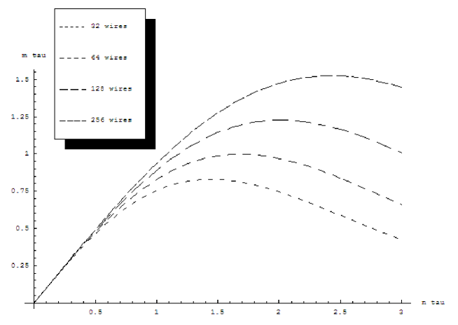
Figure 3: The observed (normalized) counting rate of identified hits as a function of the (normalized) incoming flux, using equation 19.

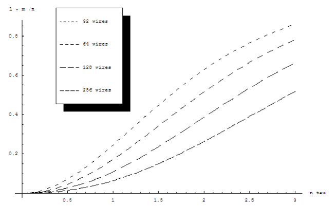
Figure 4: The dead time correction of identified hits as a function of the (normalized) incoming flux, using equation 19.

3 Conclusion.

In this paper we discussed the theoretical dead time correction occurring in detectors which need a certain time to recognize the correct positioning of an impact in the case that they can handle $k$ impacts simultaneously. We applied this to the specific case of a detector with an $X-Y-Z$ planar wire structure. It is established that in principle, such a detector (which has 50% more readout channels than a standard $X-Y$ detector) can accept incoming counting rates which are about 12 times (or more) larger than the standard $X-Y$ detector at 10% dead time correction. As such, the investment in 50% more channels can result potentially in 1200% higher counting rates. However, these results are only established in the case of a Poissonian, uniform irradiation.

We established a relatively simple analytical estimate of the dead time correction, and verified its applicability with a more detailed Monte Carlo simulation.

Appendix A Counting multi-hits.

A.1 Counting distinguishable hits.

Let us define a $k$-fold multiple hit event on a set of ”pixels” with $n$ possible ”positions” as an ordered series $\{x_{1},x_{2},...,x_{k}\}$, where $x_{i}$ takes its values out of the set $\{1,2,...n\}$. The point is of course that the $j$-th hit can be identical to the $i$-th hit, so this is the well-known problem of an ordered set with repetitions. The number of different such $k$-fold hit events is then given by the formula:

$$Z_{k,n}=n^{k}$$ (20)

where we introduced the symbol $Z_{k,n}$ to stand for the number of ordered sets of $k$ hits out of, each time, $n$ possibilities. Let us remind, for completeness, that, if we were not to allow repetitions (that is, we require the $k$ hits to be different), that the number of possibilities is the number of permutations:

$$P^{n}_{k}=\frac{n!}{(n-k)!}$$ (21)

We now want to find out, in the case of ordered sets with repetitions, what is the number of different $k$-fold hit events, in which there are exactly $l$ different values occurring in the series, where of course $l\leq k$ and $l\leq n$. Indeed, because of the possibility of repetitions, some of the $k$ different drawings can be identical, and we want to know how many different cells are finally hit by the $k$ hits. We will call this number: $Z_{k,n}^{l}$. We didn’t find any explicit reference to this number in the literature, but one can easily find a recursive definition for it. First, we consider special cases:

• The case $l=k$. We want all $k$ hit cells to be different. This is just drawing without repetition:

  $$Z_{k,n}^{k}=P^{n}_{k}=\frac{n!}{(n-k)!}$$ (22)

• The case $l=1$. All $k$ hits are identical. Clearly, there are exactly $n$ different ways to do so:

  $$Z_{k,n}^{1}=n$$ (23)

• The recurrence step. In order to compute $Z_{k,n}^{l}$, we consider that we have already $(k-1)$ hits, and we add the last hit. There are two possibilities: or there are already $l$ different elements hit in the $(k-1)$ first hits, in which case the $k$-th hit must be one of these $l$ elements ; or there were only $(l-1)$ different elements hit in the first $(k-1)$ hits, and hence the last hit must be a different hit, drawn from the $(n-l+1)$ remaining un-hit cells. As such, we obtain:

  $$Z_{k,n}^{l}=Z_{k-1,n}^{l}.l+Z_{k-1,n}^{l-1}.(n-l+1)$$ (24)

The two special cases and the recurrence relation define the function $Z_{k,n}^{l}$ completely: indeed, at each recurrence step, $k$ is diminished by 1, while $l$ remains, or is diminished by 1. So sooner or later, $k$ will reach the value of $l$, in which case the first special case is applicable, or $l$ will reach the value of $1$, in which case the second special case is applicable.

One should obtain that:

$$\sum_{l=1}^{k}Z_{k,n}^{l}=Z_{k,n}=n^{k}$$ (25)

Indeed, when summing over all possibilities of exactly $l$ different cells, we obtain of course all the possibilities of drawing $k$ hits out of $n$ possible cells. We didn’t succeed in obtaining an entirely closed form for the solution, but we did find solutions in closed form for small values of $l$ :

$$Z_{k,n}^{2} = \frac{\left(-2+2^{k}\right)\,\left(-1+n\right)\,n}{2}$$ (26)

$$Z_{k,n}^{3} = \frac{\left(27-27\,2^{1+k}+17\,3^{k}\right)\,\left(-2+n\right)\,\left(-1+n\right)\,n}{54}$$ (27)

$$Z_{k,n}^{4} = \frac{\left(-384+9\,2^{8+k}-2176\,3^{k}+555\,4^{k}\right)\left(n-3\right)\left(n-2\right)\left(n-1\right)n}{2304}$$ (28)

A.2 Counting indistinguishable hits.

Consider, for completeness, the case where the hits are indistinguishable in principle. In that case, the order of the hits in a $k$-hit event is unimportant. We can introduce a similar quantity to $Z_{k,n}^{l}$, namely, $K_{k,n}^{l}$, with the meaning of $l$ different cells being hit in a $k$-hit event out of $n$ possible different cells, but this time where the order is unimportant (though the multiplicity is). The total number of different (unordered) multisets with repetition with cardinality $k$ drawn out of $n$ possible values is known to be:

$$\langle\begin{array}[]{c}n\\ k\\ \end{array}\rangle=\left(\begin{array}[]{c}n+k-1\\ k\\ \end{array}\right)=\left(\begin{array}[]{c}n+k-1\\ n-1\\ \end{array}\right)$$ (29)

Here, $\left(\begin{array}[]{c}n\\ k\\ \end{array}\right)=C_{n}^{k}$ is the binomial coefficient.

If we consider $k$ unordered hits without repetition then we simply have the number of combinations, given by the binomial coefficient. From this, we can deduce that:

$$K_{k,n}^{k}=C_{n}^{k}$$ (30)

We can also deduce that:

$$\sum_{l=1}^{k}K_{k,n}^{l}=\langle\begin{array}[]{c}n\\ k\\ \end{array}\rangle$$ (31)

In order to derive a general expression for $K_{k,n}^{l}$, we consider the following ordering of the $k$ hits: the first $l$ cells are the cells which have distinct hits, and the last $k-l$ cells are the cells which have already been hit. The first $l$ cells (all different) can be chosen in $C_{n}^{l}$ different ways out of the $n$ existing cells. The last $k-l$ cells have to be all the unordered drawings with repetition out of the $l$ cells that have already been chosen in the first part: there are $\langle\begin{array}[]{c}l\\ k-l\\ \end{array}\rangle$ ways of doing this. So we conclude that:

$$K_{k,n}^{l}=C_{n}^{l}.C_{k-1}^{k-l}$$ (32)

and we have an explicit, closed-form expression for the unordered multisets of cardinality $k$, with exactly $l$ distinct elements, drawn out of $n$ possibilities.

Appendix B Dead times.

The classical models of paralyzable and non-paralysable detectors (see [1] for instance) are defined as follows: a non-paralyzable detector is ”blind” for a fixed time $\tau$ after an event is registered (no matter what happens during this time), and is sensitive again after this time. The relationship between the true rate $n$ and the observed rate $m$ is then given by:

$$n=\frac{m}{1-m\tau}$$ (33)

If the detector is ”far from saturation” (relatively few events are lost), then we can write:

$$m\simeq n(1-\tau n)$$ (34)

In the case of a paralyzable detector, the detector is ”blind” for at least a time $\tau$ after an event is registered, but each time there is a new (uncounted) event during the ”blind period”, the detector remains blind for a time $\tau$ after this event. In other words, the detector becomes ready again only if there is a time of ”silence” after an event of at least $\tau$. A detectable event must hence be preceded by a silence of at least $\tau$. We summarise the derivation given in [1], because it will be instructive for our own developments in this text. The probability, given an event at time $t=0$, to have the next event happening between time $t$ and time $t+dt$, equals, for a Poisson stream:

$$I_{1}(t)dt=n\exp(-nt)dt$$ (35)

The probability to have an event occurring after a ”silence” of at least time $\tau$ is then given by

$$\int_{t=\tau}^{\infty}I_{1}(t)dt=\exp(-n\tau)$$ (36)

This gives then:

$$m=n\exp(-n\tau)$$ (37)

If the detector is ”far from saturation”, then we can write also:

$$m\simeq n(1-\tau n)$$ (38)

so, far from saturation, there is no difference in behavior between a paralyzable and a non-paralyzable detector.

References

- [1] Glenn F. Knoll, Radiation Detection and Measurement (third edition) ©2000 John Wiley and Sons.
- [2] F. Sauli, Principles of Operation of Multiwire Proportional and Drift Chambers, CERN 77-09, 1977.
- [3] M. Abramowitz and I. A. Stegun, Handbook of Mathematical Functions, ©1965 Dover Publications.
- [4] http://functions.wolfram.com
- [5] R. Lewis, J. Synchrotron Rad. (1994) 1, 43-53.
- [6] S. Bachmann et al., Nucl. Instr. Meth. Phys. Res. A 478 (2002), 104-108.
- [7] F. Sauli, Nucl. Instr. Meth. Phys. Res. A 553 (2005) 18-24.