Can degenerate bound states occur in one dimensional quantum mechanics?

Abstract

We point out that bound states, degenerate in energy but differing in parity, may form in one dimensional quantum systems even if the potential is non-singular in any finite domain. Such potentials are necessarily unbounded from below at infinity and occur in several different contexts, such as in the study of localised states in brane-world scenarios. We describe how to construct large classes of such potentials and give explicit analytic expressions for the degenerate bound states. Some of these bound states occur above the potential maximum while some are below. Various unusual features of the bound states are described and after highlighting those that are ansatz independent, we suggest that it might be possible to observe such parity-paired degenerate bound states in specific mesoscopic systems.

The purpose of “no-go” theorems in physics is to delimit what is possible, and what is not, within a particular mathematical model of physical phenomena. Of course Nature is not obliged to respect our prejudices, so the assumptions used in proving such theorems should be well-motivated. Even then, some condition often gets slipped in, or in time forgotten, leading to confusion when counter-examples are found. In this Letter we discuss one such theorem and its possible physical consequences.

An often quoted result in quantum mechanics states that in one space dimension, potentials that are continuous and bounded from below cannot produce degenerate bound states. Elementary versions of the proof go as follows landau . Consider the stationary Schrodinger equation on the open line $-\infty<x<\infty$,

$$\psi^{{}^{\prime\prime}}+k^{2}(x)\psi=0\,,$$ (1)

with $k^{2}(x)\equiv E-V(x)$, and where we assume for convenience a symmetric potential, $V(x)=V(-x)$. As the equation is real we can, without loss of generality, discuss its real solutions. For two bound states $\psi_{1},\psi_{2}$ of the same energy, one deduces from (1) that the Wronskian

$$W\equiv\psi_{2}\psi_{1}^{{}^{\prime}}-\psi_{1}\psi_{2}^{{}^{\prime}}\,$$ (2)

is a constant, $W=C$. The constant $C$ can be evaluated at any point and for bound states the point at infinity is natural since the wavefunctions vanish there. If $C=0$ then (2) implies

$${\psi_{1}^{{}^{\prime}}\over\psi_{1}}={\psi_{2}^{{}^{\prime}}\over\psi_{2}}$$ (3)

and so we have $\psi_{1}\propto\psi_{2}$: the states are not independent, there is no degeneracy.

One way of avoiding the conclusion of the theorem was argued long ago loudon . The expression (3) is ill-defined at places where the wavefunction vanishes, and it was argued that if the potential was singular at a node of the wavefunctions then one could produce degenerate bound states cohen . These have been studied by a number of authors, and it has also been suggested that some of the singular potentials approximate certain physical situations in molecular chemistry pathak and elsewhere Wan . However, it should be noted that singular potentials by themselves do not guarantee degeneracy pathak ; Wan .

Let us suppose now that the potential is non-singular in any finite domain. Is the proof then complete? Not quite–there is still a loophole in the above argument. In order for the Wronskian in (2) to vanish at infinity for bound states we need to assume that the states have finite slopes at infinity. While this may seem a reasonable assumption, it is not necessarily true as we shall see below. The extra ingredient that is needed in the proof is that the potential be bounded from below messiah : then, if, asymptotically $k^{2}>0$, one has the usual continuum of scattering states , while the bound states exist if, asymptotically, $k^{2}<0$, i.e. the energy $E$ lies inside a potential well. A more involved reasoning messiah then shows that the bound states have the usual behaviour at infinity, with finite derivatives (for potentials that are finite but oscillatory at infinity one can have bound states in the continuum bic , but they have finite slopes).

A physical way of understanding the relationship between the diverging slope of a bound state and unbounded potentials is as follows: If the slope diverges, the state has diverging momentum and hence diverging mean kinetic energy. Therefore the mean potential energy of the state must be negative and divergent so as to get a total mean energy, $E$, that is finite. That is, the potential must be unbounded below.

Thus, it seems that if the potential is non-singular, then the only way to by-pass the theorem, and so produce degenerate bound states, is to study potentials that are unbounded from below at infinity. (Of course if one considers compact spaces, for example physics on a circle with periodic boundary conditions, then all states are localised and can be degenerate, see for example Wan ).

Bottomless potentials are neither uncommon nor necessarily pathological. For example the Coulomb potential is unbounded at the origin. Yet the hydrogen atom has a stable ground state, prevented from collapsing by quantum fluctuations, as is usually argued heuristically using the uncertainty principle. Potentials unbounded from below have also been studied in the context of non-Hermetian Hamiltonians bender which still produce real spectra because of a $PT$ symmetry. It has been shown that such systems may be mapped to a different Hermetian system mos although the mapping is known explicitly only in a few cases bus .

Unbounded potentials have also appeared in the context of localisation of fields on the brane in models with warped extra dimensions braneworld . In a recent study koleykar it was found that the following bottomless potential

$$V(x)=-(A_{1}\cosh^{2\nu}x+A_{2}\hskip 2.84544pt\mbox{sech}^{2}x)\,,$$ (4)

where $\nu>0$ and $A_{2}=\frac{\nu}{2}(\frac{\nu}{2}+1)$, led to opposite parity bound states with the same energy,

$$\psi_{1}(x)=\frac{\cos\left[\sqrt{A_{1}}\hskip 2.84544pt\int(\cosh x)^{\nu}dx\right]}{(\cosh x)^{\frac{\nu}{2}}}$$ (5)

$$\psi_{2}(x)=\frac{\sin\left[\sqrt{A_{1}}\hskip 2.84544pt\int(\cosh x)^{\nu}dx\right]}{(\cosh x)^{\frac{\nu}{2}}}$$ (6)

(see also choho where degenerate bound states were studied for a special case of (4)). Figure 1 shows the potential, the degenerate even and odd parity states and the energy. By tuning the parameter $A_{1}$ (with fixed $\nu$) one can have bound states inside or outside the well. Notice that in this example, while the wavefunctions vanish at infinity, their slope does not, and thus $C\neq 0$ in (2). Potentials of such shape are sometimes called “volcano” potentials and various aspects of such systems, such as the perturbation series and resonances, have been studied volcano .

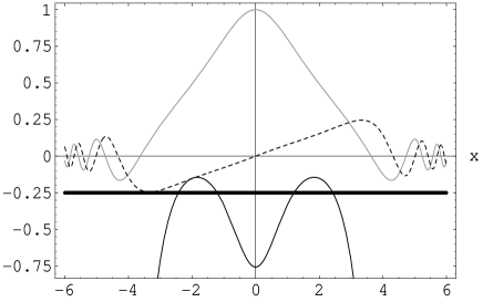
Figure 1: The potential $V(x)$ (black), the even parity wave function (gray), the odd parity wave function (dashed) and the energy (thick black) for the values of the parameters $\nu=1$ and $A_{1}=\frac{1}{144}$. The vertical axis represents both the unnormalised amplitude of the wavefunction and the energy scale in appropriate units.

The example of equation (4) is not an isolated curiosity. In this paper, we deduce various generic properties of degenerate bound states supported by non-singular, but unbounded, potentials and show how to explicitly construct large classes. We then discuss the possibility of realising them experimentally. Note that although the unbounded systems we study generally have non-Hermetian boundary conditions, they do have real bound state solutions.

Now, linear second-order differential equations of the form (1) are very well studied Tit , and we quote here two results for our use. Firstly, if the potential is unbounded below then $k^{2}\to+\infty$ as $x\to\pm\infty$ and so all solutions of (1) will be oscillatory GR . That is, all solutions will have an infinite number of zeros. This is intuitively reasonable as in this case the equation looks asymptotically like that for a classical harmonic oscillator but with increasing frequency.

Secondly, another well-known theorem GR states that the zeros of two independent solutions of (1) interlace: between any two zeros of one solution there will be exactly one zero of the other solution. Again the $\sin$ and $\cos$ solutions of the classical harmonic oscillator equation illustrate this.

Also, as we noted above, for degenerate bound states we need (2) to be nonzero, so at least one of the bound states, say $\psi_{1}$, must have a diverging slope at infinity. Combining this with the fact that the state must be oscillatory means that the zeros must get closer together as $x$ increases. But since the other independent state, $\psi_{2}$, has interlacing zeros with $\psi_{1}$, its zeros too must get closer together and it too must have a slope that diverges at infinity.

We now proceed to construct classes of such degenerate bound states and the potentials that support them. The discussion above suggests we adopt the following ansatz for our pair of degenerate states

$$\phi_{+}(x)=f(x)\cos g(x)$$ (7)

$$\phi_{-}(x)=Bf(x)\sin g(x)$$ (8)

where $B$ is a constant and the functions $f,g$ need to be twice differentiable for use in (1). Integrability of the wavefunctions is achieved by requiring

$$\int dx\ f^{2}<\infty\,.$$ (9)

Substituting (7),(8) into (2) we find a constraint on $g$,

$$g(x)=\int^{x}{\gamma\over f^{2}(x^{\prime})}\ dx^{\prime}\,,$$ (10)

where we have set $\gamma\equiv C/B$. For this integral to be well-defined we require $f$ to be nonzero in the domain $(-\infty,\infty)$. So we choose, $f(x)>0$.

The corresponding potential can be re-constructed using (7,10) in (1),

$$V(x)-E={f^{{}^{\prime\prime}}\over f}-{\gamma^{2}\over f^{4}}\,.$$ (11)

Choosing a reference point such as $V(0)=0$, fixes the energy of the degenerate bound states. We can make the potential symmetric by requiring $f(x)=f(-x)$, and then we see that $\phi_{+}$ is parity even while $\phi_{-}$ is odd, that is, the degenerate states have opposite parities.

In summary, starting with any twice-differentiable, square-integrable and positive function $f(x)$ defined on the real line, we have an associated potential given by (11). The potential is clearly nonsingular and diverges to minus infinity as $x\to\pm\infty$ due to the $\gamma/f^{4}$ term. Note that the rate at which the potential falls off at infinity is directly correlated with how localised the bound states (7,8) are, both being determined by the function $f$. Since $V(x)=V(-x)$ the potential has an extremum at the origin.

Choosing $f(x)={1\over(\cosh x)^{\nu/2}}$ gives the example of Ref.koleykar . There is clearly a very wide choice in constructing other explicit examples, such as $f(x)=\exp(-x^{2})$ which also gives rise to exponentially localised bound states. Before we look at another example from this class let us discuss some features of the solutions in the class (7),(8) that are independent of the specific form of $f$.

Since the energy is finite, so $E\equiv<H>=<T+V>$ must be finite. But from (7,9) and (11) we see that $<V>$ generally diverges, getting large negative contributions at infinity. This means that the average kinetic energy, $<T>$, must likewise be divergent, getting large positive contributions at infinity. This is consistent with the fact that the state has diverging slope at infinity, meaning diverging momentum. Related to the diverging kinetic energy is the fact that the states (7),(8) clearly have an infinite number of nodes, see (10) and (9), whose density increases with $x$.

Let us now look in detail at another example from the above class of solutions,

$$f(x)={a\over\sqrt{1+x^{2}}}$$ (12)

with $a$ a constant. This gives $g(x)={\gamma\over a^{2}}({x^{3}\over 3}+x)$ for use in the corresponding bound states (7,8). The potential is

$$V(x)-E=\frac{2x^{2}-1}{\left(x^{2}+1\right)^{2}}-\frac{\gamma^{2}}{a^{4}}\left(x^{2}+1\right)^{2}\,.$$ (13)

In addition to the extremum at $x=0$ the potential has at most two maxima located at $x=x_{\pm}$, obtained as solutions of the algebraic equation

$$\left(x_{\pm}^{2}+1\right)^{4}-\frac{a^{4}}{\gamma^{2}}\left(2-{x_{\pm}}^{2}\right)=0\,.$$ (14)

It is easy to see from a graphical analysis that real positive solutions, $x_{\pm}^{2}$, to (14) exist, and hence the maxima exist, only if $\gamma^{2}<2a^{4}$ : otherwise the bound states occur above the convex potential! When the well forms, the height of the potential at the barriers is given by

$$V(x_{\pm})-E=\frac{3({x_{\pm}}^{2}-1)}{(x_{\pm}^{2}+1)^{2}}\,.$$ (15)

To see whether the bound states are inside or outside the well, set $z=x_{\pm}^{2}>0$ and rewrite (14) as a condition on $\gamma$,

$$\gamma^{2}={a^{4}(2-z)\over(z^{2}+1)^{4}}\,\,,$$ (16)

the right-hand-side of which is a decreasing function of $z$. Thus we see again that we need $\gamma^{2}<2a^{4}$ for a well to form. Furthermore (15) shows that $z=1$ is a critical value: for $z<1$ the bound states are outside the well and they move inside when $z>1$. Using this in (16) shows that even after the well forms, the bound states remain outside if $\gamma^{2}>a^{4}/16$.

The $\gamma^{2}=0$ limit is interesting as it corresponds to $C=0$ in (2) and hence no degeneracy. What happens is that as $\gamma\to 0$, the oscillations of both states occur further out, and since the parity odd state has the $\sin(\gamma...)$ factor, it goes to zero in any finite domain. Eventually at strictly $\gamma=0$, the parity odd state drops out of the spectrum and the parity even state becomes non-oscillatory, $\phi_{+}\to f(x)$, representing the ground state of the potential (13) with $\gamma=0$. Since the $\gamma=0$ potential goes to a finite constant at infinity, which is conventionally choosen to be zero, so its ground state, $\phi=f$, is a zero energy bound state.

Figure 2: The potential ($V(x)-E$) in Eqn. (13) for $\gamma^{2}=0$.

The $\gamma^{2}=0$ version of (13) is a volcano potential with a finite bottom, Figure 2. Such potentials also occur naturally in braneworld scenarios grem , the normalisable zero energy ground state corresponding to a stable graviton localised near the brane. Generalisations of (12) which lead to potentials with similar properties are discussed elsewhere kp2 .

So far we have illustrated one class of potentials. Noting that $\sin z$ is related to the spherical Bessel function $J_{1/2}(z)$, one may replace the trigonometric functions in (7),(8) by Bessel functions of fractional order $J_{\pm\mu}(z)$ to obtain a different class. The relation (10) remains essentially the same but the resulting expression for the potential is more complicated. We discuss the Bessel function ansatz and others in kp2 .

Given the fact that degenerate bound states have been shown to exist in very large classes of non-singular potentials, depending on a function $f$ with rather mild constraints, we think that it should be possible to observe such states under laboratory conditions. In particular, advances in technology have enabled one to engineer specific mesoscopic structures meso and we feel that these might be ideal for the purpose at hand. The generic features of the states that one is looking for are: One dimensional degenerate bound states of opposite parity supported by non-singular potentials that are unbounded below at infinity.

The oscillatory bound states we have discussed bear some resemblance to von Neumann-Wigner bound states bic that occur in the continuum. While the von Neumann-Wigner states are also oscillatory, they are typically supported in three dimensions by spatially oscillatory potentials ( von Neumann-Wigner bound states have also been studied in low dimensions for specific geometries with particular boundaries, see for example, lowBIC ). The main differences are that in our case the potential is non-oscillatory and there is a pair of degenerate states. Furthermore, in the idealised case we have discussed so far, the degenerate states can occur not only above the potential well but also inside it.

Of course bottomless potentials, like the singular potentials discussed in loudon ; cohen ; pathak are mathematical idealisations and one expects realistic potentials that approximate these to still display the main characteristics. If our bottomless potential is cut off at some large distance then we expect the bound states to be still essentially degenerate, oscillatory and appearing close to the top of the potential. Given that von Neumann-Wigner states have been detected experimentally cap , we think that the degenerate states we have discussed in this paper may also be observable.

We note that volcano potentials with a finite bottom have been studied before semi , but we are unaware of any investigations which focus on possible degenerate bound states at the top of such potentials that have a large height compared to the depth of the well.

There are many interesting questions regarding potentials of the form (11). For example, do they support bound states other than the ones used to construct them? Also, as noted above, in the $C\to 0$ limit the expression (11) becomes a bounded potential expressed in terms of a function $f$ that may be interpreted as the ground state of the system (since it is nodeless)–this suggests some connections with supersymmetric quantum mechanics susy . We hope to return to these and other questions at a later stage kp2 .

References

- (1) L. D. Landau and E. M. Lifshitz, Quantum Mechanics (Pergamon Press, Oxford, 1977), Pg. 60
- (2) R. Loudon, Am. J. Phys. 27, 649 (1959).
- (3) J. M. Cohen and B. Kuharetz, J. Math. Phys. 34, 12 (1993).
- (4) K. Bhattacharyya and R. K. Pathak, Int. J. Quantum Chem. 59, 219 (1996); J-M. Levy Leblond and F. Balibar, Quantics: rudiments of quantum physics (North Holland, 1990), Pg. 357.
- (5) K.K. Wan, From Micro to Macro Quantum Systems, Chap. 6, (Imperial College Press, 2006).
- (6) A. Messiah, Quantum Mechanics, Pgs 98-106, (Dover Publications, 1999).
- (7) J. von Neumann and E. Wigner, Phys. Z 30, 465 (1929); F. H. Stillinger and D. R. Herrick, Phys. Rev. A 11, 446 (1975).
- (8) C. Bender, Introduction to PT symmetric quantum theory, quant-ph/0501052.
- (9) A. Mostafazadeh, J. Math. Phys. 43, 205 (2002); J. Phys. A 36, 7081 (2003).
- (10) V. Buslaev and V. Grecchi, J. Phys. A 26, 5541 (1993); H.F. Jones and J. Mateo, Phys. Rev D 73, 085002 (2006).
- (11) L. Randall and R. Sundrum, Phys. Rev. Lett. 83, 4690 (1999); C. Csaki, J. Erlich, T. J. Hollowood, and Y. Shirman, Nucl. Phys. B 581, 309 (2000); R. Koley and S. Kar, Class. Quant. Grav. 22, 753 (2005); N. Barbosa-Cendejas and A. Herrera-Aguilar, Phys. Rev D 73, 084022 (2006).
- (12) R. Koley and S. Kar, Phys.Lett. A 363, 369 (2007)
- (13) H-T. Cho and C-L. Ho, quant-ph/0606144
- (14) E Caliceti, V. Grecchi and M. Maioli, Commun. Math. Phys. 157,347 (1993); J. Zamastil, J. Cizek and L. Skala, Phys. Rev. Letts. 84, 5683 (2000); J. Zamastil, V. Spirko, J. Cizek, L. Skala and O. Bludsky, Phys. Rev. A 64, 042101 (2001); F. J. Gomez and L. Sesma, Phys. Letts. A 301, 184 (2002).
- (15) E.C. Titchmarsh, Eigenfunction expansions associated with second-order differential equations, Part I (2nd Edition, Oxford University Press, 1962), Pgs 92-94 and Pgs 123-125.
- (16) I.S. Gradshteyn and I.M. Ryzhik, Tables of Integrals, Series and Products, (Academic Press, 1980).
- (17) M. Gremm, Phys. Lett. B 478, 434 (2000).
- (18) S. Kar and R. Parwani, in progress.
- (19) F. Capasso, J. Faist, and C. Sirtori, J. Math. Phys. 37 4775 (1996); D.F. Holcomb, Am. J. Phys. 67, 278 (1999).
- (20) P.S. Deo and A.M. Jayannavar, Phys. Rev. B 50, 11629 (1994); S. Longhi, quanth-ph/0612152, and references therein.
- (21) F. Capasso, C. Sirtori, J. Faist, D. L. Sivco, S. N. G. Chu and A. Y. Cho, Nature 358, 565 (1992).
- (22) L. L. Chang, L. Esaki, R. Tsu, Appl. Phys. Lett. 24, 593 (1974); Z. I. Alferov, Rev. Mod. Phys. 73, 767 (2001); T.C. Au Yeung, Yabin Yu, W.Z. Shangguan and W.K. Chow, Phys. Rev. B 68, 075316 (2003).; M. M. Nieto, Phys. Lett. B486,414 (2000).
- (23) F. Cooper, A. Khare and U. Sukhatme, Phys.Rept. 251 267 (1995).