N₂H⁺ and N₂D⁺ in Interstellar Molecular Clouds. II – Observations

Abstract

We present observations of the $J$=1–0, 2–1, and 3–2 rotational transitions of N₂H⁺ and N₂D⁺ towards a sample of prototypical dark clouds. The data have been interpreted using non–local radiative transfer models. For all sources previously studied through millimeter continuum observations, we find a good agreement between the volume density estimated from our N₂H⁺ data and that estimated from the dust emission. This confirms that N₂H⁺ depletion is not very efficient in dark clouds for densities as large as 10⁶ cm^-3, and also points out that a simultaneous analysis based on mm continuum, N₂H⁺ and N₂D⁺ observations should lead to reliable estimates for the temperature and density structure of cold dark clouds.

From multi–line modeling of N₂H⁺ and N₂D⁺, we derive the deuterium enrichment in the observed clouds. Our estimates are similar or higher than previous ones. The differences can be explained by the assumptions made on the cloud density profile, and by the chemical fractionation occurring in the clouds. For two of the observed objects, L183 and TMC2, multi–position observations have allowed us to derive the variation of the N₂D⁺/N₂H⁺ abundance ratio with the radius. We have found that it decreases by an order of magnitude for radii greater than a few 0.01 pc (i.e. outside the central cores). Inside the dense condensations, the fractionation is efficient and, compared to the abundance ratio expected from statistical considerations based on the cosmic D/H ratio, the deuterium enrichment is estimated to be $\simeq$ 0.1–0.5 10⁵.

An important result from our observations and models is that the interpretation of deuterated molecular species emerging intensities in cold dark clouds requires specific radiative transfer modeling because the excitation conditions for the deuterated species can be quite different from those of the main isotopologue. Moreover, the use of three rotational lines for N₂H⁺ and N₂D⁺ allows to constrain the size of the emitting regions for each species and to determine accurately the volume density. This enables to draw a detailed picture of the spatial variation of deuterium enrichment.

1. Introduction

Over the past decades, important efforts have been devoted to improve our understanding of the physical conditions in protostellar clouds. These studies have enabled to draw an evolutionary sequence of the stages prior to the formation of protostars, through the morphological, dynamical and chemical characteristics of the clouds. Recent progress in detection capabilities in the far infrared, sub–mm and mm windows, have permitted to constrain the density distribution of molecular clouds through measurements of dust absorption and emission (see e.g. Ward–Thompson et al., 1994, 1999). It has been found that the geometrical structure of cold dark clouds is consistent with an inner region of nearly constant density and a surrounding envelope that has a density which decreases as a power law. The density distribution thus obtained is often used as a starting point for molecular line studies and allows to constrain the spatial distribution of the molecules (see e.g. Tafalla et al., 2004). Moreover, from NH₃ inversion lines it has been found that the clouds are nearly isothermal (Benson & Myers, 1989; Tafalla et al., 2004). Such observational constraints are of great interest to understand the physical mechanisms that drive the collapse. However, the balance between gravitational energy and support mechanisms such as thermal pressure, turbulence or magnetism is yet to be understood (Aikawa et al., 2005). Moreover, theoretical studies predict that the initial conditions strongly affect the way the collapse of the cloud evolves. In particular, time dependent studies, which couple both dynamical and chemical processes, have shown that molecules can be used as tools to probe the stage of evolution prior to the formation of protostars. These studies also predict that deuterium fractionation increases with time and that the D/H ratio can reach high values for a variety of species (Roberts et al., 2003).

The goal of this work is to put observational constraints on the spatial structure of a sample of dark clouds through observations of a late type molecule, N₂H⁺, and of its deuterated isotopologue N₂D⁺. These molecules are well adapted to probe the innermost dense regions of dark clouds due to their high dipole moments and also because they are weakly depleted onto dust grains. While molecular observations are a very powerful tool to derive the physical and chemical conditions of the gas in these regions, the interpretation of the observations needs essential informations on molecular physics data, such as collisional rate coefficients, line intensities and frequencies. Molecules often used as tools, like N₂H⁺, have been interpreted so far with crude estimates of these parameters. Recently, Daniel et al. (2005) have computed collisional rate coefficients between N₂H⁺ and He for the range of temperatures prevailing in cold dark clouds and low mass star forming regions. Daniel et al. (2006) (hereafter referred to as Paper I) have modeled, using these new rates, the emission of N₂H⁺ in dark clouds. A wide range of physical conditions has been explored in order to have a general view of the different processes that could lead to the observed intensities of N₂H⁺ hyperfine lines.

Observations are described in section 2. In section 3 we present the results obtained for each cloud and we derive the physical conditions of the gas as well as N₂H⁺ and N₂D⁺ abundances. The conclusions are given in section 5. The excitation processes occurring for deuterated species are analyzed in the Appendix.

2. Observations

N₂H⁺ and N₂D⁺ observations were performed during several observing sessions. Additionally, we make use of N₂D⁺ data already discussed by Tiné et al. (2000).

Observations of the N₂D⁺ $J$=2–1 line have been obtained at the IRAM–30m telescope (Granada, Spain) in July 2000 during average weather conditions. The pointing was checked regularly on nearby continuum sources, and the focus was checked on small planets. The data have been taken in frequency switching mode, with the mixers connected to the versatile, high spectral resolution, correlator VESPA. The N₂D⁺ $J$=1–0 data have been taken in August 2004 when the tuning range of the 3mm mixers was extended to frequencies lower than 80 GHz. Simultaneous observations of N₂D⁺ $J$=3–2 were performed using two mixers tuned at this frequency. The system temperature was $\sim 250$ K at 77 GHz and $\sim 500$ K at 231 GHz. Particular care was given to the intensity calibration as the mixer tuning is done without side band rejection at these low frequencies. The image side band gain has been measured on an offset position or a continuum source for each object, and applied during the data processing.

Further observations of the $J$=1–0, 2–1 and 3–2 lines of N₂H⁺ and of the N₂D⁺ $J$=3–2 line were carried out in January 2005 with the IRAM–30m telescope. Four receivers tuned at the frequency of these lines were used simultaneously. Pointing was checked every hour on continuum sources close to the targets. The relative alignment of the receivers was checked with Saturn and Jupiter and found to be better than 2.0”. Our observations indicate that the offsets on the sky from the pointing derived with the 3 mm receiver were 1.0”, 2.0” and 1.0” for the 2 mm, 1 mm low frequency and 1 mm high frequency receivers respectively. Focus was checked at the beginning and end of each observing shift. It was found to be stable for the entire observing run.

The weather was excellent during observations with a typical water vapor amount above the telescope site of $\simeq$ 1.0 mm, or even better. Calibration was performed using two absorbers at ambient and liquid nitrogen temperatures. The ATM package (Cernicharo, 1985; Pardo et al., 2001) was used to estimate the significant atmospheric parameters for the observations. The typical system temperatures were 100 K, 1000 K and 250 K at 3, 2 and 1 mm respectively. The $J$=2–1 line was observed in upper side band which avoided the possibility of rejecting the image side band in the 30–m receivers. The large system temperature for this transition is due to the high opacity of the atmosphere at 186 GHz and to the fact that the frequency is at the edge of the tuning range of the receiver. Calibration uncertainties for the $J$=1–0 and 3–2 lines are well below 10% (the standard calibration accuracy under good weather conditions). However, the $J$=2–1 line has a larger uncertainty due the effects commented above, and, in order to have an estimate of the calibration accuracy we observed the continuum emission of Jupiter, Saturn and Mars at different elevations. We have found that the intensity of the $J$=2–1 transition was always compatible with the expected one. However, these double side band observations of the planets are not very sensitive to the side band rejection. Nevertheless, these data allow us to derive beam efficiencies for each frequency. They are in excellent agreement with those published for the 30–m IRAM telescope. For some strong sources we observed several times a reference position and we noted that the $J$=2–1 line intensity had calibration errors up to 20% depending on the elevation of the source. We conclude that with the configuration adopted for the 2 mm receiver, the upper signal side band has a gain of 0.35 rather than 0.5 (perfect DSB). This fact introduces systematic errors in the determination of the sky opacities. It is impossible to estimate the actual error for each source. Hence, for the $J$=2–1 line we assume a typical calibration error of 20%. Nevertheless, most observed $J$=2–1 intensities agree with those expected from the results of the $J$=1–0 and 3–2 lines (see Sect. 3). Only for TMC2, L1489 and L1251C it has been necessary to correct the $J$=2–1 intensities by multiplicative factors of, respectively, 0.8, 0.8 and 0.85 in order to have data consistent with the well calibrated $J$=1–0 and 3–2 lines.

The observations were performed in frequency switching mode. As all sources have narrow lines, the baseline resulting from folding the data has been removed by fitting a polynomial of degree 2. Figure 1 shows the N₂H⁺ and N₂D⁺ observed lines in selected sources and Table 1 gives the position of the clouds observed in this paper (see section 3). The intensity scale is antenna temperature, T${}_{A}^{*}$. In order to compare the results of our models with observations, we have to convolve model results with the beam pattern of the 30–m IRAM telescope. We have adopted half power beam widths (HPBW) of 27”, 13.5” and 9”, beam efficiencies of 0.76, 0.59 and 0.42, and error beams of 350”, 220”, and 160” for the $J$=1–0, 2–1 and 3–2 lines of N₂H⁺. For N₂D⁺, we adopted HPBW’s of 32”, 17” and 10.5”, beam efficiencies of 0.79, 0.69 and 0.52 and the same error beams as for N₂H⁺ lines. The whole data set for all observed sources is shown in Figures 3 to 15.

3. Results

Over the past decades, mm continuum observations and star count analysis (Ward–Thompson et al., 1994) have revealed that the density structure of cold dense cores closely matches a Bonnor–Ebert sphere, with an inner region of nearly uniform density and steep outer edges where the density decreases as r^-p with p = 2 – 2.5. This description is valid for r $<$ 0.1 pc typically, and at larger scales (0.1 – 1 pc), the density structure of the outer envelope has been shown to vary from sources to sources. For example, Cernicharo et al. (1985) have found that a shallow density profile, n(r) $\propto$ r^-1/3, is adequate to model the density structure of the envelope of the Taurus–Auriga complex. In this section, we use a density profile which corresponds to n(r) = n₀ for r $<$ r₀ and n(r) = n₀(r₀/r)² for r $>$ r₀. In order to characterize the clouds, we determine the value of the central density, i.e. n₀, and the radius of the inner flat region, i.e. r₀. For L1517B, we compare the results obtained using this density profile with the phenomenological density law used in Tafalla et al. (2004).

The observed line profiles for N₂H⁺ and N₂D⁺ $J$=1–0, 2–1, and 3–2 lines are shown in Figures 3 to 15. In order to model our data we have found that some additional constraints were necessary. In particular the extent of the emission has been found to be a critical parameter to derive physical conditions. Our data are in most cases related to one single observed position (except for L183 for which we have a map in several transitions). Fortunately, some clouds presented in this section have been mapped in the $J$=1–0 transitions of N₂H⁺ by Caselli et al. (2002), Tafalla et al. (2004), and Crapsi et al. (2005) (In the discussion of the sources, if not specified, N₂H⁺ maps refer to data from Caselli et al. (2002)). For six sources (L63, L43, L1489, L1498, L1517B, and TMC–2) they have reported $J$=1–0 integrated intensity versus impact parameter. Thus, we have checked that the profile of the $J$=1–0 integrated intensity provided by our models was consistent with those data. For the other clouds, similar data could not be found in the literature.

The radiative transfer models aim at reproducing our $J$=1–0, 2–1 and 3–2 line intensities and the $J$=1–0 radial emission profile. A discussion concerning the assumptions made to model N₂D⁺ is given in the Appendix (that deals in particular with the determination of collisional rate coefficients for the isotopologue of N₂H⁺). Observed positions, central line intensities and adopted distances to the sources are given in Table 1. We report in the same table the $J$=1–0 emission half power radius (noted $r$). This corresponds to the radius which encloses half of the $J$=1–0 total intensity which emerges of the cloud. The convolution of the emerging line intensities with the telescope beam pattern has been done taking into account the characteristics of 30–m IRAM radio telescope (see section 2) and those of the 14–m FCRAO antenna. For the latter we have used a HPBW of 54” at 91 GHz and a beam efficiency of 0.51. Nevertheless, the error beam size for the FCRAO antenna is not known but must be taken into account. In our modeling, we arbitrarily assume a size of 180”. As quoted above, the radial intensity profile enables to constrain the way density and abundance vary through the cloud. We stress that the density profiles determined in the following section depend essentially on the observations of the $J$=1–0 line. Hence, an accurate description of the radiation pattern of the FCRAO antenna is needed to obtain the best estimates for the physical parameters of the clouds. We have checked the effect of introducing different error beam sizes for the FCRAO antenna, and the largest differences are obtained when the error beam is not taken into account, which leads to $J$=1–0 line intensities 20–30% lower for the same physical conditions and source structure. This effect could be compensated by increasing the size of the central core, r₀, by 5”–10”, decreasing its density, n₀, and increasing the abundance of N₂H⁺ in the outer region of the clouds.

For some sources, we have included infall velocity fields in order to reproduce the spectral features seen in the $J$=2–1 line. The profiles used consist of a $v\propto r$ function which corresponds to infalling cores for all sources, except for L1517B. Despite the inclusion of these velocity fields, we have observed frequency offsets between the observations and the models. In table 4, we report the V_LSR determined from our $J$=1–0 data, the corrections to this value for the other lines (V_LSR and corrections are determined by a $\chi$ square fitting), and the velocity gradient found in the sources. For all of them, we find that the $J$=2–1 and $J$=3–2 lines have V_LSR $\sim$ 30 m s^-1 larger than the V_LSR of the $J$=1–0 line. This would be consistent with the view of a static core with an infalling envelope as the $J$=2–1 and $J$=3–2 lines arise from the densest part of the cloud. However, we think that the effect, 20 and 30 kHz for the $J$=2–1 and $J$=3–2 lines respectively, is within the accuracy of the laboratory frequencies of N₂H⁺ (see e.g. Amano et al., 2005). Consequently, the range of model parameters is limited by the laboratory accuracy in the frequencies.

3.1. Individual core properties

In this section, the cloud physical parameters (see Tables 2 and 3), obtained from the modeling of our data, are discussed. In the following discussion, we use the notation $r_{D}$ $\equiv$ X(N₂D⁺)/X(N₂H⁺) to refer to the isotopologues abundance ratio. This quantity differs from the column density ratio (referred to as $R$ $\equiv$ N(N₂D⁺)/N(N₂H⁺)) in the case of three clouds (L63, TMC2 and the two molecular peaks in L183) for which $r_{D}$ has been found to change with radius. R represents in all cases an averaged value along the line of sight of the N₂H⁺ volume density.

For each cloud, the error bars quoted for the physical parameters are derived by use of a reduced $\chi^{2}$. These are obtained by assuming that the parameters of the models are independent and thus, it does not account for the correlation among them. Nevertheless, it gives an indication on the sensitivity of the emerging spectra to the model’s parameters. The same criterion was used for both N₂H⁺ and N₂D⁺ spectra. The uncertainty on $r_{D}$ is then found important due to the lower signal to noise ratio of the N₂D⁺ data and this leads to large error bars for the N₂D⁺ column density (varying from 20% to 100% depending on the source) while typically, the N₂H⁺ column density is estimated with an accuracy of 10-20 %.

3.1.1 L1517B

Modeled lines and observations of the $J$=1–0 and $J$=2–1 transitions of N₂H⁺ and N₂D⁺ are shown on figure 3. When comparing the line profiles of the two isotopologues, it is important to note the differences which are introduced by their respective abundances, i.e. opacities (see Paper I, ). We see that the intensity ratio between the different $J$=1–0 hyperfine components are best reproduced for N₂D⁺ which is optically thinner than N₂H⁺. This fact supports the idea that hyperfine intensity anomalies are due to radiative effects which occur at high opacities. For the $J$=2–1 lines of the two isotopologues, we see that the main central emission component is self absorbed for N₂H⁺ while it is not for N₂D⁺. Moreover, as commented in Paper I, the line profile seen in the $J$=2–1 line of N₂H⁺ is characteristic of expanding flows.

A detailed study of L1517B has been reported in Tafalla et al. (2004) where the structure of the cloud is derived from maps of the NH₃ inversion line and 1.2 mm continuum emission. The position we observed corresponds to the N₂H⁺ peak intensity given by Caselli et al. (2002), which is situated at (+15”,+15”) of the N₂H⁺ emission peak in the higher resolution map reported by Tafalla et al. (2004). The latter position is also a maximum of the 1.2 mm emission map. In our models we took into account the $J$=1–0 and $J$=3–2 lines reported by Tafalla et al. (2004) towards the continuum peak. On figure 2, we compare the $J$=1–0 radial integrated intensity of our model to the observational data reported in the latter study.

To characterize the velocity structure of L1517B, we introduced a linear outward gradient of 1.4 km s^-1 pc^-1 for radii beyond 20”. As pointed out in Paper I, it is rather difficult to constrain velocity fields from observations of the $J$=1–0 and $J$=3–2 lines of N₂H⁺, while the larger opacity of the $J$=2–1 line enables a better estimate. From observations of CS emission lines, Tafalla et al. (2004) derived a value for the outward gradient of 2 km s^-1 pc^-1, for radii larger than $\sim$ 70”. Hence, this velocity field is consistent with their observations of the $J$=1–0 and $J$=3–2 lines of N₂H⁺ observed towards the central position.

On Figure 2, we compare the $J$=1–0 radial intensities obtained with two types of density profiles. The first is the one quoted above (labeled (1) in Table 2) and the second corresponds to the phenomenological profile used by Tafalla et al. (2004) (labeled as (2)). Using the profile (2), we obtain the same estimate than in the latter study, i.e. n₀ = 2.0 10⁵ cm ^-3 and r₀ = 35”. Moreover, we see that with the present observational data, we are rather insensitive to the exact form of the function which describes the density variations in the cloud, since the two density profiles give similar results for both line shapes and the $J$=1–0 integrated intensity profile.

Using the two density profiles mentioned above, we also derive different estimates for the N₂H⁺ abundance, i.e. 1.6 10^-10 with (1) and 2.5 10^-10 with (2). In the latter case, our estimate is higher by $\sim$ 70% with respect to the one obtained by Tafalla et al. (2004), i.e. X(N₂H⁺) = 1.5 10^-10. The difference is due to the use of different sets of collisional rate coefficients in each studies.

We have determined the D/H ratio that allows to reproduce the $J$=2–1 line of N₂D⁺ for the two density profiles. For the density profile (1), we derive R = 0.12${}^{+0.04}_{-0.03}$ which is a factor 2 higher than the estimate of 0.06 $\pm$ 0.01 obtained by Crapsi et al. (2005) toward the density peak position.

Benson & Myers (1989) have estimated a mass of 0.33 M_☉ within a radius of 1.4’, which corresponds to a mean volume density of n(H₂)=6 10³ cm^-3. For the same radius, we obtain a mass of 2.5 M_☉. On the other hand, the analysis of emission maps at 850 $\mu$m and 450 $\mu$m (Kirk et al., 2005) lead to an estimate of n(H₂) $\sim$ 4–5 10⁵ cm^-3, in qualitative agreement with the central density assessed from our N₂H⁺ data.

3.1.2 L183

L183 is a well studied object due to its proximity (d=110 pc). It has a non spherical shape with a north–south axis in the density distribution. Recent studies point out a complex chemistry in the cloud, with four main molecular peaks showing characteristics which are interpreted as signs of different stages of evolution (Dickens et al., 2000). The N₂H⁺ maximum of intensity is situated near the densest part of the cloud (molecular peak C). A secondary maximum situated $\sim$ 3’ to the north (molecular peak N) is also seen in the N₂H⁺ intensity map. For this source, the observed position for molecular peak C corresponds to the intensity peak as given by Caselli et al. (2002). It is placed at (-5”,+15”) with respect to the peak position of the higher resolution maps given by Dickens et al. (2000) and Pagani et al. (2005).

Figure 4 shows peak C observations and models of the $J$=1–0, 2–1 and 3–2 transitions of N₂H⁺, and of the $J$=3–2 transition of N₂D⁺. Figure 5 shows the $J$=1–0 and 3–2 lines of N₂H⁺ and the $J$=1–0, 2–1 and 3–2 lines of N₂D⁺ for peak N. Figures 6 and 7 present maps of the $J$=1–0 and 2–1 lines of N₂D⁺ obtained towards peak C, the latter being obtained with the same data as in Tiné et al. (2000).

There are a number of studies regarding the dust emission properties of L183 (e.g. Kirk et al. (2005) at 450 and 850 $\mu$m, Juvela et al. (2002), Pagani et al. (2003) at 200 $\mu$m and Pagani et al. (2005) at 1.2 mm). From these studies, it seems that the region of molecular peak C is associated with two continuum sources FIR1 (south) and FIR2 (north) separated by $\sim$ 1.5’. The region of FIR1 and FIR2 corresponds to the maximum extinction and minimum temperature in the cloud (Juvela et al., 2002). Also, there might be a gradient of temperature in this region or changes in the composition of the grains since FIR1 is detected at 200 and 450 $\mu$m but remains undetected at 850 $\mu$m. Moreover, the emission peak FIR2 at 850 $\mu$m is shifted to the North compared to that at 200 and 450 $\mu$m (Kirk et al., 2005), while the 1.2 mm peak position is shifted to the South. It is worth noting that the maxima of the 1.2 mm and N₂H⁺ maps reported in Pagani et al. (2005) do not coincide. From this study, it appears that the maxima of these two maps are shifted by $\sim$ 25” and that the H₂ volume density reaches 2 10⁶ cm^-3 at the position of the 1.2 mm map emission peak. For simplicity, we have modeled the observations of peak C assuming that the density center of our model is at the position of the N₂H⁺ emission peak (i.e. offset by (+5",-15") with respect to the coordinates given in table 1).

For the spectra belonging to peak N, our observations are off by (+2”,-40”) with respect to the reference position given by Dickens et al. (2000). We have assumed in our models that the density peak is centered at the position of our observations which corresponds to the secondary maximum in the N₂H⁺ map.

For peak C, in order to fit the observed asymmetry in the $J$=2–1 transition, we have included a velocity gradient of $\Delta$v = -0.2 km s^-1 pc^-1. As discussed in Paper I, this line is sensitive to small velocity gradients, due to the presence of multiple hyperfine components in a small frequency interval. For peak N, no velocity gradient was included since, for this position, the observed lines are insensitive to such small velocity fields (the $J$=2–1 line was not observed). It is worth noting that the $J$=2–1 transition of N₂H⁺ obtained towards peak C has a peculiar shape that is not observed in any other cloud of the present sample. Hence, the abundance profile obtained for this source is unique, among all our models, since we find that the best agreement between models and observations is obtained by increasing the abundance at large radii.

For the two peaks, we obtain similar N₂H⁺ abundances, but different density profiles: peak C is more dense and centrally peaked than peak N. For the former position, our density estimate is consistent with that obtained from sub–mm observations, i.e. n(H₂) = 10⁶ cm^-3 (Kirk et al., 2005).

In order to model the N₂D⁺ map shown in Figures 6 and 7, the relative abundance has been set to $r_{D}$ = 0.43 for radii below r $\sim$ 0.021 pc. For larger radii, the relative abundance is lowered to 0.05. Note that this decrease in abundance is necessary to reproduce the line shapes as it reduces the self–absorption induced by the external layers of the cloud, in the $J$=2–1 main component of N₂D⁺. On the contrary, the main component of the $J$=2–1 transition of N₂H⁺ is strongly self–absorbed and is better reproduced by increasing the N₂H⁺ abundance at the outermost radii. Since our model considers spherical geometry while the morphology of the cloud is extended along a North–South axis, we have failed to reproduce the $J$=2–1 transition for the whole map. Hence, the intensities are well reproduced for declinations between $\delta$ = -20” and +20” but are underestimated along the North–South axis. Toward the position given in table 1, we find a column density ratio R = 0.33${}^{+0.16}_{-0.11}$ which is similar to the one obtained by Tiné et al. (2000) at a position offset by $\sim$ 5" to the north, i.e. R = 0.35. This value is higher than the one obtained by Crapsi et al. (2005) at a position offset by (-5",-15"), i.e. R = 0.22 $\pm 0.04$.

From the observations towards peak N, we obtain values for the deuterium enrichment of $r_{D}$ = 0.76 for radii below 5 10^-3 pc and 0.05 beyond. Note that the radius which encloses the central D–rich region is determined from a single position analysis. Because the angular size of this central region is intermediate between the HPBW of the $J$=1–0 and 3–2 lines of N₂D⁺, (32” and 10” respectively), the $J$=3–2 line is favored compared to the $J$=1–0 one. In order to better constrain the variation of the D/H ratio with radius, observations at different positions are needed. For peak N, we derive a column density ratio of R = 0.15 .

Recently, a similar work based on N₂H⁺ and N₂D⁺ observations was carried out by Pagani et al. (2007) for molecular peak C. This latter study differs from ours in the location of the center of the density profile: it was set coincident with the maximum of the 1.2 mm map which is shifted $\sim$ 25" to the south compared to that assumed in the present work. Moreover, the 1D radiative transfer code used in Pagani et al. (2007) work treats line overlap and the convolution with the telescope beam was made using an approximation that takes into account the north-south extent of the cloud. At the position of the 1.2 mm map peak, they found that the temperature ranges from 7K (from N₂H⁺ data) to 8K (from N₂D⁺ data) and that the maximum H₂ density is 3 times higher than that derived in the present work. Note that the density profile derived here and the "best model" profile in Pagani et al. (2007) are similar beyond 30": the latter corresponds to densities which are higher by $\sim$ 25%. The main difference concerns the N₂H⁺ abundance profile. Pagani et al. (2007) have found that X(N₂H⁺) drops by a factor $6^{+13}_{-3}$ in the inner 20" region. This decrease is interpreted as depletion and it becomes efficient at densites n(H₂) = 5–7 10⁵ cm^-3. At our position, we do not see evidence for such a strong decrease in abundance: the abundance we find is $\sim$ 1.6 time lower below 40" where the density reach n(H₂) = 2 10⁵ cm^-3. Given that the source strongly departs from spherical geometry, this variation could be a consequence of a mis–interpretation of the real excitation conditions and prevents us to interpret this result as a sign of depletion. Considering the deuterium enrichment, Pagani et al. (2007) find that at the 1.2 mm map peak, $r_{D}$ varies from 0.7 $\pm 0.12$ (inner 6") to 0.05 (beyond 40"), which is consistent with the present findings.

3.1.3 TMC2

In the present study, we report N₂H⁺ and N₂D⁺ observations for two positions towards TMC2 which are separated by $\sim$ 40”. Figure 8 shows the $J$=1–0, 2–1 and 3–2 observed lines of N₂H⁺, and the $J$=3–2 line of N₂D⁺ for the central position. For the (-33”,-23”) position, N₂H⁺ $J$=1–0 and N₂D⁺ $J$=2–1 lines are shown. Figure 2 shows the $J$=1–0 radial integrated intensity of the model compared to observational data from Caselli et al. (2002).

This source has been mapped in many molecular lines (e.g. C¹⁸O, DCO⁺ and H¹³CO⁺ by Butner et al. (1995), H¹³CO⁺ by Onishi et al. (2002) and C¹⁸O by Onishi et al. (1996)) as well as in 1.2 mm continuum emission by Crapsi et al. (2005). Large scale visual extinction maps covering the whole region are reported by Cernicharo et al. (1984, 1985). Contrary to other clouds, N₂H⁺ and 1.2 mm maps seem to be uncorrelated: while the N₂H⁺ peak has a bright 1.2 mm emission counterpart, there are several maxima in the 1.2 mm map which do not correspond to any N₂H⁺ peak. In this work, we derive an average central volume density of n(H₂) $\sim$ 3.5 10⁵ cm^-3, which is in good agreement with the value of 3 10⁵ cm^-3 derived from the analysis of the 1.2 mm emission. However, this value is higher than the estimates obtained from other molecular species. The discrepancy partly arises from a different spatial location of the molecules (see the map of C¹⁸O reported by Crapsi et al. (2005) and the map of H¹³CO⁺ of Onishi et al. (2002)). On the other hand, N₂H⁺ and NH₃ lines (Myers et al., 1979) seem to arise from the same region and an average volume density of 2.5 10⁴ cm^-3 was derived from the latter molecule. Similar values for the average density are given in Butner et al. (1995), based on C¹⁸O and DCO⁺ lines. Nevertheless, higher density estimates have been obtained using H¹³CO⁺ (Onishi et al., 2002). The map of this molecule shows that two emission maxima are located within the NH₃ map corresponding to regions of average volume density $\sim$ 10⁵ cm^-3.

From NH₃ lines, the mass enclosed within a radius of 3.6’ has been estimated to be $\sim$ 16 M_☉, and from C¹⁸O lines (Onishi et al., 2002), the mass enclosed within 7.8’ is estimated to be $\sim$ 50 M_☉. The density profile given in table 2 corresponds to enclosed masses of 50 M_☉ and 121 M_☉ for the same radii. We stress that the value adopted for r₀ is the most important parameter to derive the mass of the cloud and, in order to obtain similar values than those quoted above and using the same central density, we would have to adopt a value of r₀ $\sim$ 35”. Adopting such a small value for r₀ does not allow to reproduce the $J$=1–0 radial integrated intensity.

To reproduce the N₂D⁺ spectra obtained towards the two positions, we have decreased the abundance ratio by a factor 7 at radii $>$ 0.024 pc. It is worth noting that a single position analysis enables to reproduce independently each one of the two N₂D⁺ spectra, assuming a constant value for $r_{D}$. For the central position, such an analysis leads to a ratio of $r_{D}$ $\sim$ 0.25.

3.1.4 TMC1(NH₃)

Figure 9 shows observations of N₂H⁺ and N₂D⁺ towards two positions separated by $\sim$ 35”. The reference position is given in table 1 and the second position is located at (-35”,+9”). Towards both positions, two velocity components are identified in the observations of the $J$=1–0 line of N₂H⁺. In order to model the faintest component, we have simply added the contribution of two emitting regions. This way of computing the emerging spectra is motivated by the fact that the difference in the V_LSR of the two components is larger than the linewidth: the determined V_LSR are 5.98 km $s^{-1}$ and 5.68 km $s^{-1}$, the former being the most intense one. For both positions, the faintest velocity components have been determined to be similar.

The TMC1 ridge is known to have a complex velocity structure with a velocity gradient of $\sim$ 0.2 km s^-1, perpendicular to the major axis of the ridge (Olano et al., 1988) , and cores at different V_LSR for the same line of sight. Particularly, two components at $\sim$ 5.6 km $s^{-1}$ and 6.0 km $s^{-1}$ have been identified around the cyanopolyyne peak (Tölle et al., 1981). Also, around the ammonia peak, two possible components at V_LSR $\sim$ 5.9 km $s^{-1}$ and 5.3–5.4 km $s^{-1}$ are reported by Hirahara et al. (1992) from observations of C³⁴S transitions, the latter being identified as a low density core. The two V_LSR components identified in this work are also seen in SO observations (Lique et al., 2006).

As for the previous sources, we obtain a higher density estimate than in previous studies based on the emission from other molecules. See for example the detailed analysis of the density structure along the TMC1 ridge reported by Pratap et al. (1997). At the position of the N₂H⁺ peak (ammonia reference position), the density is estimated to be $\sim$ 10⁵ cm^-3 from the analysis of several HC₃N lines. Note that the structure of the cyanopolyyne peak has been probed through interferometric observations (Langer et al., 1995). It has been found that the core of the cloud consists of several high density condensations (n(H₂) $\sim$ 3 10⁵ cm^-3) with diameters ranging from 10” to 30”, which are embedded in a lower density medium. This result was further confirmed by Tóth et al. (2004) who analyzed ISOPHOT images.

From the $J$=2–1 line of N₂D⁺, we derive R $\sim$ 0.10${}^{+0.09}_{-0.04}$ for the ammonia reference position, which is in good agreement with the value of 0.08 reported by Tiné et al. (2000).

3.1.5 L1498

Figure 10 shows the $J$=1–0 line of N₂H⁺, and the $J$=1–0 and 2–1 lines of N₂D⁺. L1498 is a nearby molecular cloud located in the Taurus complex. This cloud has been observed in H₂CO (Young et al., 2004), CS (Tafalla et al., 2004) and N₂H⁺ (Tafalla et al., 2004; Shirley et al., 2005) and its physical properties have been derived from ISOPHOT observations (Langer et al., 2001) and millimeter observations (Shirley et al., 2005).

As for L1517B, a detailed study of L1498 has been done by Tafalla et al. (2004), and we have used this work as a starting point for our models. The position we observed in this source is at (+10”,0”) of the 1.2 mm emission peak. In our model, we have assumed that the center of the density profile corresponds to the continuum peak. Figure 2 shows the $J$=1–0 radial integrated intensity compared to the observational data reported by Tafalla et al. (2004). As noted in that study, a decrease of the abundance in the outer envelope is needed to reproduce the $J$=1–0 radial intensity profile. Otherwise, the intensity would be overestimated at large radii.

The values we have derived for the density and for the N₂H⁺ abundance are consistent with those found by Tafalla et al. (2004). As for L1517B, we derive a higher abundance than in the latter study (X(N₂H⁺)= 2.5 10^-10 compared to 1.7 10^-10). This is related to the use of different collisional rate coefficients and density profiles in each study. Moreover, we derive the same central density, but with a smaller value for r₀ due to the different analytical expressions of the density profile. Nevertheless, the central density reported in this work is higher than what is usually found for this cloud. For example, Shirley et al. (2005) reported a density $\sim$ 1–3 10⁴ cm^-3 from continuum observations at 350 $\mu$m, 850 $\mu$m and 1.2 mm.

The value we have found for the column density ratio, i.e. R = 0.07${}^{+0.03}_{-0.03}$, is larger by a factor two than the one reported by Crapsi et al. (2005) at the same position.

3.1.6 L63

Figure 11 presents the $J$=1–0, 2–1 and 3–2 lines of N₂H⁺ and the $J$=1–0 and 3–2 lines of N₂D⁺. Figure 12 shows a 5 points map of the $J$=1–0 transition of N₂D⁺ (the reference position is given in table 1). Figure 2 compares the $J$=1–0 radial integrated intensity of the model to observational data reported by Caselli et al. (2002).

In order to simultaneously reproduce the $J$=1–0 and 3–2 lines of N₂D⁺, a step in the isotopologues abundance ratio has been introduced, this ratio varying from $\sim$ 0.6${}^{+0.5}_{-0.3}$ in the inner 10” to $\sim$ 0.25${}^{+0.16}_{-0.02}$ at greater radii. Note that the extent of the enriched region favors the intensity in the $J$=3–2 line compared to the $J$=1–0 line (see discussion of L183).

L63 has been mapped in NH₃ (Benson & Myers, 1989) , N₂H⁺ and CO (Snell, 1981) as well as at 800 $\mu$m and 1.3 mm continuum emission (Ward–Thompson et al., 1994, 1999). The intensity peak of both the continuum emission and N₂H⁺ maps are found at the same position. The central density and break radius obtained in this work (n₀ = 7.2 10⁵ cm^-3, r₀ = 0.018 pc) are in excellent agreement with the corresponding values derived by Ward–Thompson et al. (1999) from the analysis of 1.3 mm emission (n₀ = 7.9 10⁵ cm^-3, r₀ = 0.017 pc). In comparison to the results derived by Benson & Myers (1989) from NH₃ observations, the profile determined in this work corresponds to a more massive cloud (within 2.4’, 8 M_☉ from NH₃ compared to 16.5 M_☉ from N₂H⁺). Such a discrepancy seems to be present all sources we have modeled.

For this source, we have introduced a radial variation of the temperature, going from 8 K in the inner part to 15 K in the outer envelope. This is consistent with previous works where the temperature has been estimated to be 8 K in the inner 40” (continuum, Ward–Thompson et al. (1994)), 9.7 K inside 2.4’ (NH₃, Benson & Myers (1989)), and 15 K within 8’ (CO, Snell (1981)). Such an increase of the temperature in the outer regions of clouds is expected due to heating of the gas and dust by the interstellar radiation field.

3.1.7 L43

Figure 13 shows the $J$=1–0, 2–1 and 3–2 lines of N₂H⁺ and the $J$=3–2 line of N₂D⁺, and Figure 2 presents the $J$=1–0 radial integrated intensity from the model compared to the observations reported by Caselli et al. (2002).

The dense core of L43 is composed of one main condensation with a filamentary extent at the South–East. This core is associated with the T–tauri star RNO91 located 1.5’ West. As pointed out by Ward–Thompson et al. (1999), the initial cloud might be forming multiple stars, RNO91 being the first to have appeared. From 1.3 mm continuum emission, Ward–Thompson et al. (1999) found an average central volume density of $\sim$ 2 10⁶ cm^-3 within a radius of r₀=0.018 pc, at which a steeper slope is reached. The density profile we have determined is less centrally peaked (i.e r₀ = 0.022 pc, n₀ = 9.2 10⁵ cm^-3) but leads to the same estimate of the enclosed mass in the cloud: we obtain masses of 1.1 and 8.2 M_☉ within, respectively, 22” and 51”. This latter radius corresponds to the geometric average of the FWHM major and minor axis quoted by Ward–Thompson et al. (1999) at a distance of 160 pc. Our results are in excellent agreement with the estimations of 1.2 and 8.2 M_☉ of the latter work.

3.1.8 L1489

Figure 14 presents the $J$=1–0, 2–1 and 3–2 lines of N₂H⁺ and the $J$=3–2 line of N₂D⁺. Figure 2 shows the $J$=1–0 radial integrated intensity compared to observational data obtained by Caselli et al. (2002). Our observation of the $J$=1–0 line shows asymmetrical line wings with an enhanced red wing that we failed to reproduce in our models. Thus, the integrated intensity shown on Figure 2 is underestimated in the model by comparison to observational data.

This source belongs to the Taurus complex and is associated with the low mass YSO, IRAS 04016+2610 situated $\sim$ 1.2’ to the West. The NH₃ map shows one main condensation of radius $\sim$ 0.07 pc with a peak intensity shifted $\sim$ 1’ North of the N₂H⁺ peak. Benson & Myers (1989) estimated the temperature to be 9.5–10 K and the main condensation mass to be around 1.6–2.1 M_☉, which is lower than our estimate of 6.5 M_☉. On the other hand, observations of HCO⁺ lines performed by Onishi et al. (2002) have shown that two condensations are lying in the NH₃ emitting region. These clumps have a low spatial extent (r = 0.018 and 0.016 pc ) and correspond to dense cores with masses $\sim$ 1 M_☉.

3.1.9 L1251C

Figure 15 shows the $J$=1–0, 2–1 and 3–2 lines of N₂H⁺ and the $J$=3–2 line of N₂D⁺.

L1251C is a dense core belonging to a region of active stellar formation in the Cepheus complex. Large scale studies of this region are reported for ¹³CO and C¹⁸O by Sato et al. (1992) and for NH₃ by Tóth et al. (1996). As for the other clouds, we have determined a higher density from our N₂H⁺ data compared to that obtained from analysis based on other molecular species. This results in a larger mass estimate for the cloud. In previous studies, masses of 5 M_☉ within 62” (Tóth et al., 1996) and 56 M_☉ within 300” (Sato et al., 1992) have been obtained. In this work, we derive masses of 13 and 87 M_☉ respectively.

3.2. Discussion

For all sources where the $J$=1–0 line of N₂D⁺ was observed, we have been able to obtain models which reproduce the observed hyperfine intensity ratios. On the other hand, it is often more difficult to obtain such a good agreement when trying to model the $J$=1–0 hyperfine line intensities of N₂H⁺. For this molecule, a number of studies have reported intensity anomalies for the $J$=1–0 hyperfine transitions (see e.g. Caselli et al., 1995). Between the two isotopologues, the main difference is due to optical thickness. Indeed, when comparing the observations of the $J$=2–1 lines of N₂H⁺ and N₂D⁺, we see that, for most sources, we observe self absorption features in the $J$=2–1 main central component of N₂H⁺ while not for N₂D⁺. Thus, this fact supports the idea that hyperfine intensity anomalies are due to radiative effects such as scattering in the low density regions of the clouds. Hence, the lower opacity of the $J$=1–0 line of N₂D⁺ compared to N₂H⁺ explains why such intensity anomalies are not observed for the deuterated isotopologue.

For most sources, we find a better agreement between models and observations using a N₂H⁺ abundance which varies with radius. The N₂H⁺ abundance is enhanced in the central region in all models, except for L1517B and for molecular peak C in L183. For L183, the best agreement with observations is found by introducing an increase of the N₂H⁺ abundance in the outer envelope. This could indicate a real trend for this source but, on the other hand, it must be confirmed with a more precise description of the morphology of the cloud, as previously discussed. Note that these two clouds are the less massive in our sample (see table 1). For all the other clouds for which we have obtained enclosed masses greater than 5 M_☉ within 2’, the N₂H⁺ abundance decreases in the outermost regions. These different types of abundance profiles were already noticed for some clouds in our sample (see sect. 3) and this reflects the specificity of the chemistry in each source.

Compared to previous studies, we have derived lower N₂H⁺ abundances despite the fact that the collisional rates used in the present work are lower than the rates of HCO⁺ – H₂ currently used to interpret N₂H⁺ spectra. Models with high density and low abundance are the best to reproduce the $J$=2–1 line which suffers from self–absorption. Moreover, in the sample of clouds we studied, we find a weak departure in the abundances (less than a factor of 2) to the average N₂H⁺ abundance of 1.5 10^-10. Note that for the same sample of clouds, the average value for the abundance reported in Caselli et al. (2002) is 4 10^-10. In all these clouds, a decrease of the temperature in the inner region below 10 K enables to reproduce best the observations since it increases the opacity of the $J$=1–0 line. On the other hand, an increase of the temperature with radius allows to minimize self absorption effects in the $J$=2–1 line.

In our sample, several clouds have already been analyzed using continuum observations (L63, L43, TMC–2, L183, L1498 and L1489). These studies lead to estimates for the mean volume density which are in good agreement with those derived in this work. Nevertheless, when using other molecules, the differences in density estimates are more important. Part of the discrepancies may arise from the different spatial distribution within the clouds of each molecule. Some of them, such as CO or CS, are known to undergo depletion in the highest density regions and an analysis which assumes a uniform density would lead to a lower value for the cloud density. For the studies based on NH₃, the differences are yet unclear since both molecules seem to be present in the same regions of the clouds, as shown by the corresponding emission maps. For the comparison with the estimates done in Benson & Myers (1989), a source of discrepancy could be the larger HPBW ($\sim$ 80") of the Haystack antenna used in the latter work. Another possibility explaining the lower density estimates derived from NH₃ lines may come from the low critical densities of the (J,K)=(1,1) and (2,2) inversion lines, i.e. n_c $\sim$ 10⁴ cm^-3. Since for the densities of the inner regions of the dense cores, these lines are thermalized, an accurate determination of the kinetic temperature and NH₃ column density is still possible while the lines are rather insensitive to the density. Moreover, the densities estimated from N₂H⁺ and millimeter continuum observations lead to NH₃ line intensities consistent with the observations (see e.g. Tafalla et al., 2004). This points out the low sensitivity of the NH₃ inversion lines to dense gas, and the difficulty to assess the dense core gas density uniquely from NH₃ observations. Finally, we obtain that the mass derived for the clouds are in general in good agreement with the estimates obtained from mm or sub–mm emission analysis and higher than the mass derived from the observations of other molecular species.

Note, that the rate coefficients used in this work are calculated for collisions with He. As discussed in Monteiro (1985) for the case of HCO⁺ (isoelectronic of N₂H⁺), the larger polarizability of H₂ compared to He induces strong variations in the corresponding potential energy surfaces. It entails that the cross sections obtained for HCO⁺–H₂ are greater by a factor 2–3 compared to the HCO⁺–He ones. In the present work, the collisional rate coefficients are corrected for the difference in the reduced masses of H₂ and He in the Boltzmann average. This is a crude approximation which assumes that cross sections for collisions with He and H₂ are similar. Thus, we expect to obtain significant differences, by analogy with the HCO⁺ case, for the collisional rates of N₂H⁺ with H₂. Therefore, the results obtained have to be regarded with caution and the error on the density and abundance estimates could be as large as a factor 2. The models presented for L1517B and L1498 can serve as a benchmark for the typical variations that we expect using different collisional rate coefficients. Compared to the abundances reported in Tafalla et al. (2004), the values we have derived in this work are within 50–70%.

From N₂D⁺ lines, we have derived values for the D/H enrichment in each cloud which are in reasonable agreement with previous determinations, despite the fact that the methods used are often different. In addition, for three of the studied clouds (L63, TMC2 and the two cores in L183), we find that the D/H ratio takes high values (0.5–0.7) in the inner part of the cloud and decreases in the lower density outer regions. Such characteristics are expected from theoretical models which couple the dynamics and chemistry of molecular clouds (Aikawa et al., 2005; Roberts et al., 2003). Moreover, these models predict that a quantitative determination of the deuterium enrichment could probe the evolutionary stage of the collapse.

4. Chemical analysis

The present analysis of the line profiles of N₂H⁺ and N₂D⁺ has allowed to derive the profile and temperature dependences together with the overall deuterium fractionation ratio in the various selected pre–stellar cores. Looking at table 3, one may notice that the deduced total column density of N₂H⁺ varies within a factor of 2 whereas the deuterated counterpart abundance may vary by factors larger than 6, which leads to fractionation values between 0.07 and 0.5.

A detailed chemical discussion on the deuterium fractionation derived from the present observations is beyond the scope of the present paper and we only want to derive some general trends from the observations. The presence of molecular ions in interstellar environments is readily explained by a succession of ion molecule reactions initiated by cosmic ray (CR) ionization of molecular hydrogen : H₂ + CR $\rightarrow$ H${}_{2}^{+}$; H₂ + H${}_{2}^{+}$ $\rightarrow$ H${}_{3}^{+}$ + H. The H${}_{3}^{+}$ molecular ion is an efficient proton donor and reacts with saturated stable molecules such as CO, N₂, HD to produce HCO⁺, N₂H⁺, H₂D⁺. Deuterium enhancement follows when the temperature is low enough so that H${}_{3}^{+}$ + HD deuterium exchange reaction may proceed on the exothermic pathway as first proposed by Watson (1974). The H₂D⁺ thus produced can further transfer its deuteron to the same neutral molecules, producing DCO⁺, N₂D⁺, at a rate 3 times smaller than in the reaction involving H${}_{3}^{+}$, as 2/3 of the reaction rate coefficient will lead also to HCO⁺ and N₂H⁺, if statistical arguments may apply. In the reaction of H₂D⁺ with HD, D₂H⁺ is formed, and a further reaction with HD then leads to the completely deuterated ion D${}_{3}^{+}$. These processes have received attention both in astrophysics (Roueff et al., 2000; Roberts & Millar, 2000; Roberts et al., 2003; Flower et al., 2004), and in chemical physics studies (Gerlich et al., 2002; Gerlich & Schlemmer, 2002). Ramanlal & Tennyson (2004) have summarized the exothermicities involved in the possible reactions involving deuterated substitutes of H${}_{3}^{+}$ and H₂, which are typically between 150K and 220K. Temperatures as those derived in Section 3 are thus low enough to inhibit the occurrence of the corresponding reverse reactions and suitable for deuterium enhancement to occur. The confirmed detections of H₂D⁺ in the pre-stellar core LDN 1544 (Caselli et al., 2003; Vastel et al., 2006), as well as the recent detection of D₂H⁺ in LDN 1689N (Vastel et al., 2004) , have provided strong observational support for this theory. It is important to notice that the isotopologue ions thus formed (N₂H⁺, N₂D⁺ on the one hand, HCO⁺, DCO⁺ on the other hand) are then destroyed by the same chemical reactions, i.e., dissociative recombination, reactions with the other abundant neutral species, possible charge transfer reactions with metals, recombination on grains, … In the absence of specific measurements, one assumes that the rate coefficients involving hydrogenated and deuterated molecular ions are equal. The steady state fractionation ratios N₂D⁺ / N₂H⁺, DCO⁺ / HCO⁺ are then directly equal to the ratio of the formation probabilities of N₂H⁺ and N₂D⁺ on the one hand and HCO⁺ and DCO⁺ on the other hand.

In the case of N₂H⁺, the main formation route is usually N₂ + H${}_{3}^{+}$, whereas for N₂D⁺, the formation channels involve N₂ + H₂D⁺, N₂ + D₂H⁺ and N₂ + D${}_{3}^{+}$ . N₂H⁺ may also be produced via N₂ + H₂D⁺ and N₂ + D₂H⁺ if these ions become abundant. At steady state, the abundance ratio is given by :

$$\frac{\textrm{X}(\textrm{N}_{2}\textrm{D}^{+})}{\textrm{X}(\textrm{N}_{2}\textrm{H}^{+})}=\frac{\textrm{X}(\textrm{H}_{2}\textrm{D}^{+})+2\,\textrm{X}(\textrm{H}\textrm{D}_{2}^{+})+3\,\textrm{X}(\textrm{D}_{3}^{+})}{\textrm{X}(\textrm{H}\textrm{D}_{2}^{+})+2\,\textrm{X}(\textrm{H}_{2}\textrm{D}^{+})+3\,\textrm{X}(\textrm{H}_{3}^{+})}$$ (1)

where X(x) represents the abundance or the fractional abundance of a particular species x. This relation holds if the overall reaction rate coefficients of N₂ with the various deuterated isotopologues of H${}_{3}^{+}$ are equal and if statistical equilibrium determines the branching ratios.

High fractionation ratios such as those found in the studied environments are then directly correlated to high deuteration fractions of the deuterated H${}_{3}^{+}$ ions which can occur in highly depleted environments (Roberts et al., 2004; Walmsley et al., 2004; Flower et al., 2004; Roueff et al., 2005). In addition to these reactions, N₂D⁺ (DCO⁺) may also be formed in the deuteron exchange reaction between D atoms and N₂H⁺ (HCO⁺).

Density and temperatures are derived from the analysis of the line profiles as shown in Table 2. The deduced fractional abundances of N₂H⁺, which are of the order of 10^-10 compared to H₂, imply a first constraint on the depletions, i.e. the available abundances of the elements in the gas phase. The deuterium fractionation ratio brings an additional limit on these values and also on other physical parameters such as the cosmic ray ionization rate ($\zeta$) which is directly related to the ionization fraction.

Steady state model calculations allow to span rapidly the parameters space and to obtain the main physical and chemical characteristics of the environment. We have used an updated chemical model described in Roueff et al. (2005), where we include multiple deuterated species containing up to 5 deuterium atoms (CD${}_{5}^{+}$) and the most recent chemical reaction rate coefficients. The gas phase chemical network includes 210 species containing H, D, He, C, N, O, S and a typical metal undergoing charge transfer reactions which are connected through about 3000 chemical reactions. Particular care is paid to dissociative recombination branching ratios which modify considerably the chemical composition of the gas. We mimic the various mechanisms involved in gas-grain interactions (accretion, thermal desorption, cosmic-ray induced desorption, etc …) by introducing a dependence of the available gas phase elemental abundances with density. The variation laws assumed for the gas phase elemental abundances with density are arbitrary and account for the decrease of gas phase atomic carbon, oxygen, nitrogen and sulfur with increasing density. The assumed laws are:

$$n_{C}/n_{H} = 1.40\,10{{}^{-4}}\left[1-\textrm{exp}\left(-4\,10^{4}/n_{H}\right)\right]$$

$$n_{N}/n_{H} = 7.94\,10{{}^{-5}}\left[1-\textrm{exp}\left(-3\,10^{4}/n_{H}\right)\right]$$

$$n_{O}/n_{H} = 3.50\,10{{}^{-4}}\left[1-\textrm{exp}\left(-4\,10^{4}/n_{H}\right)\right]$$

$$n_{S}/n_{H} = 1.85\,10{{}^{-5}}\left[1-\textrm{exp}\left(-4\,10^{4}/n_{H}\right)\right]$$

where $n_{x}$ stands for the elemental volume density of species $x$. At low densities, the values correspond to the abundances observed in diffuse and translucent environments. The carbon to oxygen ratio is fixed throughout the density variations. For H₂ densities in the range between 10⁵ and 10⁶ cm^-3, the elemental abundances of C, N, O and S are in the range of several 10^-5 - 10^-6, corresponding to depletions of 10 - 100.

We solve the charge balance on the grains and allow the atomic ions to neutralize on the mostly negatively charged grains. These processes are important for the overall ionization fraction of the gas and lead to very low ionization fraction of the order of 10^-9 for densities larger than 10⁵ cm^-3. Such low values are compatible with the derived value by Caselli et al. (2002b) from observed deuterium fractionation in dense cores. We show in Fig. 16, both the fractional abundance of N₂H⁺ in units of 10^-10 and the N₂D⁺ / N₂H⁺ ratio for densities ranging from 10⁴ to 10⁶ cm^-3 and a temperature of 10K. Two $\zeta$ values are used to probe the role of this important physical parameter.

We see that the obtained results span very nicely the values derived from the observations. To model the N₂H⁺ emission, it has been assumed that the density structure was consisting on a power law. We thus derived that observed spectra were consistent with an increase of the temperature with radius, and that, depending on the source, the N₂H⁺ abundance was whether constant or decreasing outward. Considering the two $\zeta$ values assumed we find that the trend derived from the modeling is qualitatively reproduced with $\zeta=1\,10^{-17}$ s^-1. On the other hand, for a higher $\zeta$ value, the abundance would tend to increase with radius.

The models done in section 3 show that the N₂D⁺/N₂H⁺ ratio could reach values as high as 0.5 in the innermost regions of the clouds. Figure 16 shows that chemistry predict a N₂D⁺/N₂H⁺ ratio greater than 0.1 for densities higher than 2–3 $10^{5}$ cm^-3, with maximum values of 0.2–0.3. While the maximum values derived from the chemical modeling and from observations are within a factor 2, the trend derived for the ratio, in both cases, are in good agreement. Actually, for four sources (L63, TMC2, and the two dense cores of L183), we obtained from observations that the ratio should decrease rapidly with density, a trend reproduced in the chemical modeling.

Note that both absolute abundances and abundances ratio have been found to be sensitive to the adopted depletion law. In contrast, Figure 16 shows that the N₂D⁺/N₂H⁺ ratio is rather insensitive to variations of the temperature or cosmic ray constant, while the N₂H⁺ and N₂D⁺ absolute abundances are strongly changed. We consider here only gas phase processes so that the role of induced desorption by cosmic rays is assumed to be constant within the variation by a factor of 5 of the cosmic ray ionization rate value. A variation of $\zeta$ changes both the abundances of H${}_{3}^{+}$ isotopologues and of the electrons, which are involved respectively in the main N₂H⁺ and N₂D⁺ formation and destruction routes. The larger efficiency of formation from H${}_{3}^{+}$ isotopologues entails that the absolute abundances increase with $\zeta$. Moreover, the similarity of the formation and destruction channels of N₂H⁺ and N₂D⁺ lead to nearly equal variations, both with the temperature and $\zeta$, which explains why the isotopologues abundances ratio remain identical. Finally, we point out that the N₂D⁺/N₂H⁺ ratio could serve as a probe of the way the C,N,O and S containing species deplete onto grains, since other parameters such as temperature and the cosmic ray ionization rate just influence the isotopologues absolute abundances similarly.

Figure 16 shows the N₂D⁺/N₂H⁺ ratio derived from the full chemical network in comparison to the ratio expected from statistical considerations (i.e. equation 1). We find a reasonable agreement between the two ratio, the largest differences (for T = 15K and $\zeta=5\,10^{-17}$ s^-1 ) being of the order of 60%. The largest values in the full modeling are due to an increased N₂D⁺ formation through the deuterium exchange reaction between D atoms and N₂H⁺. For some specific conditions, this formation route is found efficient.

5. Conclusions

We have derived estimates of the temperature, density, N₂H⁺ and N₂D⁺ abundances in a sample of cold dark clouds, by using a radiative transfer modeling which enables to interpret the hyperfine transitions of these molecules. The main conclusions are :

1. Compared to previous studies considering N₂H⁺, we generally derive higher densities due to the inclusion in the models of the $J$=2–1 line. For the conditions prevailing in dark clouds, i.e. T_K $\sim$ 10 K, this line is the optically thickest and, in order to prevent strong self absorption effects which are generally not observed, models with high density and low abundance are preferred. Moreover, an outward increase of the temperature enables to reduce the self absorption in this line.

2. In order to reproduce the $J$=1–0 hyperfine transitions, the total opacity of this line has to be larger than $\tau$ $\sim$ 10. A way to increase the opacity and to still reproduce the other rotational lines is to decrease the temperature in the inner core below T = 10 K. For most sources, we encounter a good agreement with a temperature around T = 8 K in the central region of the clouds.

3. We analyzed the density structure of the clouds and we took into account previous studies where the $J$=1–0 integrated intensity, as a function of the position on the cloud, were reported. The central average densities and the radii of the inner flat regions, derived using N₂H⁺, are in good agreement with the equivalent parameters obtained from sub–mm and mm continuum observations. Compared to other studies based on other molecular species, it seems that N₂H⁺ is the only one which allows such a good agreement, since other molecules provide systematically lower H₂ volume densities. For most molecules, it still might be possible to conciliate these estimates by introducing the radial dependence in the molecular abundances which are predicted by theoretical studies of dark clouds chemistry.

4. We derive X(N₂D⁺)/X(N₂H⁺) which are in qualitatively good agreement with previous studies. Moreover, for two of the studied clouds (TMC2 and L183 ) where we have observed various positions in the cloud, we find that the observed spectra are best reproduced when increasing the D/H ratio in the inner dense regions. We note that for these 2 objects a single position analysis lead to the derivation of a constant ratio throughout the cloud, which was smaller than the central value obtained in the multi position analysis. Thus, for the other objects, the ratio we have derived has to be considered as an average value and a central enhancement of the D/H ratio cannot be ruled out.

   Considering studies that deal with the chemical evolution of protostellar clouds, our results are in qualitative and quantitative agreement with the expected trend of the two isotopologues (Aikawa et al., 2005). Recently, the importance of the multideuterated species of H${}_{3}^{+}$ in the chemical network was pointed out by Roberts et al. (2003) in order to explain the high deuterium fractionation observed in molecular clouds. This work shows that for various molecular species we should observe D/H ratios approaching unity. Moreover, they show that the deuterium fractionation is particularly efficient in the case of N₂H⁺. A detailed time dependent study considering both dynamics and chemistry was reported in Aikawa et al. (2005) for the stages prior to star formation. It confirms that deuterium fractionation can reach high values for N₂H⁺ and that the abundance ratio takes larger values in the innermost regions of the clouds. From this latter study, it appears that the fractionation is expected to increase with time when the central density of the inner region increases. Thus, the determination of the deuterium enrichment could serve as a tool to probe the stage of evolution prior to the formation of protostars.

Source	$\alpha$(J2000)	$\delta$(J2000)	I(K km s-1)	r(pc)	D(pc)
L1489	04 04 49.0	26 18 42	1.8	0.039	140
L1498	04 10 51.4	25 09 58	1.5	0.051	140
TMC2	04 32 46.8	24 25 35	2.5	0.061	140
TMC1(NH3)1	04 41 21.3	25 48 07	2.3	0.040	140
L1517B	04 55 18.8	30 38 04	1.4	0.050	140
L183(C)	15 54 08.7	-02 52 07	2.5	0.045	110
L183(N)	15 54 09.2	-02 49 39	1.8	0.045	110
L43	16 34 35.0	-15 46 36	3.4	0.059	160
L63	16 50 15.5	-18 06 26	2.0	0.057	160
L1251C	22 35 53.6	75 18 55	1.7	0.069	200

Table 1 Right ascension and declination of the observed sources, assumed distance (D), integrated intensity of the $J$=1–0 line (I) and half power radius of the models (r), as obtained by convolution with the FCRAO antenna beam, for comparison with the observed values given in Caselli et al. (2002).
¹ For this source, the half power radius and the central intensity are calculated considering only the main emission component.

Source	r0["]	n0$/10^{5}$ [cm-3]	r1["]	T1[K]	X1$/10^{-10}$	r2["]	T2[K]	X2$/10^{-10}$	r3["]	T3[K]	X3$/10^{-10}$
L1251C	29${}^{+1}_{-3}$	5.6${}^{+0.1}_{-0.5}$	21	7${}^{+0.2}_{-0.4}$	1.5${}^{+0.1}_{-0.3}$	150	10${}^{+1.1}_{-2.3}$	0.2${}^{+0.1}_{-0.1}$	…	..	…
L43	29${}^{+1}_{-1}$	9.2${}^{+0.4}_{-0.3}$	30	8${}^{+0.3}_{-0.9}$	0.8${}^{+0.1}_{-0.1}$	60	11${}^{+1.8}_{-2.0}$	0.4${}^{+0.1}_{-0.1}$	150	14${}^{+8}_{-3}$	0.3${}^{+0.1}_{-0.1}$
TMC2	60${}^{+4}_{-3}$	3.5${}^{+0.1}_{-0.1}$	40	8${}^{+0.2}_{-0.6}$	1.1${}^{+0.1}_{-0.2}$	200	10${}^{+1.8}_{-1.4}$	0.2${}^{+0.1}_{-0.1}$	…	…	…
L63	23${}^{+1}_{-1}$	7.2${}^{+0.4}_{-0.5}$	20	8${}^{+0.3}_{-0.6}$	1.4${}^{+0.1}_{-0.3}$	45	8${}^{+0.8}_{-2.0}$	0.4${}^{+0.1}_{-0.1}$	150	15${}^{+7}_{-4}$	0.4${}^{+0.2}_{-0.2}$
L1489	24${}^{+1}_{-1}$	5.8${}^{+0.3}_{-0.4}$	35	8${}^{+0.6}_{-0.7}$	0.8${}^{+0.1}_{-0.2}$	65	9${}^{+2.8}_{-1.6}$	0.8${}^{+0.4}_{-0.1}$	100	?	0.1${}^{+0.2}_{-0.1}$
L1498	70${}^{+7}_{-5}$	0.94${}^{+0.03}_{-0.02}$	70	8${}^{+0.3}_{-0.2}$	2.5${}^{+0.1}_{-0.1}$	200	10${}^{+5}_{-2}$	0.3${}^{+0.1}_{-0.1}$	…	..	…
TMC1(NH3)	30${}^{+1}_{-1}$	3.5${}^{+0.1}_{-0.1}$	35	8${}^{+0.4}_{-1.6}$	1.3${}^{+0.1}_{-0.3}$	65	12${}^{+1.8}_{-1.6}$	1.3${}^{+0.2}_{-0.1}$	175	?	0.1${}^{+0.6}_{-0.1}$
L1517B (1)	30${}^{+1}_{-1}$	1.9${}^{+0.1}_{-0.1}$	18	8.5${}^{+1.3}_{-1.1}$	1.6${}^{+0.2}_{-0.5}$	180	9.5${}^{+0.2}_{-0.3}$	1.6${}^{+0.1}_{-0.1}$	…	..	…
L1517B (2)	35${}^{+1}_{-1}$	2.0${}^{+0.1}_{-0.1}$	18	8.5${}^{+2.0}_{-1.0}$	2.5${}^{+0.7}_{-1.2}$	180	9.5${}^{+0.5}_{-0.3}$	2.5${}^{+0.2}_{-0.1}$	…	..	…
L183(C)	19${}^{+1}_{-1}$	8.6${}^{+0.2}_{-0.6}$	20	8${}^{+0.4}_{-0.6}$	1.4${}^{+0.1}_{-0.3}$	40	9${}^{+0.6}_{-1.6}$	1.4${}^{+0.1}_{-0.6}$	225	9${}^{+0.5}_{-3}$	2.1${}^{+0.2}_{-0.3}$
L183(N)	44${}^{+4}_{-4}$	1.4${}^{+0.1}_{-0.1}$	80	9${}^{+1.1}_{-0.8}$	2.9${}^{+0.5}_{-0.3}$	225	9${}^{+9}_{-4}$	2.0${}^{+4.0}_{-0.6}$	…	..	…

Table 2 Parameters obtained from the modeling of our observations of N₂H⁺ lines for the 10 clouds studied. The density profile is described as n(H₂) = n₀ for r $<$ r₀ and n(H₂) = n₀(r₀/r)² for r $>$ r₀. Depending on the source, we have introduced 2 or 3 components to describe the cloud: the radius of the i^th component is given as r_i and for radii $r$ in the range $r_{i-1}<r<r_{i}$, the N₂H⁺ abundance and gas temperature are respectively given as X_i and T_i (the first zone with T₁ and X₁, corresponds to the radius range $0<r<r_{1}"$). For two clouds, i.e. L1489 and TMC1(NH3), the temperature of the $3^{rd}$ zone is poorly constrained by the available observations. The large error bars found make the value derived non significant and this parameter is thus not indicated.

Source	M(r<2’) [M☉]	rD	N(N2H+)$/10^{12}$ [cm-2]	N(N2D+)$/10^{12}$ [cm-2]	R
L1251C	31.1${}^{+2.0}_{-5.6}$	0.14${}^{+0.03}_{-0.11}$	12.6${}^{+1.1}_{-2.1}$	1.6${}^{+0.4}_{-1.3}$	0.13${}^{+0.06}_{-0.11}$
L43	26.2${}^{+1.6}_{-1.6}$	0.12${}^{+0.04}_{-0.06}$	14.1${}^{+1.3}_{-1.3}$	1.7${}^{+0.6}_{-0.8}$	0.12${}^{+0.06}_{-0.06}$
TMC2	22.7${}^{+2.3}_{-1.7}$	0.73${}^{+0.53}_{-0.38}$a	8.2${}^{+0.9}_{-1.2}$	4.4${}^{+3.0}_{-2.1}$	0.53${}^{+0.52}_{-0.28}$
L63	13.4${}^{+1.1}_{-1.1}$	0.64${}^{+0.56}_{-0.34}$b	12.7${}^{+0.7}_{-2.0}$	5.1${}^{+2.7}_{-1.6}$	0.40${}^{+0.33}_{-0.14}$
L1489	7.8${}^{+0.6}_{-0.6}$	0.17${}^{+0.06}_{-0.11}$	7.7${}^{+0.8}_{-1.5}$	1.3${}^{+0.5}_{-0.8}$	0.17${}^{+0.12}_{-0.11}$
L1498	7.6${}^{+1.0}_{-0.8}$	0.07${}^{+0.02}_{-0.02}$	7.3${}^{+0.3}_{-0.2}$	0.5${}^{+0.2}_{-0.1}$	0.07${}^{+0.02}_{-0.02}$
TMC1(NH3)	7.1${}^{+0.4}_{-0.4}$	0.10${}^{+0.07}_{-0.03}$	8.9${}^{+0.8}_{-1.0}$	0.9${}^{+0.6}_{-0.3}$	0.10${}^{+0.09}_{-0.04}$
L1517B (1)	3.9${}^{+0.2}_{-0.3}$	0.12${}^{+0.03}_{-0.02}$	6.3${}^{+0.4}_{-0.4}$	0.8${}^{+0.2}_{-0.2}$	0.12${}^{+0.04}_{-0.03}$
L1517B (2)	…	0.10${}^{+0.03}_{-0.02}$	…..	….	….
L183(C)	3.6${}^{+0.4}_{-0.3}$	0.43${}^{+0.05}_{-0.12}$c	13.9${}^{+0.4}_{-2.0}$	4.2${}^{+1.6}_{-1.1}$	0.33${}^{+0.16}_{-0.11}$
L183(N)	2.7${}^{+0.4}_{-0.4}$	0.76${}^{+1.00}_{-0.20}$d	9.9${}^{+2.9}_{-0.8}$	1.4${}^{+1.4}_{-0.2}$	0.15${}^{+0.16}_{-0.06}$

Table 3 For the clouds with model’s parameters given in table 2, the mass enclosed within a radius of 2’ is given (in M_☉) as well as the abundance ratio r_D = X(N₂D⁺)/X(N₂H⁺). The column densities derived for the positions reported in table 1 are quoted and their ratio, R, is given in the last column.
^a the quoted abundance ratio is for radii below 35” and is decreased to 0.10${}^{+0.05}_{-0.10}$ for greater radii.
^b the quoted abundance ratio is for radii below 10” and is decreased to 0.25${}^{+0.16}_{-0.02}$ for greater radii.
^c the quoted abundance ratio is for radii below 40” and is decreased to 0.05${}^{+0.34}_{-0.05}$ for greater radii.
^d the quoted abundance ratio is for radii below 10” and is decreased to 0.05${}^{+0.02}_{-0.01}$ for greater radii.

	N2H+			N2D+
Source	VLSR	$\delta$vLSR	$\delta$vLSR	$\delta$ vLSR	$\Delta$v
	($J$=1–0)	($J$=2–1)	($J$=3–2)	($J$=3–2)	(km s-1 pc-1)
L1489	6.74	0.02	0.07	0.04	-1.3
TMC2	6.17	0.02	0.01	0.06	-0.9
L183(C)	2.40	0.01	0.04	0.04	-0.2
L183(N)	2.41	….	0.01	0.06	-0.0
L43	0.74	0.03	0.04	0.01	-0.4
L63	5.73	0.02	0.04	0.03	-0.0
L1251C	-4.74	0.02	0.02	0.02	-0.5
L1498	7.80	….	….	….	-0.0
TMC1-NH3	5.98	….	….	….	-0.8
L1517B	5.78	0.04	….	….	1.4

Table 4V_LSR obtained for the different transitions of N₂H⁺ and N₂D⁺, by minimizing the chi square between observed and modeled lines. All the values are given in comparison to the V_LSR of the $J$=1–0 line, i.e. V_LSR = V_LSR($J$=1–0) + $\delta$ v_LSR. $\Delta$ v corresponds to the velocity gradient used in the models. Note that L1517B is the only cloud with an outward gradient.

		T=10K		T=20K		T=30K
j	j’	R${}_{j\to j^{\prime}}$(N2D+)	$\delta$ (%)	R${}_{j\to j^{\prime}}$(N2D+)	$\delta$ (%)	R${}_{j\to j^{\prime}}$(N2D+)	$\delta$ (%)
1	0	103.39	-10.6	91.96	-10.7	88.51	-9.4
2	0	58.20	-7.9	47.91	-6.4	42.09	-4.0
3	0	35.04	-4.7	29.15	-6.5	24.98	-9.3
4	0	19.81	-16.5	17.97	-10.4	16.44	-9.4
5	0	19.33	-13.0	18.65	-12.8	18.01	-12.2
6	0	21.78	-2.7	19.41	-5.2	17.84	-4.9
2	1	175.25	0.0	156.25	-2.4	145.50	-3.3
3	1	107.85	5.7	89.89	-1.1	78.69	-3.7
4	1	64.71	-7.0	59.22	-7.6	54.97	-8.4
5	1	61.24	-13.9	55.96	-13.8	52.23	-13.0
6	1	59.52	1.6	53.17	-3.2	48.58	-4.6
3	2	172.15	-5.8	155.22	-5.7	147.37	-5.4
4	2	125.74	-11.7	114.11	-12.9	106.30	-12.8
5	2	112.87	-2.3	100.39	-4.8	90.80	-6.3
6	2	79.06	8.0	73.04	2.1	67.56	-0.9
4	3	196.35	-2.3	182.35	-3.4	173.38	-3.9
5	3	127.69	3.0	119.03	0.2	111.16	-2.1
6	3	95.84	4.2	93.03	2.8	88.18	0.5
5	4	140.44	-2.2	141.22	-0.5	141.61	-0.6
6	4	110.55	3.4	108.73	1.8	104.69	-0.3
6	5	119.72	-3.2	122.05	-0.7	124.50	0.0

Table 5 Rotational rate coefficients for N₂D⁺ colliding with He, in units of 10^-12 cm³ s^-1, and percentage difference with the N₂H⁺–He de–excitation rate coefficients.

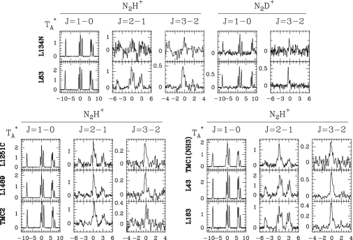
Figure 1.— Observed $J$=1–0, 2–1, and 3–2 transitions of N₂H⁺ in the direction of selected sources. Ordinate is antenna temperature and abscissa is the V_LSR. For each transition the assigned frequency corresponds to the one of the strongest hyperfine component.

Figure 2.— Observed radial integrated intensity profiles of L1517B, L1498, L1489, L43, L63 and TMC2 compared to the models. Observational data are from Caselli et al. (2002) (obtained with the FCRAO antenna) and Tafalla et al. (2004) for L1498 and L1517B (30m, Pico Veleta). For each source, the solid lines refer to the emerging intensities of our modeling (see text). For L1517B, the solid line correspond to the density profile used in this work and the dashed one to the profile used in Tafalla et al. (2004).

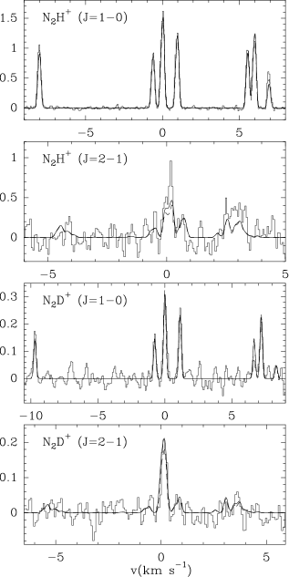
Figure 3.— Observed and modeled $J$=1–0 and 2–1 transitions of N₂H⁺ and N₂D⁺ towards L1517B. The solid line corresponds to the density profile used in this work and the dashed one corresponds to the profile used in Tafalla et al. (2004).

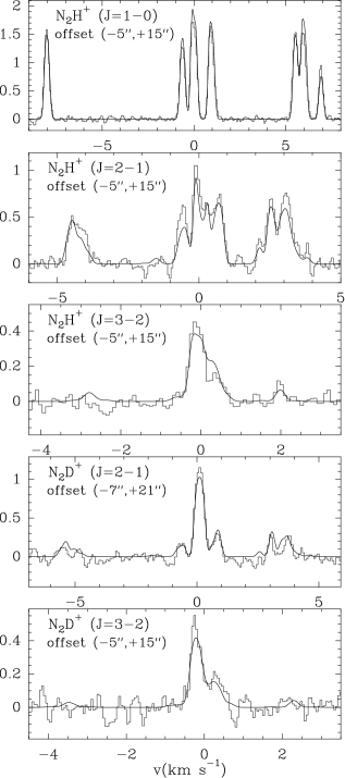
Figure 4.— Observed and modeled $J$=1–0, 2–1 and 3–2 lines of N₂H⁺ and $J$=2–1 and 3–2 lines of N₂D⁺ towards molecular peak C in L183.

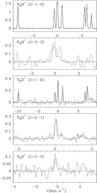
Figure 5.— Observed and modeled $J$=1–0 and 3–2 lines of N₂H⁺ and $J$=1–0, 2–1 and 3–2 lines of N₂D⁺ for the molecular peak N in L183.

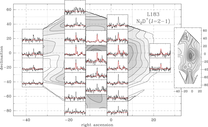
Figure 6.— Map and modeled lines of the $J$=2–1 transition of N₂D⁺ corresponding to molecular peak C in L183. The reference position of the map is reported in table 1 and corresponds to the N₂H⁺ and N₂D⁺ observations shown on figure 4. On the right side of the main map, the map of integrated intensity is reported with contour levels going from 20% to 90% of the map peak intensity, by step of 10%. Note that the aspect ratio between right ascension and declination is respected on the right map and show the South–North extent of the cloud.

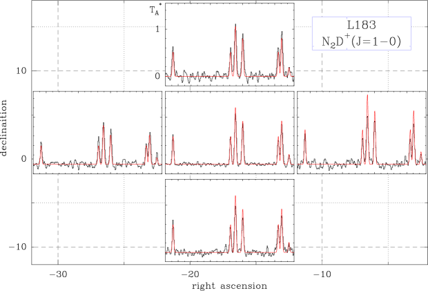
Figure 7.— Map and modeled lines of the $J$=1–0 transition of N₂D⁺ corresponding to the molecular peak C in L183.

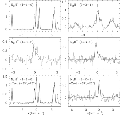
Figure 8.— Observed and modeled lines for two positions toward TMC2. At the position of the N₂H⁺ map peak are shown the $J$=1–0, 2–1 and 3–2 lines of N₂H⁺ and the $J$=3–2 line of N₂D⁺. For the offset position, are shown the $J$=1–0 line of N₂H⁺ and the $J$=2–1 line of N₂D⁺.

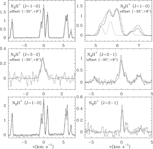
Figure 9.— Models for the $J$=1–0, 2–1 and 3–2 line of N₂H⁺ and for the $J$=3–2 line of N₂D⁺ observed in TMC1(NH₃). The upper right panel is a blow–up of the low frequency hyperfine triplet in the $J$=1–0 line, with the second emission component indicated.

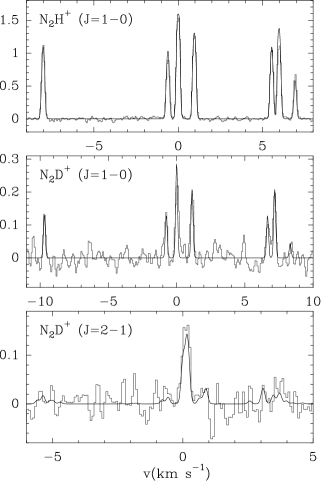
Figure 10.— Observed and modeled $J$=1–0 line of N₂H⁺, and the $J$=1–0 and 2–1 lines of N₂D⁺ towards L1498.

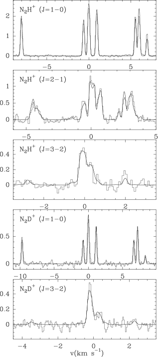
Figure 11.— Observed and modeled $J$=1–0, 2–1, and 3–2 lines of N₂H⁺ and $J$=1–0 and 3–2 lines of N₂D⁺ towards L63.

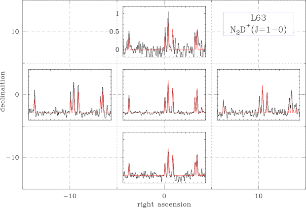
Figure 12.— Observed and modeled J=1–0 lines of N₂D⁺ for five position towards L63.

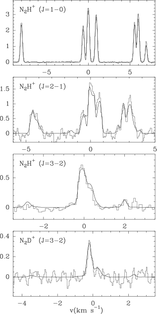
Figure 13.— Observed and modeled $J$=1–0, 2–1, and 3–2 lines of N₂H⁺ and $J$=3–2 line of N₂D⁺ towards L43.

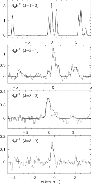
Figure 14.— Observed and modeled $J$=1–0, 2–1 and 3–2 lines of N₂H⁺ and $J$=3–2 line of N₂D⁺ towards L1489.

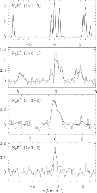
Figure 15.— Observed and modeled $J$=1–0, 2–1 and 3–2 lines of N₂H⁺ and $J$=3–2 line of N₂D⁺ towards L1251C.

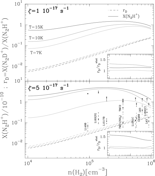
Figure 16.— N₂H⁺ fractional abundances (solid lines, in unit of 10^-10) and ratio of abundances $r_{D}$=X(N₂D⁺)/X(N₂H⁺) (dashed lines), for a cosmic ray constant of $\zeta=1\,10^{-17}$ s^-1 (upper panel) and $\zeta=5\,10^{-17}$ s^-1 (lower panel). For each panel, the results are shown for clouds at T = 7K (faint grey), T = 10K (grey) and T = 15K (black). The lower–right box of each panel compares the ratio $r_{D}$ to the ratio $r_{D}^{stat}$ predicted using equation 1. Central densities (n₀) , N₂H⁺ abundances, and abundance ratio ($R$) derived from models (see section 3) and listed in tables 2 and 3 are indicated in the lower panel, for comparison with the chemical models.

Figure 17.— $J$=1–0, 2–1 and 3–2 excitation temperature, opacity and brightness temperature of N₂D⁺ (dashed lines) and N₂H⁺ (solid lines) on the left column, and of HCO⁺ (solid lines), H¹³CO⁺ (dotted line) and DCO⁺ (long dashed) on the right column. The column density is the same for all molecules and is 10¹² cm^-2/(km s^-1 pc^-1).

Figure 18.— Comparison of excitation temperatures (left) and line intensity ratios (rigth) of ortho–H₂CO and para–D₂CO for different transitions of both species and a common column density of 10¹² cm^-2. Note that the quantum numbers of the selected transitions correspond to different symetries of the two isotopologues. Left panels show that excitation temperatures are different for both species for the range of densities found in dense cores.

References

- Aikawa et al. (2005) Aikawa Y., Herbst E., Roberts H. and Caselli P., 2005, ApJ, 620, 330
- Amano et al. (2005) Amano T., Hirao T., Takano J., 2005, J. Mol. Spectrosc., 234, 170
- Benson & Myers (1989) Benson P.J., Myers P.C., 1989, ApJ, 71, 89
- Butner et al. (1995) Butner H.M., Lada E.A., Loren R.B., ApJ, 448, 207
- Caselli et al. (1995) Caselli P., Myers P., Thaddeus P., 1995, ApJ, 455, L77
- Caselli et al. (2002) Caselli P., Benson P.J., Myers P., Tafalla M., 2002, ApJ, 572, 238
- Caselli et al. (2002b) Caselli P., Walmsley C.M., Zucconi A. et al., 2002b, ApJ, 565, 344
- Caselli et al. (2003) Caselli P., van der Tak F.F.S., Ceccarelli C., Bacmann A., 2003, A&A, 403, L37
- Cernicharo et al. (1984) Cernicharo J., Bachiller R., 1984, A&A, 58, 327
- Cernicharo (1985) Cernicharo J., IRAM internal report.
- Cernicharo et al. (1985) Cernicharo J., Bachiller R., Duvert G., A&A, 1985, 149, 273
- Crapsi et al. (2005) Crapsi A., Caselli P., Walmsley M., Myers P.C., Tafalla M., Lee C.W., Bourke T.L., 2005, ApJ, 619, 379
- Daniel et al. (2004) Daniel F., Dubernet M.–L. and Meuwly M., 2004, J. Chem. Phys., 121, 4540
- Daniel et al. (2005) Daniel F., Dubernet M.–L., Meuwly M., Cernicharo J., 2005, MNRAS, 363, 1083
- Daniel et al. (2006) Daniel F., Cernicharo J., Dubernet M.–L., 2006, ApJ, 648, 461
- Dickens et al. (2000) Dickens J.E., Irvine W.M., Snell R.L., Bergin E.A., Schloerb F.P., Pratap P. and Miralles M.P., 2000, ApJ, 542, 870
- Dore et al. (2004) Dore L., Caselli P., Beninati S., Bourke T., Myers P.C., Cazzoli, G., 2004, A&A, 413, 1177
- Flower et al. (2004) Flower D. R., Pineau des Forêts G. & Walmsley C.M. 2004, A&A, 427, 887
- Geppert et al. (2004) Geppert W. D., Thomas R., Semaniak J., Ehlerding A., Millar T. J., Osterdahl F., af Ugglas M., Djurić N., Paál A., Larsson M., 2004, ApJ, 609, 459
- Gerlich et al. (2002) Gerlich D., Herbst E. & Roueff E., 2002, Pl.Sp.Sc., 50, 1275
- Gerlich & Schlemmer (2002) Gerlich D. & Schlemmer S., 2002, Pl.Sp.Sc., 50, 1287
- Juvela et al. (2002) Juvela M., Mattila K., Lethinen K., Lemke D., Laureijs R. and Prusti T., 2002, A.&A., 382, 583
- Hirahara et al. (1992) Hirahara Y., Suzuki H., Yamamoto S., Kawaguchi K., Kaifu N., Onishi M., Takano S., Ishikawa S. and Masuda A., 1992, ApJ., 394, 539
- Langer et al. (1995) Langer W.D., Velusamy T., Kuiper T.B.H., Levin S., Olsen E. and Migenes V., 1995, ApJ, 453, 293
- Langer et al. (2001) Langer W.D. and Willacy K., 2001, ApJ, 557, 714
- Lique et al. (2006) Lique F., Cernicharo J., Cox J.–P., 2006, ApJ, 653, 1342
- Kirk et al. (2005) Kirk J.M., Ward–Thompson D., André P., 2005, MNRAS, 360, 1506
- Molek et al. (2007) Molek C.D., McLain J.L., Poterya V., N. G. Adams N.G., 2007, in preparation
- Monteiro (1985) Monteiro T.S., 1985, MNRAS, 214, 419
- Myers et al. (1979) Myers P.C., Ho P.T.P., Benson P.J., 1979, ApJ, 233, L141
- Olano et al. (1988) Olano C.A., Walmsley C.M. and Wilson T.L., 1988, A.&A., 196, 194
- Onishi et al. (1996) Onishi T., Mizuno A., Kawamura A., Ogawa H., Fukui Y., 1996, ApJ, 465, 815
- Onishi et al. (2002) Onishi T., Mizuno A., Kawamura A., Tachihara., Fukui Y., 2002, ApJ, 575, 950
- Pagani et al. (2003) Pagani L., Lagache G., Bacmann A., Motte F., Cambrésy L., Fich M., Teyssier D., Miville–Deschênes M.–A., J.–R. Pardo, Apponi A.J., Stepnik B., 2003, A&A, 406, L59
- Pagani et al. (2005) Pagani L., Pardo J.–R., Apponi A.J., Bacmann A., and Cabrit S., 2005, A&A, 429, 181
- Pagani et al. (2007) Pagani L., Bacmann A., Cabrit S., Vastel C., 2007, A&A, 467, 179
- Pardo et al. (2001) Pardo J.R., Cernicharo J., Serabyn G, 2001, IEEE Transactions on Antennas and Propagation, 49, 1683
- Parise et al. (2004) Parise B., Castets A., Herbst E., Caux E., Ceccarelli C., Mukhopadhyay I., Tielens A.G.G.M., 2004, 416, 159
- Parise et al. (2002) Parise B., Ceccarelli C., Tielens A.G.G.M., Herbst E., Lefloch B., Caux E., Castets A., Mukhopadhyay I., Pagani L., Loinard L., 2002, 393, 49
- Pratap et al. (1997) Pratap P., Dickens J.E., Snell R.L., Miralles M.P., Bergin E.A., Irvine W.M. and Schloerb F.P., 1997, ApJ, 486, 862
- Ramanlal & Tennyson (2004) Ramanlal J. ,Tennyson J., 2004, MNRAS, 354, 161
- Roberts et al. (2003) Roberts H., Herbst E. and Millar T.J., 2003, ApJ, 591, L41
- Roberts et al. (2004) Roberts H., Herbst E., Millar T. J., 2004, A&A, 424, 905
- Roberts & Millar (2000) Roberts H. & Millar T.J., 2000, A&A, 361, 388
- Roueff et al. (2005) Roueff E., Lis D., van der Tak F., Gerin M., Goldsmith P.F., 2005, A&A, 438, 585
- Roueff et al. (2000) Roueff E., Tiné S., Coudert L.H. et al., 2000, A&A, 354, L63
- Sato et al. (1992) Sato F., Mizuno A., Nagahama T., Onishi T., Yonekura Y. and Fukui Y., 1994, ApJ, 435, 279
- Shirley et al. (2005) Shirley Y.L., Nordhaus M.K., Grcevich J.M., Evans N.J., Rawlings J.M.C., and Tatematsu K., 2005, ApJ, 632, 982
- Snell (1981) Snell R.L., 1981, Ap. J. Suppl, 45, 121
- Tafalla et al. (2004) Tafalla M., Myers P.C., Caselli P., Walmsley C.M., 2004, A.&A., 416, 191
- Tiné et al. (2000) Tiné S., Roueff E., Falgarone E., Gerin M., Pineau des Forêts G., 2000, A.&A., 356, 1039
- Tóth et al. (1996) Tóth L.V., Walmsley C.M., 1996, A&A, 311, 981
- Tóth et al. (2004) Tóth L.V., Haas M., Lemke D., Mattila K. and Onishi T., 2004, A&A, 420, 533
- Tölle et al. (1981) Tölle F., Ungerechts H., Walmsley C.M., Winnewisser G. and Churchwell E., 1981, A.&A., 95, 143
- Vastel et al. (2004) Vastel C., Phillips T.G., Yoshida H., 2004, ApJ, 606, L127
- Vastel et al. (2006) Vastel C., Phillips T.G., Yoshida H., 2006, Astro-ph 06
- Walmsley et al. (2004) Wamsley C.M., Flower D.R., Pineau des Forêts G., 2004, A&A 418, 1035
- Walsh et al. (1998) Walsh M.S., Xu L.-H. and Lees R. M., 1998, J. Mol. Spectrosc., 188, 85
- Watson (1974) Watson W.D., 1974, ApJ, 188, 35
- Ward–Thompson et al. (1994) Ward–Thompson D., Scott P.F., Hills R.E., André P., 1994, MNRAS, 268, 276
- Ward–Thompson et al. (1999) Ward–Thompson D., Motte F. and André P., 1999, MNRAS, 305, 143
- Young et al. (2004) Young K.E., Lee J.–E., Evans N.J., Goldsmith P.F., Doty S.D., 2004, ApJ, 614, 252