Abstract

In this paper, bound states energies and corresponding wave functions of H-shaped quantum wires are calculated numerically in the presence of external magnetic and electric fields and within the Landau gauge. With a suitable definition of external confinement potential, we present a numerical algorithm to calculate the profile of probability distribution of charge carriers. Our analysis shows that in the presence of external electric and magnetic fields, bound state properties of carriers are sensitive functions of an asymmetric parameter $a=\frac{W_{x}}{W_{y}}$ which measures the relative width of the well in two directions. We also study many body effect of bandgap renormalization in this quasi one dimensional system within dynamical random phase approximation.
PACS: 73.20.Dx; 71.35.Ee; 71.45.Gm
Key Words: Quantum Wires, H-Shaped Confinement Potential, Bound States, Landau Gauge, Bandgap Renormalization

1 Introduction

A highly dense electron-hole plasma can be generated in a wide variety of semiconductors by optical pumping. The band structure and the optical properties of highly excited semiconductors generally differ from those calculated for non-interacting electron-hole pairs due to many-body exchange-correlation effects arising from the electron-hole plasma[1,2]. In recent years, quasi-one dimensional semiconductor quantum wires (QW) have been fabricated in a variety of geometric shapes with atomic scale definition, and QW optical properties have been studied for their potential device applications such as semiconductor lasers[3,4]. Recently different geometries of quantum wires, such as rectangular, V-shaped, L-shaped and T-shaped quantum wires have been fabricated and some of their electronic properties have been studied[4]. In addition, various experimental techniques for fabrication and growth of these structures have been developed[3-5]. Square quantum well wires have been studied by Hu and Das Sarma[6]. They have calculated the value of the band gap re-normalization( renormalization of fundamental gap structure due to many body exchange-correlation effects) for this case within GW approximation. Excitonic effects in quantum wires have been studied by Goldoni et al [7]. They have studied the effects of Coulomb interaction on the linear and nonlinear optical properties of both V-shaped and T-shaped semiconductor quantum wires. Wang and Das Sarma have proposed an elegant framework for numerical studies of carrier induced many-body effects on the excitonic optical properties of highly photoexcited one-dimensional quantum wire systems[8,9]. Hwang and Das Sarma have investigated the dynamical self-energy corrections of electron-hole plasma due to electron-electron and electron-phonon interactions at the band edges of a quasi-one dimensional photoexcited electron-hole plasma within GW approximation[10,11]. Rinaldi and Cingolani have studied the optical properties of quasi one dimensional quantum structures specially the case of V-shaped quantum wires[12]. Bener and Haug have considered plasma-density dependence of the optical spectra for quasi-one-dimensional quantum well wires[13]. Tanatar has studied the band gap re-normalization in quasi-one dimensional systems in a simple plasmon-pole (quasi-static) approximation[14,15]. Güven et al have studied the band-gap renormalization in quantum wire system within dynamical correlations and multi-subband effects[16]. Luttinger liquid behavior of a semiconductor quantum wire has been studied by Bellucci and Onorato[17]. They have also studied the effects of magnetic field on low dimensional electron systems focusing on Luttinger liquid behavior in a quantum wire[18]. In addition, they have studied also the ballistic electron transport in a quantum wire under the action of an electric field[19] and quenching of the spin Hall effect in ballistic nanojunctions[20]. As an application, recently they have studied the transport through a double barrier in large radius Carbon Nanotube with transverse magnetic field[21]. Many particle aspects of a semiconductor quantum wire within an improved random phase approximation has been studied by Ashraf and Sharma[22]. They have considered structure factor, pair distribution function, screened impurity potential and density of screening charge and exchange and screened exchange energies within an improved random phase approximation.

On the other hand, T-shaped and L-shaped quantum wires have been studied by some authors recently. For example, Sedlmaier and his coworkers have studied the band gap re-normalization of modulation doped T-shaped quantum wires. They have presented a self-consistent electronic structure calculation for this device[23]. Using a density functional theory, Stopa has calculated the electronic structure of a modulation doped and gated T-shaped quantum wire [24]. Szymanska et al have studied the excitons in T-shaped quantum wires[25]. They have calculated energies and oscillator strength for radiative recombination and two particle wave functions for ground state exciton in a T-shaped quantum wire. Lin, Chen and Chuu have found the dependence of the bound states of L-shaped and T-shaped quantum wires to some asymmetric parameter in an inhomogeneous magnetic field[26]. They have proposed a simple model to explain the behavior of the magnetic dependence of the bound state energy both in week and strong field regions. Recently Nozari and Madadi have studied numerically the bound states properties and the band gap renormalization of V-shaped and T-Shaped quantum wires within dynamical random phase approximation[27,28]. Ballistic transport through coupled T-shaped quantum wires has been studied by Lin et al [29].

As another possible geometry of low dimensional systems, H-shaped electronic systems have been considered and their many-body electronic properties have been studied by some authors. Shin and coworkers have studied quantum transport in an H-shaped quantum wire and a ring structure[30]. They have studied numerically the transport properties of an H-shaped quantum wire structure by using the mode matching technique. They have reported the existence of anomalous Hall resistance plateaus in this structure with relatively low magnetic fields as precursors of integer Hall plateaus. Henkiewicz et al have studied the manifestation of the spin Hall effect in a two-dimensional electronic system with Rashba spin-orbit coupling via dc-transport measurements in a realistic H-shaped structure[31]. Designing of H-shaped micromechanical structure has been studied by Arhaug and Soeraasen[32]. Our investigation shows that there is no other concrete study of these structure in existing literature. Obviously an analytical-numerical study of this special structure is important to fill the existing gap. Specially, our investigation of literature shows that bound states of H-shaped quantum wires and many-body effects such as bandgap renormalization of these low dimensional systems have not been studied yet. So, in this paper we consider the geometry of H-shaped quantum wires and by a suitable analytical definition of quasi-one dimensional H-shaped confinement potential, we propose a numerical scheme for calculating the bound states energies and wave functions of charge carriers in the presence of external electric and magnetic fields and within the Landau gauge. We obtain the profile of charge carriers distribution(probability distribution) in the presence of electric and magnetic fields. As an important nonlinear optical effect, the many-body exchange-correlation induced band gap narrowing in this type of quantum wire will be studied within leading order dynamical random phase approximation.

The paper is organized as follows: section $2$ is devoted to formulation of the problem and definition of confinement potential analytically. In section $3$ we give a short but complete review of bandgap renormalization in a general quasi-one dimensional semiconductor. Some numerical details are given at the end of this section. Section $4$ provides numerical results of our study and their interpretation, while the numerical scheme of our calculations based on finite difference algorithm is presented in the Appendix. The results of each step are shown by figures. Finally, summary and conclusions are given in section $5$.

2 The Setup

The geometry of a typical H-shaped quantum wire is shown in figure $1$. The typical values of $W_{x}$ and $W_{y}$ are of the order of $5-50$ Nanometer. We study bound states and many-body effects in this quasi one dimensional system in the presence of external electric and magnetic fields. The electric field is assumed to be directed along the $x$-axis and its typical value is of the order of a few $V/cm$. The presence of magnetic field is in such a way that the Landau gauge, $\vec{A}=(0,\,Bx,\,0)$ is satisfied. The Hamiltonian of an electron in this configuration can be written as follows

$$H=\frac{1}{2m}\Big{[}p_{x}^{2}+(p_{y}-eBx)^{2}\Big{]}-eEx$$ (1)

where $e$ and $m$ are electron charge and mass respectively. The Schrödinger equation of this electron with wave function $\Psi(x,y)$ can be written as follows

$$-\Bigg{(}\frac{\partial^{2}}{\partial x^{2}}+\frac{\partial^{2}}{\partial y^{2}}-\frac{2ieB}{\hbar}x\frac{\partial}{\partial y}\Bigg{)}\Psi(x,y)+\Bigg{(}\frac{eB}{\hbar}\Bigg{)}^{2}x^{2}\Psi(x,y)-\frac{2meE}{\hbar^{2}}x\Psi(x,y)=\frac{2m}{\hbar^{2}}\lambda\Psi(x,y)$$ (2)

where $\lambda$ stands for eigenvalues of energy, $E$ represents the value of electric field and $B$ is the value of the magnetic field. To solve this eigenvalue problem we need the boundary conditions which are given by the external confinement potential. The geometry of H-shaped quantum wire as shown in figure $1$, suggests the following definition of confinement potential

$$V(x,y)=\left\{\begin{array}[]{ll}0&{\rm if}\left\{\begin{array}[]{ll}-\infty<x<+\infty,\quad-\frac{3}{2}W_{y}\leq y\leq-W_{y}\\ -\infty<x<+\infty,\quad W_{y}\leq y\leq\frac{3}{2}W_{y}\\ -\frac{W_{x}}{2}\leq x\leq\frac{W_{x}}{2},\quad-W_{y}\leq y\leq W_{y}\end{array}\right.\\ \newline \infty&{\rm elsewhere}\end{array}\right.$$ (3)

With this definition of confinement potential (which provides the required boundary conditions), we solve equation (2) numerically to find eigenvalues and eigenfunctions of bound states of electron in the presence of electric and magnetic fields. Our numerical strategy based on finite difference algorithm is presented in the Appendix. The results of these calculations for different external field configurations and variety of possibilities are shown in Figures and will be interpreted in section $4$. The bound states wave functions obtained in this section will be used to study the bandgap renormalization of H-shaped quantum wire in the next section.

3 Many Body Effects in H-Shaped Quantum Wires

There are several nonlinear optical many body effects in quasi-one dimensional semiconductor systems originating from exchange-correlation effects in a dense excited plasma. One of the most important many-body effect in high density electron-hole plasma is a density-dependent re-normalization of the fundamental band gap of the semiconductor, which causes an increasing absorption in the spectral region below the lowest exciton resonance. The exchange-correlation correction of the fundamental band gap due to the presence of free carriers (electrons in the conduction band and holes in the valence band) in the system is referred to as the band gap re-normalization effect. Optical nonlinearities, which are strongly influenced by screened Coulomb interaction in the electron-hole plasma, are typically associated with the band gap re-normalization phenomenon. In which follows we use the two band(one conduction band and one valance band) model to study the one dimensional electron-hole system. We neglect the effects of higher subbands and degeneracies in valance bands. We assume that electrons and holes densities are constant in time. In this situation, Hamiltonian of the system can be written as[8,9,33]

$$H=\sum_{k}\Bigg{[}\bigg{(}E^{0}_{g}+\frac{k^{2}}{2m_{e}}c^{{\dagger}}_{k}c_{k}+\frac{k^{2}}{2m_{h}}d^{{\dagger}}_{k}d_{k}\bigg{)}\Bigg{]}$$

$$+\frac{1}{2L}\sum_{k,k^{\prime},q}\bigg{[}V_{c,ee}(q)c^{{\dagger}}_{k-q}c^{{\dagger}}_{k^{\prime}+q}c_{k^{\prime}}c_{k}+V_{c,hh}(q)d^{{\dagger}}_{k-q}d^{{\dagger}}_{k^{\prime}+q}d_{k^{\prime}}d_{k}+V_{c,eh}(q)c^{{\dagger}}_{k-q}c_{k}d^{{\dagger}}_{k^{\prime}+q}d_{k^{\prime}}\bigg{]}.$$ (4)

In this equation which contains all information about this one dimensional system, $c_{k}$ and $c^{{\dagger}}_{k}$ are annihilation and creation operators for conduction electrons respectively. Also $d_{k}$ and $d^{{\dagger}}_{k}$ are annihilation and creation operators for valance band holes. $E^{0}_{g}$ is the direct band gap between the top of the valance band and the bottom of the conduction band. $V_{c,ij}$ show the possible three Coulomb interactions between electrons and holes. Note that the two first interactions lead to electron-hole quasi particle self-energies while the third one leads to the production of excitonic bound states. Note also that this Hamiltonian consists of spin effects, although spin index is not included explicitly.

The Coulomb interaction matrix element in one dimensional quantum wire is given by the following relation[8]

$$V_{c,ij}(q)=\frac{e^{2}}{\epsilon_{0}}\int_{-\infty}^{+\infty}dxdx^{\prime}\int_{-\infty}^{+\infty}dydy^{\prime}\int_{-\infty}^{+\infty}dz\frac{e^{-iqz}|\phi_{i}(x,y)|^{2}|\phi_{j}(x^{\prime},y^{\prime})|^{2}}{\sqrt{z^{2}+(y-y^{\prime})^{2}+(x-x^{\prime})^{2}}}$$

$$=\frac{2e^{2}}{\epsilon_{0}}\int_{-\infty}^{+\infty}dxdx^{\prime}\int_{-\infty}^{+\infty}dydy^{\prime}|\phi_{i}(x,y)|^{2}|\phi_{j}(x^{\prime},y^{\prime})|^{2}K_{0}\Big{(}q\sqrt{(x-x^{\prime})^{2}+(y-y^{\prime})^{2}}\Big{)},$$ (5)

where $\phi_{i}(x,y)$ is the quantum wire confinement wave function for the lowest eigenstate of electrons or holes. The exact form of these eignfunctions depends on the geometry and details of confinement potential. $K_{0}(x)$ is the zeroth-order modified Bessel function of second kind. In the setup of our one dimensional quantum system we have assumed that carriers are free to move in $z$ direction but $x$ and $y$ are directions of confinement.

Band gap renormalization in quasi-static approximation is given by[14,15]

$$\Delta_{i}(k)=\sum_{k^{\prime}}\Big{[}-V_{s}(k-k^{\prime})n_{i}(\varepsilon_{i,k})+\frac{1}{2}(V_{s}(k^{\prime})-V_{c}(k^{\prime}))\Big{]}$$ (6)

where

$$V_{s}(k)\equiv V_{s}(k,\omega=0)=\frac{V_{c}(k)}{\varepsilon(k,\omega=0)}$$ (7)

is the statically screened Coulomb interaction and $n_{i}(\varepsilon_{i,k})$ is the fermion momentum distribution function

$$n_{i}(\varepsilon_{i,k})\equiv(e^{\beta(\varepsilon_{i,k}-\mu_{i})}+1)^{-1}$$ (8)

where $\varepsilon_{e,k}\equiv\frac{k^{2}}{2m_{e}}+E^{0}_{g}$ and $\varepsilon_{h,k}\equiv\frac{k^{2}}{2m_{h}}$ are the bare energies of electron and hole in their respective bands and $\mu_{i}$ is the chemical potential. $\varepsilon(k,\omega)$ as dynamical dielectric function is defined as follows

$$\varepsilon(k,\omega)=1-V_{c}(k)\Pi^{0}_{e}(k,\omega)-V_{c}(k)\Pi^{0}_{h}(k,\omega)=1-V_{c}(k)\sum_{i=e,h}\frac{m_{i}}{\pi k}\ln\bigg{[}\frac{\omega^{2}-[(k^{2}/2m_{i})-k\upsilon_{F,i}]^{2}}{\omega^{2}-[(k^{2}/2m_{i})+k\upsilon_{F,i}]^{2}}\bigg{]}$$ (9)

where $\upsilon_{F,e/h}$ is the Fermi velocity of electrons/holes at Fermi momentum in the conduction/valance band.

In one-loop GW approximation with dynamically screened interaction, one has[8,33]

$$\Sigma_{i}(k,z)=-\frac{1}{\beta}\sum_{k^{\prime},z^{\prime}}V_{s}(k-k^{\prime},z-z^{\prime})G_{i}(k^{\prime},z^{\prime})=-\frac{1}{\beta}\sum_{k^{\prime},z^{\prime}}\frac{V_{c}(k-k^{\prime})}{\varepsilon(k-k^{\prime},z-z^{\prime})}G_{i}(k^{\prime},z^{\prime})$$ (10)

where

$$G_{i}(k,z)=\frac{1}{z-\varepsilon_{i,k}-\Sigma_{i}(k,z)+\mu_{i}},\quad\quad\quad(i=e,h)$$ (11)

and $\Sigma_{e/h}(k,z)$ is the self energy of electrons/holes defined in GW approximation. To avoid multi-pole structure in $G_{i}(k,z)$ we approximate $\Sigma_{i}(k,z)$ by momentum-dependent band gap renormalization $\Delta_{i}(k)$. Using the approximation $\Delta_{i}(k)=\Sigma_{i}(k,\varepsilon_{i,k}-\mu_{i})$, we find the following single pole electron-hole Green’s function[8,33]

$$G_{i}(k,z)\sim\frac{1}{z-\varepsilon_{i,k}-\Delta_{i}(k)+\mu_{i}},\quad\quad\quad(i=e,h)$$ (12)

The above formalism provides a suitable framework for our numerical calculation of band gap renormalization. To proceed further, we should calculate the screened coulomb potential. Using equation (5), it can be written as follows

$$V_{c}(k)=\frac{2e^{2}}{\varepsilon_{0}}\int dxdy\int dx^{\prime}dy^{\prime}K_{0}|kR||\Psi(x,y)|^{2}|\Psi(x^{\prime},y^{\prime})|^{2},$$

or using rescaled coordinates $\tilde{x_{i}}\equiv\frac{x_{i}}{L}$ and $\tilde{x_{i}}^{\prime}\equiv\frac{x_{i}^{\prime}}{L}$ we find

$$V_{c}(k)=\lambda\frac{2e^{2}}{\varepsilon_{0}}L^{4}\int d\tilde{x}d\tilde{y}\int d\tilde{x}^{\prime}d\tilde{y}^{\prime}K_{0}|kR||\Psi(\tilde{x},\tilde{y})|^{2}|\Psi(\tilde{x}^{\prime},\tilde{y}^{\prime})|^{2},$$ (13)

where $\lambda$ is re-scaling factor equal to $10^{-18}/m^{2}$ and $kR=k\sqrt{(x-x_{0})^{2}+(y-y_{0})^{2}}$. Using $\Psi(x,y)$ computed numerically in the previous section, we solve the integral of equation (13). The screened potential is calculated by ground state wave function as a function of k. Figure 15 shows the result of this calculation for different values of relative width of the confinement potential. In this figure, $V_{c}(k)$ is normalized by $\frac{2e^{2}}{\epsilon_{0}}$ and the $k$ is normalized to $kL$.
In the next step we calculate the band gap renormalization in both quasi static and GW approximation. To do this end, we should calculate some quantities numerically. Using the re-scaled quantities $\tilde{k}=kL$ and $\omega=\tilde{\omega}\times 10^{16}$, we write relation (9) as follows

$$\varepsilon(k,\omega)=1-V_{c}(k^{\prime})\Bigg{(}\frac{1.7\times 10^{45}}{\tilde{k}L}\ln\Bigg{[}\frac{\tilde{\omega}^{2}\times 10^{7}-525[12\frac{\tilde{k}^{2}}{L^{2}}-\frac{\tilde{k}}{L}]^{2}}{\tilde{\omega}^{2}\times 10^{7}-525[12\frac{\tilde{k}^{2}}{L^{2}}+\frac{\tilde{k}}{L}]^{2}}\Bigg{]}$$ (14)

$$+\frac{5.18\times 10^{44}}{\tilde{k}L}\ln\Bigg{[}\frac{\tilde{\omega}^{2}\times 10^{6}-174[43.8\frac{\tilde{k}^{2}}{L^{2}}-\frac{\tilde{k}}{L}]^{2}}{\tilde{\omega}^{2}\times 10^{6}-174[43.8\frac{\tilde{k}^{2}}{L^{2}}+\frac{\tilde{k}}{L}]^{2}}\Bigg{]}\Bigg{)}.$$ (15)

The single pole Green s function for electron defined as relation (12) transforms to the following form

$$G(k,z)=\frac{1}{1.06\times 10^{-26}i\tilde{\omega}-6.17\times 10^{-21}\frac{\tilde{k}^{2}}{L^{2}}-2.47\times 10^{-19}-\Delta_{e}(k)}$$ (16)

and Green s function for hole becomes

$$G(k,z)=\frac{1}{1.06\times 10^{-26}i\tilde{\omega}-9.2\times 10^{-20}\frac{\tilde{k}^{2}}{L^{2}}+1.6\times 10^{-22}-\Delta_{h}(k)}.$$ (17)

To calculate bandgap renormalization in this configuration, we define the re-scaled $\beta_{e}$ and $\mu_{e}^{0}$ respectively as $\frac{\beta\hbar^{2}}{2m_{e}^{*}W_{y}^{2}}=\beta\frac{574.5}{W_{y}^{2}}$ and $\mu^{0}_{e}\beta$, where $W_{y}$ is width of quantum well in $y$ direction in Nanometer. For holes, we also define the re-scaled $\beta_{h}$ and $\mu^{0}_{h}$ as $\beta_{h}=\beta_{e}\big{(}\frac{m^{*}_{e}}{m^{*}_{h}}\big{)}$ and $\mu_{h}^{0}=\mu_{e}^{0}\big{(}\frac{m^{*}_{e}}{m^{*}_{h}}\big{)}$ respectively. In all computations in this paper, we have assumed that the ratio $\frac{m_{h}^{*}}{m_{e}^{*}}$ is equal to $0.3$ and $m_{e}^{*}\simeq 0.067m_{e}$. Then we set $\tilde{\omega}=0$ and using equation (7), we calculate band gap renormalization in both quasi static and GW approximations at temperature $T=0$. The result of calculation for both quasi static and GW approximation is shown in figure 16. As this figure shows, the value of band gap renormalization in GW approximation is smaller than the quasi static plasmon-pole approximation. Typical values of band gap normalization are between 10-30 $meV$ depending on the temperature and impurities in the system. Because of consideration of more quantum field theory details, GW approximation generally gives results which have better agreement with experimental results[10,11].

4 Interpretation of Numerical Results and conclusions

Probability distribution of charge carriers in the absence of external electric and magnetic fields are shown in figure $2$ where the asymmetric parameter $a=\frac{W_{x}}{W_{y}}$ has been set equal to $0.8$. This figure emphasizes the central role played by geometric shape of the confinement potential. In another words, in the absence of external electric and magnetic fields, carrier distribution obeys the symmetry of confinement potential. Variation of asymmetric parameter changes the profile of charge distribution in such a way that the case with $a=1$ has maximum symmetry and any change of relative width leads to antisymmetric distribution. Figure $3$ shows the variation of the ground state energy of carrier versus the inverse of the asymmetric parameter $a$. Variation of the relative width leads to the conclusion that smaller relative width leads to smaller ground state energy. Now, suppose that we turn on a uniform magnetic field. In the absence of electric field the distribution of charge carriers is given by figure $4$. The role played by asymmetric parameter is a reduction of probability amplitude when the width of the well increases in $x$ or $y$ direction. Variation of ground state energy versus the intensity of magnetic field is depicted in figure $5$ for two different values of asymmetric parameter. For a fixed well width in $y$ direction, when the width of the well in $x$ direction increases the value of the ground state energy will increase.
Now we turn off magnetic field and apply a uniform electric field in the $x$ direction. The profile of probability amplitude for charge carriers distribution is shown in figure $6$ for $a=0.8$. The probability amplitude has a Gaussian profile and is shifted toward the right hand side. This shift is a function of electric field intensity. The probability profile does not obey the geometric shape of the confinement potential due to preferred direction defined by the presence of electric field. The energy of the ground state versus the intensity of electric field is depicted in figure $7$. As this figure shows, ground state energy decreases with increasing electric field intensity. This is not surprising since external electric field tends to decouple electrons and holes from each other. In the general case where both electric and magnetic fields are present, the asymmetric situation explained above will be enhanced in some respects. Figures $8$ shows the space variation of the probability amplitude with $a=0.8$. In the presence of constant electric and magnetic fields, pick of the graph describing charge carriers distribution will be shifted to the positive direction of the $x$ axis. This feature causes the carriers concentration in such a way that these carriers distribution do not obeys the external confinement potential symmetry. More the intensity of the electric field results in more shift of the distribution pick to the right hand side of the $x$ axis. The presence of constant magnetic field causes the anisotropy in the profile of the probability distribution of the carriers. Figure $9$ shows the variation of the ground state energy versus the variation of the electric field when the magnetic field is supposed to be constant. More intensity of the electric field leads to the more reduction of the bound states energies. This resembles the linear Stark effect in elementary quantum mechanics. In the language of many body effects in dense plasma in a quasi one dimensional semiconductor, application of intense electric field results in the weaker excitonic states. Therefore, the presence of external electric and magnetic fields will shift the location of maximum concentration of carriers and in this case there is an apparent asymmetry in profile of carriers distribution. This point can be used in fabrication of microelectronic devices based on quantum wires.

We have proposed a numerical framework to calculate screened Coulomb potential and the values of band gap energy re-normalization in H-shaped quantum wire in two different approximations: quasi-static and dynamical random phase approximation in its leading order dynamical screening (GW approximation). We have evaluated the single particle self-energies for both electrons and holes in the dynamical plasmon pole approximation (PPA) and the leading order dynamically screened interaction or GW approximation to obtain the electron and hole renormalized Green s functions. This self-energy calculation gives us the band gap renormalization due to exchange-correlation effect. For comparison, we also calculated the band gap renormalization obtained by the quasi static calculation in both static random phase approximation and static plasmon pole approximation. Note that quasi static approximation works well in two and three dimensional systems but fails completely in one dimensional systems. This is because the electrons in one dimensional system suffer very strong inelastic scattering effects by virtue of restricted phase space. However, we have used this approximation only for comparison purposes. It is important to note that by re-scaling procedure which we have considered, we have fixed the geometry of the H-shaped quantum wire. Actually, one should consider the possibility for changing the geometry also. This has been down by change in parameter $L$ but our calculations show that the main physical results do not change considerably.

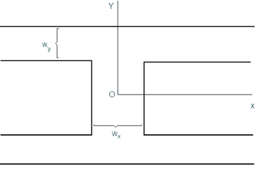
Figure 1: The Geometry of the H-Shaped Quantum Wire

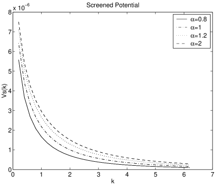
Figure 10: The calculated screened Coulomb potential versus the wave number for different asymmetry parameter. The screened potential is normalized by $\frac{2e^{2}}{\epsilon_{0}}$ and the $k$ is normalized by $L=W_{y}$.

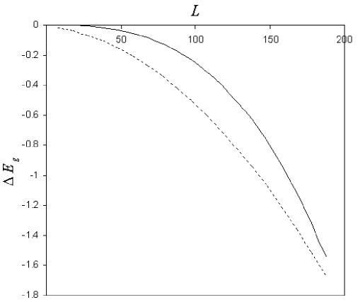
Figure 11: Calculated band gap renormalization in H-Shaped quantum wire within dynamical random phase(GW) approximation(upper curve) and quasi-static plasmon-pole approximation(lower curve). The screened potential is normalized by $\frac{2e^{2}}{\epsilon_{0}}$ and the $k$ is normalized by $L=W_{y}$.

Figure 10 shows the screened Coulomb potential calculated based on random phase approximation in its leading order and for different values of asymmetry parameter. Exchange-correlation many body effects mediate the bare Coulomb interaction. Based on different width of the confinement potential, screened Coulomb potential varies with geometrical characteristics of confinement potential. As the figure 10 shows, by increasing the asymmetry parameter, screened Coulomb potential will grows but its overall behaviors with respect to wave number will not change. Figure $10$ shows the calculated band gap renormalization in quasi static and dynamical random phase approximations. To calculate band gap renormalization we first calculate the electron/hole single pole Green’s function and then using the formalism of both one-loop GW approximation and quasi static plasmon pole approximation we calculate the values of band gap renormalization in $T=0$. Note that we have considered $L$ dependence of band gap renormalization, however it can be translated to band gap renormalization versus carrier densities as well. Figure 11 also compares the results of band gap renormalization in GW and plasmon-pole approximations. As this figure shows, for a fixed value of $L$, GW approximation gives smaller values of band gap renormalization. Generally GW approximation gives more reliable result in comparison with experimental data[5]. Note that we have focused on the variation of geometry by variation of $L$. As figure 1 shows there are other possibilities for changing the geometrical shape of external confinement potential. However the general behavior is the same as presented here. There are some restrictions on our calculations which can be summarized as follows: the many-body treatment has the disadvantage that, for band gap renormalization it commonly ignores geometrical factors, such as the quantum confined Stark effect, whose relevance is structure specific. In other words, the numerical results for different confinement potential of H-shaped quantum wire may be geometry dependent in general. Furthermore, in the exciton problem, many-body theory treats screening within the linear approximation and, generally, influence of the bound electron on the free electrons is not fully included. In particular the orthogonality of the free electron states with the bound state, which increases its importance in lower dimensional systems, are typically not included. On the other hand the complete treatment of the problem should consider the effects of several subbands[8]. Note that in the rest of the calculation of band gap renormalization we have used the two band(one conduction band and one valance band) model and we have neglected the effects of higher subbands and degeneracies in valance bands. We also assumed that electrons and holes densities are constant in time. In summary, many body effects in quasi one dimensional systems are sensitive to the geometrical shape of external confinement effects. The value of band gap renormalization in GW approximation is smaller than quasi static plasmon-pole approximation. Typical values of this normalization are between 10-30 $meV$ depending to temperature and impurities in the system. GW approximation generally gives results which have better agreement with experiment. A complete study of this problem requires the considerations of several subbands and varying electrons and holes densities.

5 Summary and Conclusions

Our numerical procedure to the bound states and many-body effects in H-shaped quantum wires has the following results:

• The distribution of the probability of the charge carriers in the ground state of the H-shaped quantum wire in the absence of electric and magnetic fields has a symmetric shape obeying the geometric shape of the confinement potential. This distribution has its maximum at the center of each arm and decreases with distance from the center. The relative width of the confinement potential(the asymmetric ratio $a=\frac{W_{x}}{W_{y}}$ has considerable effect on the profile of this distribution.

• In the presence of a constant magnetic field, the distribution of the charge carriers becomes oscillatory both in $x$ and $y$ directions. Increasing the strength of the magnetic field leads to the reduction of the ground state energy. The role played by the asymmetric parameter is given by the reduction of the probability amplitude when the width of the well increases in $x$ or $y$ directions.

• The situation for the case of non-vanishing electric field (in the absence of magnetic field) resembles the Stark effect in a low dimensional system. The probability amplitude has an oscillatory behavior with larger wavelength of the oscillations. In this case although the probability amplitude has a Gaussian profile, it is shifted toward the right hand side. This shift is a function of the electric field intensity. The probability profile does not obey the symmetry of the geometric shape of the confinement potential due to preferred direction defined by the presence of the electric field.

• In the presence of both electric and magnetic fields there are oscillations in probability distribution both in $x$ and $y$ directions, but in this case the probability distribution is not symmetric. In the presence of constant electric and magnetic fields, the pick of the probability amplitude will be shifted along the positive direction of the $x$ axis. This causes the carriers to be concentrated in such a way that they do not obey the external confinement potential symmetry. More intensity of the electric field results in more shift of the distribution pick to the right hand side of the $x$ axis. The presence of constant magnetic field causes an anisotropy in the profile of the probability distribution of the carriers since it apparently breaks the local rotational symmetry in the center of each arm.

• Screened Coulomb potential of the H-shaped external confinement is a sensitive function of the asymmetry parameter but its general behavior under variation of wave number is the same for other possible geometries of quasi one dimensional systems. The calculated band gap narrowing for H-shaped confinement potential in the absence of the electric and magnetic fields and within quasi-static and dynamical random phase approximation shows a typical gap narrowing of the order of few $meV$. This is supported from other studies of band gap narrowing in quasi one dimensional semiconductor systems[4,6]. The dynamical random phase approximation leads to more reliable result than quasi static approximation in comparison with experiments.

In summary we can conclude that in the presence of electric and magnetic fields, H-shaped quantum wires bound states characteristics are sensitive functions of an asymmetric parameter $a=\frac{W_{x}}{W_{y}}$ and the strength of the electric and magnetic fields. The case of non-vanishing electric and magnetic fields induces an intrinsic inhomogeneity in the quasi one dimensional system. Many-body effects due to plasma screening and resulting optical nonlinearities are also dependent to the asymmetric parameter of quasi-one dimensional confinement potential. Among these nonlinear optical effects, band gap renormalization of fundamental band age has been studied numerically in this paper.

Appendix: Numerical Strategy

We use the finite difference algorithm[34] to solve our partial differential equation(2) with boundary conditions imposed by H-shaped confinement potential. The most straightforward refinement method replaces the differential equation with a finite difference equation. It replaces all derivatives with approximate expression as the following familiar form

$$\Bigg{(}\frac{dy}{dx}\Bigg{)}_{x=x_{n}}\approx\frac{y_{n+1}-y_{n}}{h}$$

$$\Bigg{(}\frac{d^{2}y}{dx^{2}}\Bigg{)}_{x=x_{n}}\approx\frac{y_{n+1}-2y_{n}+y_{n-1}}{h^{2}}$$ (18)

where the mesh chosen to be equally spaced and given by   $h=\frac{x_{k}-x_{0}}{N+1}$  with $x_{k}=x_{0}+kh$ and $k=1,\,2,\,...,n+1$. We first re-scale the Schrödinger equation and the confinement potential. We define the re-scaled value of $x$ and $y$ as $\bar{x}\equiv\frac{x}{W_{x}}$ and $\bar{y}\equiv\frac{y}{W_{y}}$ where $W_{x}$ and $W_{y}$ are the width of the well in $x$ and $y$ direction respectively. Now the re-scaled Schrödinger equation can be written as follows

$$-\Bigg{(}\frac{1}{W_{x}}\frac{\partial^{2}}{\partial\bar{x}^{2}}+\frac{1}{W_{y}}\frac{\partial^{2}}{\partial\bar{y}^{2}}-\frac{2ieBW_{x}}{\hbar W_{y}}\bar{x}\frac{\partial}{\partial\bar{y}}\Bigg{)}\Psi(\bar{x},\bar{y})+\Bigg{(}\frac{eBW_{x}}{\hbar}\Bigg{)}^{2}\bar{x}^{2}\Psi(\bar{x},\bar{y})$$

$$-\frac{2meEW_{x}}{\hbar^{2}}\bar{x}\Psi(\bar{x},\bar{y})=\frac{2m}{\hbar^{2}}\lambda\Psi(\bar{x},\bar{y}).$$ (19)

Using the finite difference algorithm, this equation can be written as follows

$$-\Bigg{(}\frac{\Psi_{i+1,j}-2\Psi_{i,j}+\Psi_{i-1,j}}{\Delta_{x}}+a^{2}\frac{\Psi_{i,j+1}-2\Psi_{i,j}+\Psi_{i,j-1}}{\Delta_{y}}\Bigg{)}$$

$$+\frac{2ieaBW_{x}^{2}}{\hbar}\bar{x_{i}}\frac{\Psi_{i,j+1}-\Psi_{i,j-1}}{2\Delta_{y}}+\Bigg{(}\frac{eBW_{x}^{2}}{\hbar}\Bigg{)}^{2}\bar{x_{i}}^{2}\Psi_{i,j}-\frac{2meEW_{x}^{3}}{\hbar^{2}}\bar{x_{i}}\Psi_{i,j}=\frac{2mW_{x}^{2}}{\hbar^{2}}\lambda\Psi_{i,j}.$$ (20)

where $a=\frac{W_{x}}{W_{y}}$ is the relative width of the H-shaped quantum wire. We do discritize the $x$  and  $y$ axes to discrete space $dx=0.1$   and   $dy=0.1$, therefore the equation (20) can be written as a matrix equation

$${\cal H}\phi=E\phi,$$ (21)

where $\cal H$, and $\phi$ are the Hamiltonian matrix and the state wave functions array which are defined as follows

$$\phi=\left(\begin{array}[]{c}\left(\vdots\right)\\ \left(\begin{array}[]{c}\vdots\\ \phi(x_{i},y_{j})\\ \phi(x_{i+1},y_{j})\\ \vdots\end{array}\right)\\ \left(\begin{array}[]{c}\vdots\\ \phi(x_{i},y_{j+1})\\ \phi(x_{i+1},y_{j+1})\\ \vdots\end{array}\right)\\ \left(\vdots\right)\end{array}\right)$$ (34)

$${\cal H}=\left(\begin{array}[]{cccc}\left(\ddots\right)&\left(\begin{array}[]{ccc}\ddots&0&0\\ 0&-\frac{a^{2}}{\Delta_{y}^{2}}+\frac{iW_{x}eaB\bar{x_{i}}}{\hbar}&0\\ 0&0&\ddots\end{array}\right)&0&0\\ \left(\ddots\right)&\left(\begin{array}[]{cccc}\ddots&\ddots&0&0\\ \ddots&2(\frac{1}{\Delta_{x}^{2}}+\frac{a^{2}}{\Delta_{y}^{2}})+(\frac{eW_{x}^{2}B}{\hbar})^{2}\bar{x_{i}}^{2}+\frac{2meW_{x}^{3}E}{\hbar^{2}}\bar{x_{i}}&\frac{-1}{\Delta_{x}^{2}}&0\\ 0&\frac{-1}{\Delta_{x}^{2}}&2(\frac{1}{\Delta_{x}^{2}}+\frac{a^{2}}{\Delta_{y}^{2}})+(\frac{eW_{x}^{2}B}{\hbar})^{2}\bar{x_{i}}^{2}+\frac{2meW_{x}^{3}E}{\hbar^{2}}\bar{x_{i}}&\ddots\\ 0&0&\ddots&\ddots\end{array}\right)&\left(\ddots\right)&0\\ 0&\left(\begin{array}[]{ccc}\ddots&0&0\\ 0&-\frac{a^{2}}{\Delta_{y}^{2}}-\frac{iW_{x}eaB\bar{x_{i}}}{\hbar}&0\\ 0&0&\ddots\end{array}\right)&\left(\ddots\right)&\left(\ddots\right)\\ 0&0&\left(\ddots\right)&\left(\ddots\right)\end{array}\right)$$ (49)

The error of computation of $\phi(x,y)$ is of the order of $O(dx^{2})$. We diagonalize the Hamiltonian matrix and calculate the bound states energies and wave functions numerically. We use MATLAB package since it uses techniques that are more efficient than Jacobi rotations and that can be applied to asymmetric or even complex matrices as well as to the more common real symmetric situations.

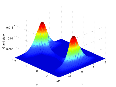
Figure 2: The probability amplitude of charge carriers distribution for ground state of H-shaped quantum wire at zero external EM fields. The asymmetry parameter has been chosen to be $a=\frac{W_{x}}{W_{y}}=0.8$.

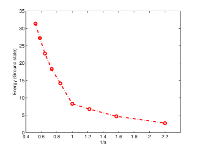
Figure 3: The ground state energy versus the inverse of the asymmetry parameter at zero external fields strength.

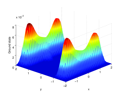
Figure 4: The probability amplitude of charge carriers distribution for ground state of H-shaped quantum wire in the presence of an external magnetic field(and zero electric field). The asymmetry parameter has been chosen to be $a=\frac{W_{x}}{W_{y}}=0.8$.

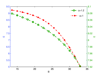
Figure 5: The ground state energy versus the intensity of the external magnetic field for different values of asymmetry parameter.

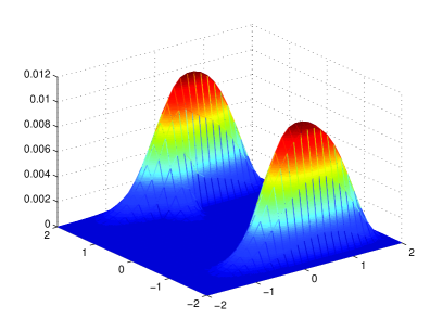
Figure 6: The probability amplitude of charge carriers distribution for ground state of H-shaped quantum wire in the presence of an external electric field(and zero magnetic field). The asymmetry parameter has been chosen to be $a=0.8$.

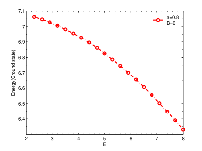
Figure 7: The ground state energy versus the intensity of the external electric field for $a=0.8$ and $B=0$.

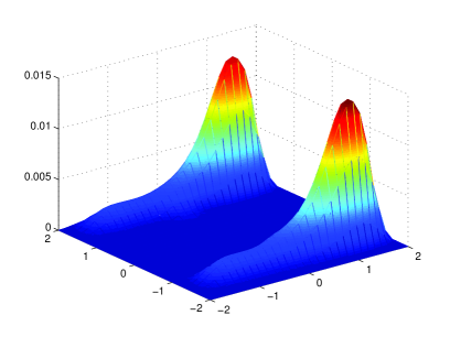
Figure 8: The probability amplitude of charge carriers distribution for ground state of H-shaped quantum wire in the presence of both electric and magnetic fields. The asymmetry parameter has been chosen to be $a=0.8$.

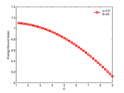
Figure 9: The ground state energy versus the intensity of the external electric field for $a=0.8$ and $B=20$ (a constant magnetic field).

References

- [1] N. Peyghambarian, S. W. Koch and A. Mysyrowicz, Introduction to Semiconductor Optics, Prentice Hall, 1993
- [2] H. Haug and S. W. Koch, Quantum Theory of the Optical and Electronic Properties of Semiconductors, World Scientific, Singapore, 1993.
- [3] V. V. Mitin, V. A. Kochelap and M. A. Stroscio,Quantum Hetrostructures: Microelectronics and Optoelectronics, Cambridge University Press, 1999
- [4] P. Harrison, Quantum Wells, Wires and Dots, John Wiley and Sons,2000.
- [5] H. Kalt, Optical Properties of III-V Semiconductors, Springer-Verlag, Berlin, 1996
- [6] B. Y. Hu and S. Das Sarma, Phys. Rev. B 48 (1993) 5469
- [7] G. Goldoni, F. Rossi and E. Molinari, Phys. Rev. B 55 (1996) 7110
- [8] D. W. Wang and S. Das Sarma, Phys. Rev. B 64 (2001) 195313
- [9] S. Das Sarma and D. W. Wang, Phys. Rev. Lett. 84 (2000) 2010
- [10] E. H. Hwang and S. Das Sarma, Phys. Rev. B 58 (1998) R1738
- [11] S. Das Sarma and E. H. Hwang, Phys. Rev. B 59 (1999) 10730
- [12] R. Rinaldi and R. Cingolani,Optical Spectroscopy of Low Dimensional Semiconductors Editted by G. Abstreiter and et al., Kluwer Academic Publishers, 1997
- [13] S. Benner and H. Haug, Europhys. Lett. 16 (1991) 579 and Phys. Rev. B 47 (1993) 15570
- [14] B. Tanatar,Optical Spectroscopy of Low Dimensional Semiconductors Editted by G. Abstreiter and et al., Kluwer Academic Publishers, 1997
- [15] B. Tanatar, J. Phys. Condens. Matter 8 (1996) 5997.
- [16] Güven et al, J. Phys.: Condens. Matter 12 (2000) 2031-2042
- [17] S. Bellucci and P. Onorato, Eur. Phys. J. B 47 (2005) 385-390
- [18] S. Bellucci and P. Onorato, Eur. Phys. J. B45 (2005) 87-96
- [19] S. Bellucci and P. Onorato, Phys. Rev. B 73 2006 045329
- [20] S. Bellucci and P. Onorato, Phys. Rev. B 74 2006 245314
- [21] S. Bellucci and P. Onorato, Eur. Phys. J. B 52 2006 469-476
- [22] S. S. Z. Ashraf and A. C. Sharma, J. Phys.: Condens. Matter 17 (2005) 3043-3059
- [23] S. Sedlmaier, M. Stopa, G. Schedelbeck, W. Wegscheider and G. Abstreiter, Phys. Rev. B 65 (2002) 201304; S. Sedlmaier et al, arXiv:cond-mat/9910002
- [24] M. Stopa, Phys. Rev. B 63 (2001) 195312
- [25] M. H. Szymanska, P. B. Littlewood and R. J. Needs, Phys. Rev. B 63 (2001) 205317
- [26] Y. -K Lin, Y. -N Chen and D. -S Chuu, Phys. Rev. B 64 (2001) 193316
- [27] K. Nozari and M. Madadi, Physica Scripta 69 (2004) 244
- [28] K. Nozari and M. Madadi, Physica Scripta 73 (2006) 1-10
- [29] Y. Lin, K. Lin and D. Chuu, arXiv:cond-mat/0306361
- [30] M. Shin et al, Superlattices and Microstructures, 16 (1994) 147
- [31] E. M. Hankiewicz et al, Phys. Rev. B 70 (2004) 241301(R)
- [32] O. P. Arhaug and O. Soeraasen, J. Phys. Conf. Series 34 (2006) 686
- [33] Gerald D. Mahan, Many-Particle Physics, Kluwer Academic/Plenum Publishers; Third Edition, (2000)
- [34] W. H. Press, B. P. Flannery, S. A. Teukolsky, and W. T. Vetterling, Numerical Recipes - The Art of Scientific Computing, Cambridge, NY, 1989