Magnetoelectronic states of a monolayer graphite

Abstract

The Peierl’s tight-binding model, with the band Hamiltonian matrix, is used to calculate the magnetoelectronic structure of a monolayergraphite. There are many flat Landau levels and some oscillatory Landau levels. The low Landau-level energies are characterized by a simple relation, not for others. State degeneracy is, respectively, fourfold degenerate and doubly degenerate at low and high energies. The level spacing declines quickly and then grows gradually in the increase of state energy. The main features of electronic properties are directly reflected in density of states. The predicted results could be verified by the optical spectroscopy.

PACS: 73.20.At, 73.22.-f, 81.05.Uw

Graphite, a layered system made up of carbon hexagons, is one of the most extensively studied materials [1,2]. Recently, the ability of controlling the film thickness in single-atom accuracy has opened the new interest on the few-layer graphites [3]. Owing to extraordinary electronic properties, the few-layer graphites have attracted many studies, e.g., growth [4,5], band structure [6,7], Coulomb excitations [8,9], optical spectra [10,11], and transport properties [12,13]. A monolayer graphite is suitable in studying the essential 2D quantum phenomena; furthermore, it has the great potential in the nanoscaled electronic devices. This system could exhibit rich physical properties, such as the temperature-induced plasmon [8], the quantized absorption spectrum [10], and the half-integer quantum Hall effect [13]. Such properties are attributed to the peculiar band structure associated with the underlying hexagon symmetry.

A single-layer graphite was a zero-gap semiconductor, mainly owing to two linear bands just intersecting at the Fermi level $E_{F}=0$[1]. Electronic properties were strongly affected by the external fields. The spatially modulated electric and magnetic fields were predicted to cause drastic changes in state degeneracy, energy dispersion, band-edge state, and band width [14,15]. The Landau levels due to a perpendicular uniform magnetic field had been studied through the tight-binding model [6] and the effective-mass approximation [2]. The former analyzed the field effects on energy dispersion, energy spacing, band width, and period of oscillatory Landau levels. However, those results were obtained within a very large field $B>10^{3}$ T. The latter predicted the formation of Landau levels only at low energies ($<1$ eV), so it was deficient in understanding energy dispersion, state degeneracy, level spacing between two neighboring Landau levels, and dependence of state energy on quantum number and magnetic field. In this work, with the improvement on numerical techniques, we could solve these problems and obtain magnetoelectronic properties in a realistic field $B<50$ T. The magneto-optical absorption spectra could be utilized to examine the predicted results.

A monolayer graphite exists in a uniform perpendicular magnetic field $\mathbf{B}=B\hat{z}$. The magnetic flux through a hexagon is $\Phi=3\sqrt{3}Bb^{\prime 2}/2$ ($b^{\prime}=1.42{\AA}$ bond length); it would be in unit of a flux quantum $\Phi_{0}=hc/e$. The magnetic field induces the Peierl’s phase characterized by the vector potential $\mathbf{A}=Bx\hat{y}$. The nearest-neighbor transfer integral related to the extra position-dependent phase is

$$\langle b_{j\mathbf{k}}|H_{\mathbf{B}}|a_{i\mathbf{k}}\rangle=\gamma_{0}\exp\{i[\,\mathbf{k}\cdot(\mathbf{R}_{i}-\mathbf{R}_{j})+\frac{2\pi}{\Phi_{0}}\int_{\mathbf{R}_{i}}^{\mathbf{R}_{j}}\mathbf{A}\cdot d\mathbf{r}\,]\}.$$ (1)

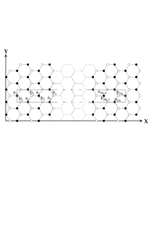
Figure 1: The primitive unit cell of a monolayer graphite in a perpendicular uniform magnetic field.

$\gamma_{0}$(=2.56 eV[2]) is the atom-atom interaction between two neighboring atoms at $\mathbf{R}_{i}$ and $\mathbf{R}_{j}$, and ${|a_{i\mathbf{k}}\rangle}$ ($|b_{j\mathbf{k}}\rangle$) is the linear superposition of the $2p_{z}$ orbitals of the periodic $a_{i}$ ($b_{j}$) atoms [Fig. 1]. The transfer integrals due to three nearest-neighbor atom-atom interactions are given by $t_{1\mathbf{k}}(n)=\gamma_{0}\exp[\,(ik_{x}b^{\prime}/2+ik_{y}\sqrt{3}b^{\prime}/2)+G_{n}\,]$, $t_{2\mathbf{k}}(n)=\gamma_{0}\exp[\,(ik_{x}b^{\prime}/2-ik_{y}\sqrt{3}b^{\prime}/2)-G_{n}\,]$, and $t_{3\mathbf{k}}=\gamma_{0}\exp(\,-ik_{x}b^{\prime}\,)$. $G_{n}=i\pi\Phi[\,(n-1)+1/6\,]$. The magnetic flux would result in the periodical boundary condition along $\hat{x}$ so that the Peierl’s phases are periodic in a period $2/\Phi$(=$2R_{B}$). The rectangular primitive unit cell includes $4R_{B}$ atoms. These atoms define the basis of the Hilbert space and can be used to represent the Hamiltonian matrix. The order of the base functions is very important here. If we naively arrange the base functions in an order as a atomic label [Fig. 1], it would be very difficult in diagonalizing a huge matrix[6]. The dimensionality is $4R_{B}>6400$ for $B<50$ T. To simplify the calculation problem, it is convenient to choose the base functions in the following sequence, $\{|a_{1\mathbf{k}}\rangle,|b_{2R_{B}\mathbf{k}}\rangle,|b_{1\mathbf{k}}\rangle,|a_{2R_{B}\mathbf{k}}\rangle,\ldots|a_{R_{B}\mathbf{k}}\rangle,|b_{R_{B}+1\mathbf{k}}\rangle,|b_{R_{B}\mathbf{k}}\rangle,|a_{R_{B}+1\mathbf{k}}\rangle\}$. The Hamiltonian is then represented as a $4R_{B}\times 4R_{B}$ Hermitian matrix,

$$\left(\begin{array}[]{cccccccc}0&q^{\ast}&p^{\ast}_{1}&0&\ldots&\ldots&0&0\\ q&0&0&p_{2R_{B}}&0&\ldots&\ldots&0\\ p_{1}&0&0&0&q^{\ast}&0&\ldots&0\\ 0&p^{\ast}_{2R_{B}}&0&0&0&q&0&0\\ \vdots&\ddots&q&0&0&\ddots&\ddots&0\\ \vdots&\ldots&\ddots&q^{\ast}&\ddots&\ddots&0&p_{R_{B}+1}\\ 0&\vdots&\vdots&\ddots&\ddots&0&\ddots&q\\ 0&0&0&0&0&p^{\ast}_{R_{B}+1}&q^{\ast}&0\\ \end{array}\right),$$ (10)

where $p_{n}\equiv t_{1\mathbf{k}}(n)+t_{2\mathbf{k}}(n)$ and $q\equiv t_{3\mathbf{k}}$. The range of $k_{x}$ is much smaller than that of $k_{y}$ for $B<50$ T; it is sufficient to focus on energy dispersions along $\hat{k_{y}}$. The unoccupied conduction band ($E^{c}$) is symmetric to the occupied valence band ($E^{\nu}$) at $E_{F}=0$. Only the former is discussed in this work.

The $\pi$-electronic structure at $B=0$ exhibits two kinds of energy dispersions and state degeneracies, as shown in Fig. 2(a). Two nondegenerate linear bands just interact at $E_{F}=0$ or $k_{y}=2\pi/3b^{\prime}$. Other bands are parabolic and doubly degenerate. Figures 2(b)-2(d) at $B=40$ T show that the magnetic field could make electronic states condense and produce Landau levels. The number of magnetic subbands is inversely proportional to $B$. Most of magnetic subbands are flat Landau levels except some oscillatory Landau levels with very weak energy dispersions at $E^{c}\sim\gamma_{0}$ [Fig. 2(c)]. Roughly speaking, a monolayer graphite in the magnetic field could be regarded as a zero-dimensional system. Each discrete Landau level could be expressed as $E^{c}(n)$, where $n=0,1,2,\cdots$ is quantum number. In addition to energy dispersion, the magnetic field also leads to drastic changes in state degeneracy and level spacing. The Landau levels with $E^{c}(n)<\gamma_{0}$ are fourfold degenerate , while others are doubly degenerate. The level spacing ($E_{s}$) between adjacent Landau levels is not equally spaced. $E_{s}$ is maximal between the first two neighboring Landau levels, $E^{c}(0)$ and $E^{c}(1)$ [Fig. 2(b)]. It decreases sharply with n increasing and approaches to zero at $E^{c}\sim\gamma_{0}$ [Fig. 2(c)]. Then it grows gradually in the further increase of n [Fig. 2(d)]. Both state degeneracy and level spacing strongly depend on state energy; therefore, a monolayer graphite is in sharp contrast to a 2D electron gas [16].

The dependence of the Landau-level energies on n and B is quite different from each other at low and high energies. The low Landau levels with $E^{c}(n)\lesssim{}0.4\gamma_{0}$, as shown in Figs. 3(a) and 3(b), are proportional to $\sqrt{n}$ and $\sqrt{B}$ simultaneously. However, there is no simple relation for the high Landau levels with $E^{c}(n)\gtrsim{}0.4\gamma_{0}$. The previous study by the effective-mass approximation predicts the simple relation $E^{c}(n)\propto\sqrt{nB}$ at low energies. Also notice that this method could not account for the complicated relation between $E^{c}$ and ($n,B$) at high energies, and the important differences in state degeneracy and level spacing at different energy regimes.

Density of states, which directly reflects the main characteristics of Landau levels, is

$$D(\omega)=\sum_{\sigma,h=c,\nu}\int_{1stBZ}\frac{dk_{y}}{2\pi}\frac{\Gamma}{\pi}\frac{1}{[\omega-E^{h}(k_{y})]^{2}+\Gamma^{2}},$$ (11)

where the broadening factor is $\Gamma=10^{-3}\gamma_{0}$. $D(\omega)$ without B, as shown by the dashed curve in Figs. 4(a)-4(c), exhibits a vanishing value at $E_{F}=0$, the linear $\omega$-dependence at low frequency, and one symmetric logarithmic divergence at $\omega=\gamma_{0}$. These features are drastically changed by the magnetic field. $D(\omega)$ is finite at $E_{F}=0$ and exhibits a lot of delta-function-like peaks at $\omega\neq 0$. Such prominent peaks come from the 0D Landau levels. The peak height represents the Landau-level degeneracy, so peaks at $\omega<\gamma_{0}$ [Fig. 4(a)] are higher than those at $\omega>\gamma_{0}$ [Fig. 4(c)]. The distribution of peaks is nonuniform because of the unequally spaced Landau levels. The Landau levels with $E^{c}(n)\sim\gamma_{0}$ are oscillatory and dense so that the prominent peaks might be replaced by the weak broadening peaks [Fig. 4(b)]. Density of states is closely related to the available channels of optical excitations. The predicted features could be examined by the optical spectroscopy.

In conclusion, the magneto-electronic properties are calculated by the Peierl’s tight-binding model with the band Hamiltonian matrix. The magnetic field could make linear and parabolic bands become Landau levels. Most of Landau levels are dispersionless, with some oscillatory Landau levels at $E^{c}\sim\gamma_{0}$ excepted. State degeneracy is, respectively, double and fourfold for $E^{c}(n)>\gamma_{0}$ and $E^{c}(n)<\gamma_{0}$. The Landau-level spacing decreases sharply at low energies, while it increases slowly at high energies. The Landau-level energies are characterized by a simple relation $E^{c}(n)\propto\sqrt{nB}$ only for $E^{c}(n)\lesssim 0.4\gamma_{0}$, not for others. Density of states exhibits many delta-function-like prominent peaks, mainly owing to the 0D Landau levels. The effective-mass method can not account for energy dispersion, state degeneracy, level spacing, and dependence of state energy on ($n,B$). The magneto-optical absorption spectra could be used to verify the predicted electronic properties.

This work was supported by the National Science Council of Taiwan, under the Grant Nos. NSC 95-2112-M-006-002.

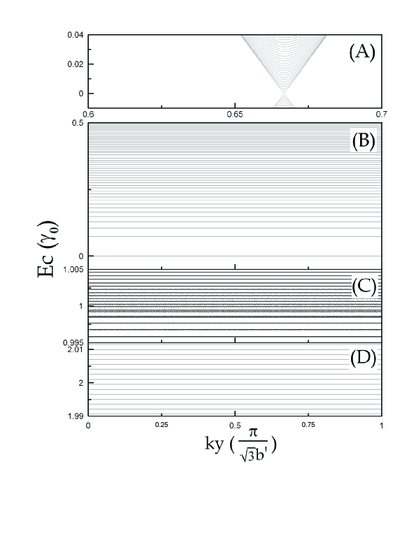
Figure 2: Landau levels of B=40 T at different energy regimes (b), (c), and (d). The low energy bands of B=0 are shown in (a).

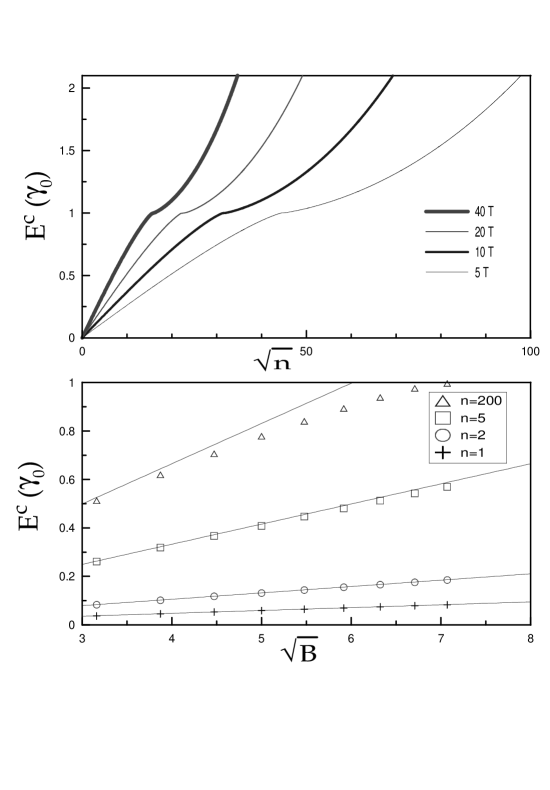
Figure 3: The variation of low Landau-level energies with square root of (a)quantum number and (b)magnetic field. The solid curves in (b) are the linear guidelines.

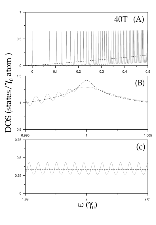
Figure 4: Density of states of B=40 T in different energy regimes (a), (b), and (c). That at B=0 is also shown by the dashed curve.

References

- [1] Wallace P R 1947 Phys. Rev. 71 622
- [2] McClure J W 1956 Phys. Rev. 104 666
- [3] Novoselov K S, Geim A K, Morozov S V, Jiang D, Zhang Y, Dubonos S V, Grigorieva I V and Firsov A A 2004 Science 306 666
- [4] Berger C, Song Z, Li T, Li X, Ogbazghi A Y, Feng R, Dai Z, Marchenkov A N, Conrad E H, First P N and de Heer W A 2004 J. Phys. Chem. B 108 19912
- [5] Novoselov K S, Jiang D, Schedin F, Booth T J, Khotkevich V V, Morozov S V and Geim A K 2005 PNAS 102 10451
- [6] Chang C P, Lu C L, Shyu F L, Chen R B, Fang Y K.and Lin M F 2004 Carbon 42 2975
- [7] Guinea F, Castro Neto A H and Peres N M R 2006 Phys. Rev. B 73 245426
- [8] Shyu F L and Lin M F 2000 J. Phys. Soc. Jpn. 69 607
- [9] Ho J H, Chang C P and Lin M F 2006 Phys. Lett. A 352 446
- [10] Sadowski M L, Martinez G, Potemski M, Berger C and de Heer W A 2006 Phy. Rev. Lett 97 266405
- [11] Ferrari A C, Meyer J C, Scardaci V, Casiraghi C, Lazzeri M, Mauri F, Piscanec S, Jiang D, Novoselov K S, Roth S and Geim A K 2006 Phys. Rev. Lett. 97 187404
- [12] Novoselov K S, McCann E, Morozov S V, Fal’ko V I, Katsnelson M I, Zeitler U, Jiang D, Schedin F and Geim A K 2006 Nature Physics 2 177
- [13] Zhang Y, Tan Y W, Stormer H L and Kim P 2005 Nature 438 201
- [14] Ho J H, Lai Y H, Tsai S J, Hwang J S, Chang C P and Lin M F 2006 J. Phys. Soc. Jpn. 75 114703
- [15] Ho J H, Lai Y H, Lu C L, Hwang J S, Chang C P and Lin M F 2006 Phys. Lett. A 359 70
- [16] Kittel C 1996 Introduction to Solid State Physics, 7th Ed., Wiley