A discrete time neural network model with spiking neurons

Abstract

We derive rigorous results describing the asymptotic dynamics of a discrete time model of spiking neurons introduced in BMS . Using symbolic dynamic techniques we show how the dynamics of membrane potential has a one to one correspondence with sequences of spikes patterns (“raster plots”). Moreover, though the dynamics is generically periodic, it has a weak form of initial conditions sensitivity due to the presence of a sharp threshold in the model definition. As a consequence, the model exhibits a dynamical regime indistinguishable from chaos in numerical experiments.

The description of neuron dynamics can use two distinct representations. On the one hand, the membrane potential is the physical variable describing the state of the neuron and its evolution is ruled by fundamental laws of physics. On the other hand, a neuron is an excitable medium and its activity is manifested by emission of action potential or “spikes”: individual spikes, bursts, spikes trains etc… The first representation constitutes the basis of almost all neuron models, and the Hodgkin-Huxley equations are, from this point of view, certainly one of the most achieved mathematical representation of the neuron HH . However, neurons communicate by emission of spikes, and it is likely that the information is encoded in the neural code, that is, the sequences of spikes exchanged by the neurons and their firing times. Since the spikes emission results from the dynamics of membrane potentials, the information contained in spikes trains is certainly also contained in membrane potential dynamics. But switching from membrane potentials to spikes dynamics allows one to focus on information processing aspects Gerstner . However, this change of description is far from being evident, even when using simple neuron models (see MB for a review). Modeling a spike by a certain shape (Dirac peaks or more complex forms), with a certain refractory period, etc .. which information have we captured and what have we lost ? These questions are certainly too complex to be answered in a general setting (for a remarkable description of spikes dynamics and coding see Spikes ).

Instead, it can be useful to focus on simplified models of neural networks, where the correspondence between the membrane potential dynamics and spiking sequences can be written explicitly. This is one of the goals of the present work. We consider a simple model of spiking neuron, derived from the leaky integrate and fire model Gerstner , but where the time is discretised. To be the best of our knowledge, this model has been first introduced by G. Beslon, O. Mazet and H. Soula HS ,BMS , and we shall call it “the BMS model”. Certainly, the simplifications involved, especially the time discretisation, raise delicate problems concerning biological interpretations, compared to more elaborated models or to biological neurons CV (see the discussion section). But the main interest of the model is its simplicity and the fact that, as shown in the present paper, one can establish an explicit one-to-one correspondence between the membrane potential dynamics and the dynamics of spikes. Thus, no information is lost when switching from one description to the other, even when the spiking sequences have a complex structure. Moreover, this correspondence opens up the possibility of using tools from dynamical systems theory, ergodic theory, and statistical physics to address questions such as:

• How to measure the information content of a spiking sequence ?

• What is the effect of synaptic plasticity (Long Term Depression, Long Term Potentiation, Spike Time Dependent Plasticity, Hebbian learning) on the spiking sequences displayed by the neural network ?

• What is the relation between a presented input and the resulting spiking sequence, before and after learning.

• What is the effect of stochastic perturbations ? Can we relate the dynamics of the discrete time BMS model with noise to previous studies on continuous time Integrate and Fire neural networks perturbed by a Brownian noise (e.g. BrunHak ,RBH ) ?

This paper is the first one of a series trying to address some of these questions in the context of BMS model. The goal the present article, is to pose the mathematical framework used for subsequent developments. In section 2 we present the BMS model and provide elementary mathematical results on the system dynamics. We show that the presence of a sharp threshold for the model definition of neuron firing induces singularities responsible for a weak form of initial conditions sensitivity. This effect is different from the usual notion of chaos since it arises punctually, whenever a trajectory intersects a zero Lebesgue measure set, called the singularity set. Similar effects are encountered in billiards Chernov or in Self-Organized Criticality BCK1 ,BCK2 ,BCKM . Applying methods from dynamical systems theory we derive rigorous results describing the asymptotic dynamics in section 3. Although we show that the dynamics is generically periodic, the presence of a singularity set has strong effects. In particular the number of periodic orbits and the transients growth exponentially as the distance between the attractor and the singularity set tends to zero. This has a strong impact on the numerics and there is a dynamical regime numerically indistinguishable from chaos. Moreover, these effects become prominent when perturbing the dynamics or when the infinite size limit is considered. In this context we discuss the existence of a Markov partition allowing to encode symbolically the dynamics with “spike trains”. In section 4 we indeed show that there is a one to one correspondence between the membrane potential dynamics and the sequences of spiking patterns (“raster plots”). This opens up the possibility to use methods from ergodic theory and statistical mechanics (thermodynamic formalism) to analyse spiking sequences. This aspect will be the central topic of another paper. As an example, we briefly analyze the case of random synapses and inputs on the dynamics and compare our analysis to the results obtained by BMS in BMS ,HS . We exhibit numerically a sharp transition between a neural death regime where all neurons are asymptotically silent, and a phase with long transient having the appearance of a chaotic dynamics. This transition occurs for example when the variance of the synaptic weights increases. A further increase leads to a periodic dynamics with small period. In the discussion section we briefly comment some extensions (effect of Brownian noise, use of Gibbs measure to characterize the statistics of spikes) that will be developed in forthcoming papers.

Warning This paper is essentially mathematically oriented (as the title suggests), although some extensive parts are devoted to the interpretation and consequences of mathematical results for neural networks. Though the proof of theorems and the technical parts can be skipped, the non mathematician reader interested in computational neurosciences, may nevertheless have difficulties to find what he gains from this study. Let us briefly comment this point. There is still a huge distance between the complexity of the numerous models of neurons or neural networks, and the mathematical analysis of their dynamics, though a couple of remarkable results have been obtained within the 50 past years (see e.g. CS and references therein). This has several consequences and drawbacks. There is a constant temptation to simplify again and again the canonical equations for the neuron dynamics (e.g. Hodgkin-Huxley equations) to obtain apparently tractable models. A typical example concerns integrate and fire (IF) models. The introduction of sharp threshold and instantaneous reset gives a rather simple formulation of neuron activity, and, at the level of an isolated neuron, a couple of important quantities such as the next time of firing can be computed exactly. The IF structure can be extended to conductance based models RD ; CV closer to biological neurons. However, there are quite a few rigorous results dealing with the dynamics of IF models at the network level. The present paper provides an example of an IF Neural Network analysed in a global and rigorous manner.

The lack of mathematical results concerning the dynamics of neural networks has other consequences. There is an extensive use of numerical simulations, which is fine. But the present paper shows the limits of numerics in a model where “neurons” have a rather simple structure. What is for more elaborated models ? It also warns the reader against the uncontrolled use of terminologies such as “chaos, edge of chaos, complexity”. In this paper, mathematics allows us to precisely define and analyse mechanisms generating initial conditions sensitivity, which are basically presents in all IF neural networks, since they are due to the sharp threshold. We also give a precise meaning to the “edge of chaos” and actually give a way to locate it. We evidence mechanisms, such as the first firing of a neuron after an arbitrary large time, which can basically exist in real neural networks, and raise huge difficulties when willing to decide, experimentally or numerically, what is the nature of dynamics. Again, what happens for more elaborated models ? This work is a first step in providing a mathematical setting allowing to handle these questions for more elaborated IF neural networks models CV .

1 General context.

1.1 Model definition.

Fix $N>0$ a positive integer called “the dimension of the neural network” (the number of neurons). Let ${\cal W}$ be an $N\times N$ matrix, called “the matrix of synaptic weights”, with entries $W_{ij}$. It defines an oriented and signed graph, called “the neural network associated to ${\cal W}$”, with vertices $i=1\dots N$ called the “neurons”. There is oriented edge $j\to i$ whenever $W_{ij}\neq 0$. $W_{ij}$ is called “the synaptic weight from neuron $j$ to neuron $i$”. The synaptic weight is called “excitatory” if $W_{ij}>0$ and “inhibitory” if $W_{ij}<0$.

Each vertex (neuron) $i$ is characterized by a real variable $V_{i}$ called the “membrane potential of neuron $i$”. Fix a positive real number $\theta>0$ called the “firing threshold”. Let $Z$ be the function $Z(x)=\chi(x\geq\theta)$ where $\chi$ is the indicatrix function. Namely, $Z(x)=1$ whenever $x\geq\theta$ and $Z(x)=0$ otherwise. $Z(V_{i})$ is called the “firing state of neuron $i$”. When $Z(V_{i})=1$ one says that neuron $i$ “fires” and when $Z(V_{i})=0$ neuron $i$ is “quiescent”. Finally, fix $\gamma\in[0,1[$, called the “leak rate”. The discrete time and synchronous dynamics of the BMS model is given by:

$${\bf V}(t+1)={\bf F}({\bf V}(t)),$$ (1)

where ${\bf V}=\left\{V_{i}\right\}_{i=1}^{N}$ is the vector of membrane potentials and ${\bf F}=\left\{F_{i}\right\}$ with:

$$F_{i}({\bf V})=\gamma V_{i}\left(1-Z[V_{i}]\right)+\sum_{j=1}^{N}W_{ij}Z[V_{j}]+I^{ext}_{i};\qquad i=1\dots N.$$ (2)

The variable $I^{ext}_{i}$ is called “the external current applied to neuron $i$”. We shall assume in this paper that this current does not depend on time (see however the discussion section from an extension of the present results to time dependent external currents). The dynamical system (1) is then autonomous.

In the following we shall use the quantity

$$I^{s}_{i}({\bf V})=\sum_{j=1}^{N}W_{ij}Z[V_{j}].$$ (3)

called the “synaptic current” received by neuron $i$. The “total current” is :

$$I_{i}({\bf V})=I^{s}_{i}({\bf V})+I^{ext}_{i}$$ (4)

Define the firing times of neuron $i$, for the trajectory ${\bf V}$, by:

$$\tau_{i}^{(k)}({\bf V})=\inf\left\{t\ |t>\tau_{i}^{(k-1)}({\bf V}),\ V_{i}(t)\geq\theta\right\}$$ (5)

where $\tau_{i}^{0}=-\infty$.

1.2 Interpretation of BMS model as a Neural Network.

The BMS model is based on the evolution equation for the leaky integrate and fire neuron Gerstner :

$$\frac{dV_{i}}{dt}=-\frac{V_{i}}{\tau}+\frac{I_{i}(t)}{C}$$ (6)

where $\tau=RC$ is the integration time scale, with $R$, the membrane resistance and $C$ the electric capacitance of the membrane. $I_{i}(t)$ is the synaptic current (spikes emitted by other neurons and transmitted to neuron $i$ via the synapses $j\to i$) and an external current. The equation (6) holds whenever the membrane potential is smaller than a threshold $\theta$, usually depending on time (to account for characteristics such as refractory period of the neuron). When the membrane potential exceeds the threshold value, the neuron “fires” (emission of an action potential or “spike”). The spike shape depends on the model. In the present case, the membrane potential is reset instantaneously to a value $V_{reset}$, corresponding to the value of the membrane potential when the neuron is at rest. More elaborated models can be proposed accounting for refractory period, spikes shapes, etc … Gerstner

A formal time discretization of (6) (say with an Euler scheme) gives:

$$V_{i}(t+dt)=V_{i}(t)\left(1-\frac{dt}{\tau}\right)+\frac{I_{i}(t)}{C}dt$$ (7)

Setting $dt=1$ and $\gamma=1-\frac{1}{\tau}$, we obtain.

$$V_{i}(t+1)=\gamma V_{i}(t)+\frac{I_{i}(t)}{C}$$ (8)

This discretization imposes that $\tau\geq 1$ in (6), thus $\gamma\in[0,1[$. This equation holds whenever $V_{i}(t)<\theta$. As discussed in e.g. Iz it provides a rough but realistic approximation of biological neurons behaviours. Note that in biological neurons, a spike duration is not negligible but has a finite duration (of order $1$ ms).

The firing of neuron $i$ is characterized by:

$$V_{i}(\tau_{i}^{(k)})\geq\theta$$

and:

$$V_{i}(\tau^{(k)}_{i}+1)=V_{reset}+I_{i}(\tau^{(k)})$$ (9)

where, from now on, we shall consider that $C=1$ and that $V_{reset}$, the reset potential, is equal to $0$. Introducing the function $Z$ allows us to write the neuron evolution before and after firing in a unique equation (2). Moreover, this apparently naive token provides useful insights in terms of symbolic dynamics and interpretation of neural coding.

Note that the firing is not instantaneous. The membrane potential is maintained at a value $\theta$ during the time interval $[\tau^{(k)}_{i},\tau^{(k)}_{i}+1[$. Note also that simultaneous firing of several neurons can occur. Moreover, a localized excitation may induce a chain reaction where $n_{1}$ neurons fire at the next time, inducing the firing of $n_{2}$ neurons, etc $\dots$. Thus, a localized input may generate a network reaction on an arbitrary large space scale, in a relatively short time scale. The evolution of this propagation phenomenon depends on the synaptic weights and on the membrane potential values of the nodes involved in the chain reaction. This effect, reminiscent of the “avalanches” observed in the context of self-organized criticality Bak , may have an interesting incidence in the neural network (1).

2 Preliminary results.

2.1 Phase space ${\cal M}$.

Since $\gamma<1$ one can restrict the phase space of (1) to a compact set ${\cal M}=[V_{min},V_{max}]^{N}$ such that ${\bf F}({\cal M})\subset{\cal M}$ where:

$$V_{min}=\min(0,\frac{1}{1-\gamma}\left[\min_{i=1\dots N}\sum_{j|W_{ij}<0}W_{ij}+I^{ext}_{i}\right]),$$ (10)

and:

$$V_{max}=\max(0,\frac{1}{1-\gamma}\left[\max_{i=1\dots N}\sum_{j|W_{ij}>0}W_{ij}+I^{ext}_{i}\right]),$$ (11)

where we use the convention $\sum_{j\in\emptyset}W_{ij}=0$. Therefore, $\sum_{j|W_{ij}<0}W_{ij}=0$ (resp. $\sum_{j|W_{ij}>0}W_{ij}=0$) if all weights are positive (resp. negative) and $\sum_{j|W_{ij}<0}W_{ij}\leq 0$ (resp. $\sum_{j|W_{ij}>0}W_{ij}\geq 0)$.

This results is easy to show. Indeed, assume that for all neurons, $V_{min}\leq V_{i}\leq V_{max}$. Then, the membrane potential of neuron $i$ at the next iteration is

$$V^{\prime}_{i}=\gamma V_{i}(1-Z(V_{i}))+\sum_{j}W_{ij}Z(V_{j})+I^{ext}_{i}.$$

Therefore,

$$\gamma V_{min}(1-Z(V_{i}))+\sum_{j|W_{ij}<0}W_{ij}+I^{ext}_{i}\leq V^{\prime}_{i}\leq\gamma V_{max}(1-Z(V_{i}))+\sum_{j|W_{ij}>0}W_{ij}+I^{ext}_{i}.$$

If $V_{min}<0$ then,

$$V_{min}=\gamma V_{min}+\displaystyle{\min_{i=1\dots N}}\left[\sum_{j|W_{ij}<0}W_{ij}+I^{ext}_{i}\right]\leq\gamma V_{min}(1-Z(V_{i}))+\sum_{j|W_{ij}<0}W_{ij}+I^{ext}_{i}\leq V^{\prime}_{i},$$

and if $V_{min}=0$, then necessarily $\displaystyle{\min_{i=1\dots N}}\left[\sum_{j|W_{ij}<0}W_{ij}+I^{ext}_{i}\right]\geq 0$ and $V^{\prime}_{i}\geq 0=V_{min}$.

Similarly, if $V_{max}>0$ then,

$$\gamma V_{max}(1-Z(V_{i}))+\sum_{j|W_{ij}>0}W_{ij}+I^{ext}_{i}\leq\gamma V_{max}+\displaystyle{\max_{i=1\dots N}}\left[\sum_{j|W_{ij}>0}W_{ij}+I^{ext}_{i}\right]=V_{max}.$$

and if $V_{max}=0$, then necessarily $\displaystyle{\max_{i=1\dots N}}\left[\sum_{j|W_{ij}>0}W_{ij}+I^{ext}_{i}\right]\leq 0$ and $V^{\prime}_{i}\leq 0=V_{max}$.

Note that the similar bounds hold if $I^{ext}_{i}$ depends on time.

2.2 Phase space ${\cal M}$.

For each neuron one can decompose the interval ${\cal I}=[V_{min},V_{max}]$ into ${\cal I}_{0}\cup{\cal I}_{1}$ with ${\cal I}_{0}=[V_{min},\ \theta[$, ${\cal I}_{1}=[\theta,V_{max}]$. If $V\in{\cal I}_{0}$ the neuron is quiescent, otherwise it fires. This splitting induces a partition ${\cal P}$ of ${\cal M}$, that we call the “natural partition”. The elements of ${\cal P}$ have the following form. Call $\Lambda=\left\{0,1\right\}^{N}$. Let $\mbox{{\boldmath$\eta$}}=\left\{\eta_{1},\dots,\eta_{N}\right\}\in\Lambda$. This is a $N$ dimensional vector with binary components $0,1$. We call such a vector a spiking state. Then ${\cal M}=\displaystyle{\bigcup_{\mbox{{\boldmath$\eta$}}\in\Lambda}{{\cal M}_{\mbox{{\boldmath$\eta$}}}}}$ where:

$${{\cal M}_{\mbox{{\boldmath$\eta$}}}}=\left\{{\bf V}\in{\cal M}\ |\ V_{i}\in{\cal I}_{\eta_{i}}\right\}$$ (12)

Equivalently, ${\bf V}\in{{\cal M}_{\mbox{{\boldmath$\eta$}}}}\Leftrightarrow Z(V_{i})=\eta_{i},\ i=1\dots N$. Therefore, the partition ${\cal P}$ corresponds to classifying the membrane potential vectors according to their spiking state. More precisely, call:

$${\cal D}(\mbox{{\boldmath$\eta$}})=\left\{i\in\left\{1\dots N\right\}\ |\ \eta_{i}=1\right\},$$ (13)

and $\bar{{\cal D}}(\mbox{{\boldmath$\eta$}})$ the complementary set $\left\{i\in\left\{1\dots N\right\}\ |\ \eta_{i}=0\right\}$. Then, whatever the membrane potential ${\bf V}\in{{\cal M}_{\mbox{{\boldmath$\eta$}}}}$ the neurons whose index $i\in{\cal D}(\mbox{{\boldmath$\eta$}})$ will fire at the next iteration while the neurons whose index $i\in\bar{{\cal D}}(\mbox{{\boldmath$\eta$}})$ will stay quiescent. In particular, the synaptic current (3) is fixed by the domain ${{\cal M}_{\mbox{{\boldmath$\eta$}}}}$ since :

$$I^{s}_{i}({\bf V})\equiv I^{s}_{i}(\mbox{{\boldmath$\eta$}})=\sum_{j\in{\cal D}(\mbox{{\boldmath$\eta$}})}W_{ij}$$ (14)

whenever ${\bf V}\in{{\cal M}_{\mbox{{\boldmath$\eta$}}}}$. In the same way we shall write $I_{i}(\mbox{{\boldmath$\eta$}})=I^{s}_{i}(\mbox{{\boldmath$\eta$}})+I^{ext}_{i}$.

${\cal P}$ has a simple product structure. Its domains are hypercubes (thus they are convex) where the edges are parallels to the directions ${\bf e}_{i}$ (basis vectors of ${\sf I\!R}^{N}$). More precisely, for each $\mbox{{\boldmath$\eta$}}\in\left\{0,1\right\}^{N}$,

$${{\cal M}_{\mbox{{\boldmath$\eta$}}}}=\prod_{i=1}^{N}I_{\eta_{i}},$$ (15)

where $\prod$ denotes the Cartesian product.

2.3 Elementary properties of ${\bf F}$.

Some elementary, but essential properties of ${\bf F}$, are summarized in the following proposition. We use the notation

$${\cal C}(\mbox{{\boldmath$\eta$}})=\sum_{j=1}^{N}\eta_{j}=\#{\cal D}(\mbox{{\boldmath$\eta$}}),$$ (16)

for the cardinality of ${\cal D}(\mbox{{\boldmath$\eta$}})$. This is the number of neurons that will fire in the next iteration whenever the spiking pattern is $\eta$.

Proposition 1

Denote by ${\bf F}_{\mbox{{\boldmath$\eta$}}}$ the restriction of ${\bf F}$ to the domain ${{\cal M}_{\mbox{{\boldmath$\eta$}}}}$. Then whatever $\mbox{{\boldmath$\eta$}}\in\Lambda$,

1. ${\bf F}_{\mbox{{\boldmath$\eta$}}}$ is affine and differentiable in the interior of its domain ${{\cal M}_{\mbox{{\boldmath$\eta$}}}}$.

2. ${\bf F}_{\mbox{{\boldmath$\eta$}}}$ is a a contraction with coefficient $\gamma(1-\eta_{i})$ in direction $i$.

3. Denote by $D{\bf F}_{\mbox{{\boldmath$\eta$}}}$ the Jacobian matrix of ${\bf F}_{\mbox{{\boldmath$\eta$}}}$. Then $D{\bf F}_{\mbox{{\boldmath$\eta$}}}$ has ${\cal C}(\mbox{{\boldmath$\eta$}})$ zero eigenvalues and $N-{\cal C}(\mbox{{\boldmath$\eta$}})$ eigenvalues $\gamma$.

4. Call $F_{\mbox{{\boldmath$\eta$}},i}$ the $i$-th component of ${\bf F}_{\mbox{{\boldmath$\eta$}}}$ then

   $${\bf F}({{\cal M}_{\mbox{{\boldmath$\eta$}}}})={\bf F}_{\mbox{{\boldmath$\eta$}}}\left[\prod_{i=1}^{N}{\cal I}_{\eta_{i}}\right]=\prod_{i=1}^{N}F_{\mbox{{\boldmath$\eta$}},i}({\cal I}_{\eta_{i}})$$ (17)

   where $F_{\mbox{{\boldmath$\eta$}},i}({\cal I}_{0})$ is the interval $[\gamma V_{min}+\sum_{j=1}^{N}W_{ij}\eta_{j}+I^{ext}_{i},\gamma\theta+\sum_{j=1}^{N}W_{ij}\eta_{j}+I^{ext}_{i}[$ and $F_{\mbox{{\boldmath$\eta$}},i}({\cal I}_{1})$ is the point $\sum_{j=1}^{N}W_{ij}\eta_{j}+I^{ext}_{i}$. More precisely, if ${\cal C}(\mbox{{\boldmath$\eta$}})=k$, the image of ${{\cal M}_{\mbox{{\boldmath$\eta$}}}}$ is a $N-k$ dimensional hypercube, with faces parallel to the canonical basis vectors ${\bf e}_{i}$ for all $i\notin D(\mbox{{\boldmath$\eta$}})$ and with a volume $\gamma^{N-k}\left[\theta-V_{min}\right]^{N-k}$.

According to item (1) we call the domains ${{\cal M}_{\mbox{{\boldmath$\eta$}}}}$, “domains of continuity”of ${\bf F}$.

Proof

By definition, $\forall{\bf V}\in{{\cal M}_{\mbox{{\boldmath$\eta$}}}}$, ${\bf F}_{i}({\bf V})=\gamma V_{i}(1-\eta_{i})+\sum_{j=1}^{N}W_{ij}\eta_{j}+I^{ext}_{i}$. ${\bf F}$ is therefore piecewise affine, with a constant $I_{i}(\mbox{{\boldmath$\eta$}})=\sum_{j\in{\cal D}(\mbox{{\boldmath$\eta$}})}W_{ij}+I^{ext}_{i}$ fixed by the domain ${{\cal M}_{\mbox{{\boldmath$\eta$}}}}$. Moreover ${\bf F}_{\mbox{{\boldmath$\eta$}}}$ is differentiable on the interior of each domain ${{\cal M}_{\mbox{{\boldmath$\eta$}}}}$, with:

$$\frac{\partial F_{\mbox{{\boldmath$\eta$}},i}}{\partial V_{j}}=\gamma\delta_{ij}[1-\eta_{i}].$$ (18)

The corresponding Jacobian matrix is thus diagonal, constant in the domain ${{\cal M}_{\mbox{{\boldmath$\eta$}}}}$, and its eigenvalues are $\gamma[1-\eta_{i}]$. Each eigenvalue is therefore $0$ if $\eta_{i}=1$ (neuron $i$ fires) and $\gamma$ if $\eta_{i}=0$ (neuron $i$ is quiescent). Thus, since $\gamma<1$, ${\bf F}_{\mbox{{\boldmath$\eta$}}}$ is a contraction in each direction $i$. Once ${{\cal M}_{\mbox{{\boldmath$\eta$}}}}$ has been fixed, the image of each coordinate $V_{i}$ is only a function of $V_{i}$. Thus, if $V\in{{\cal M}_{\mbox{{\boldmath$\eta$}}}}=\prod_{i=1}^{N}{\cal I}_{\eta_{i}}$, then $F_{\mbox{{\boldmath$\eta$}},i}({\bf V})=F_{\mbox{{\boldmath$\eta$}},i}(V_{i})$ and ${\bf F}_{\mbox{{\boldmath$\eta$}}}$ maps the hypercube ${{\cal M}_{\mbox{{\boldmath$\eta$}}}}=\prod_{i=1}^{N}{\cal I}_{\eta_{i}}$ onto the hypercube $\prod_{i=1}^{N}F_{\mbox{{\boldmath$\eta$}},i}({\cal I}_{\eta_{i}})$. The segments ${\cal I}_{\eta_{i}}$ with $\eta_{i}=0$ are mapped to parallel segments $[\gamma V_{min}+\sum_{j=1}^{N}W_{ij}\eta_{j}+I^{ext}_{i},\gamma\theta+\sum_{j=1}^{N}W_{ij}\eta_{j}+I^{ext}_{i}[$ while each segment ${\cal I}_{\eta_{i}}$ with $\eta_{i}=1$ is mapped to a point. Thus, if ${\cal C}(\mbox{{\boldmath$\eta$}})=k$ the image of ${{\cal M}_{\mbox{{\boldmath$\eta$}}}}$ is a $N-k$ dimensional hypercube, with faces parallel to the canonical basis vectors ${\bf e}_{i}$, where $i\notin D(\mbox{{\boldmath$\eta$}})$ and with a volume $\gamma^{N-k}\left[\theta-V_{min}\right]^{N-k}$. ∎

Finally, we note the following property. The dynamical system (1) can be defined on ${\sf I\!R}^{N}$ and the contraction property extends to this space. If one considers the $\delta$-ball ${\cal B}_{\cal M}(\delta)=\left\{{\bf V}\in{\sf I\!R}^{N}|d({\bf V},{\cal M})<\delta\right\}$ then :

$${\bf F}\left[{\cal B}_{\cal M}(\delta)\right]\subset{\cal B}_{\cal M}(\delta).$$ (19)

The distance $d$ is, for example :

$$d({\bf X},{\bf X}^{\prime})=\max_{i=1\dots N}|X_{i}-X^{\prime}_{i}|,$$ (20)

natural in the present context according to property 1 (eq. (17)).

2.4 The singularity set ${\cal S}$.

The set

$${\cal S}=\left\{{\bf V}\in{\cal M},\ |\exists i,\ V_{i}=\theta\right\},$$ (21)

is called the singularity set for the map ${\bf F}$. ${\bf F}$ is discontinuous on ${\cal S}$. This set has a simple structure: this is a finite union of $N-1$ dimensional hyperplanes corresponding to faces of the hypercubes ${{\cal M}_{\mbox{{\boldmath$\eta$}}}}$. Though ${\cal S}$ is a “small” set both from the topological (non residual set) and metric (zero Lebesgue measure) point of view, it has an important effect on the dynamics.

Indeed, let us consider the trajectory of a point ${\bf V}\in{\cal M}$ and perturbations with an amplitude $<\epsilon$ about ${\bf V}$. Equivalently, consider the evolution of the $\epsilon$ ball ${\cal B}({\bf V},\epsilon)$ under ${\bf F}$. If ${\cal B}({\bf V},\epsilon)\cap{\cal S}=\emptyset$ then by definition ${\cal B}({\bf V},\epsilon)\subset\stackrel{{\scriptstyle\circ}}{{{{\cal M}_{\mbox{{\boldmath$\eta$}}}}}}$, some $\eta$, where $\stackrel{{\scriptstyle\circ}}{{{{\cal M}_{\mbox{{\boldmath$\eta$}}}}}}$ is the interior of the domain ${{\cal M}_{\mbox{{\boldmath$\eta$}}}}$. Thus, by prop. 1(2) ${\bf F}[{\cal B}({\bf V},\epsilon)]\subset{\cal B}({\bf F}({\bf V}),\gamma\epsilon)$. More generally, if the images of ${\cal B}({\bf V},\epsilon)$ under ${\bf F}^{t}$ never intersect ${\cal S}$, then, at time $t$, ${\bf F}^{t}[{\cal B}({\bf V},\epsilon)]\subset{\cal B}({\bf F}^{t}({\bf V}),\gamma^{t}\epsilon)$. Since $\gamma<1$, there is a contraction of the initial ball, and the perturbed trajectories about ${\bf V}$ become asymptotically indistinguishable from the trajectory of ${\bf V}$. (Actually, if all neurons have fired after a finite time $t$ then all perturbed trajectories collapse onto the trajectory of ${\bf V}$ after $t+1$ iterations).

On the opposite, assume that there is a time, $t_{0}$ such that ${\bf F}^{t_{0}}({\cal B}({\bf V},\epsilon))\cap{\cal S}\neq\emptyset$. By definition, this means that there exists a subset of neurons $\left\{i_{1},\dots,i_{k}\right\}$ and ${\bf V}^{\prime}\in{\cal B}({\bf V},\epsilon)$, such that $Z(V_{i}(t_{0}))\neq Z(V^{\prime}_{i}(t_{0}))$, $i\in\left\{i_{1},\dots,i_{k}\right\}$. Then:

$$\begin{array}[]{lr}F_{i}({\bf V}(t_{0}))-F_{i}({\bf V}^{\prime}(t_{0}))=&\\ \gamma\left[V_{i}(t_{0})(1-Z(V_{i}(t_{0})))-V^{\prime}_{i}(t_{0})(1-Z(V^{\prime}_{i}(t_{0})))\right]+\sum_{j\in\left\{i_{1},\dots,i_{k}\right\}}W_{ij}\left[Z(V_{j}(t_{0}))-Z(V^{\prime}_{j}(t_{0}))\right]&\end{array}$$

In this case, the difference between $F_{i}({\bf V}(t_{0}))-F_{i}({\bf V}^{\prime}(t_{0}))$ is not proportional to $V_{i}(t_{0})-V^{\prime}_{i}(t_{0})$ , for $i\in\left\{i_{1},\dots,i_{k}\right\}$. Moreover, this distance is finite while $|V_{i}(t_{0})-V^{\prime}_{i}(t_{0})|<\epsilon$ can be arbitrary small. Thus, in this case, the crossing of ${\cal S}$ by the $\epsilon$-ball induces a strong separation effect reminiscent of initial condition sensitivity in chaotic dynamical system. But the main difference with chaos is that the present effect occurs only when the ball crosses the singularity. (Otherwise the ball is contracted). The result is a weak form of initial condition sensitivity and unpredictability occurring also in billiards Chernov or in models of self-organized criticality BCK1 ,BCK2 . Therefore, ${\cal S}$ is the only source of complexity of the BMS model, and its existence is due to the strict threshold in the definition of neuron firing.

Note that if one replaces the sharp threshold by a smooth one (this amounts to replacing an Heaviside function by a sigmoid) then the dynamics become expansive in the region where the slope of the regularized threshold is larger than $1$. Then, the model exhibits chaos in the usual sense (see e.g. PD ,JP ). Thus, in some sense, the present model can be viewed as a limit of a regular neural network with a sigmoidal transfer function. However, when dealing with asymptotic dynamic one has to consider two limits ($t\to+\infty$ and slope $\to+\infty$) that may not commute.

3 Asymptotic dynamics.

We now focus on the asymptotic dynamics of (1).

3.1 The $\omega$-limit set.

Definition 1

(From KH ; GH ) A point $y\in{\cal M}$ is called an $\omega$-limit point for a point $x\in{\cal M}$ if there exists a sequence of times $\left\{t_{k}\right\}_{k=0}^{+\infty}$, such that $x(t_{k})\to y$ as $t_{k}\to+\infty$. The $\omega$-limit set of $x$, $\omega(x)$, is the set of all $\omega$-limit points of $x$. The $\omega$-limit set of ${\cal M}$, denoted by $\Omega$, is the set $\Omega=\bigcup_{x\in{\cal M}}\omega(x)$.

Equivalently, $\Omega$ is the set of accumulation points of ${\bf F}^{t}({\cal M})$. In the present case, since ${\cal M}$ is closed and invariant, we have $\Omega=\bigcap_{t=0}^{\infty}{\bf F}^{t}({\cal M})$.

The notion of $\omega$ limit set is less known and used than the notion of attractor. There are several distinct definition of attractor. For example, according to KH :

Definition 2

A compact set ${\cal A}\in{\cal M}$ is called an attractor for ${\bf F}$ if there exists a neighborhood ${\cal U}$ of ${\cal A}$ and a time $N>0$ such that ${\bf F}^{N}({\cal U})\subset{\cal U}$ and

$${\cal A}=\displaystyle{\bigcap_{t=0}^{\infty}{\bf F}^{t}({\cal U})}.$$ (22)

Note that from equation (19) one may choose for ${\cal U}$ any open set such that:

$${\cal U}\supset{\cal B}_{\cal M}(\delta),\ \forall\delta>0.$$ (23)

In our case ${\cal A}$ and $\Omega$ coincide whenever ${\cal A}$ is not empty. However, there are cases where the attractor is empty while the $\omega$ limit set is not (see example of Fig. 3.3.1 in KH , page 128). We shall actually encounter the same situation in section 3.4. For this reason we shall mainly use the notion of $\omega$-limit set instead of the notion of attractor, though we shall see that they coincide except for a non generic set of synaptic weights and external currents.

3.2 Local stable manifolds.

The stable manifold of ${\bf V}$ is the set:

$${\cal W}^{s}({\bf V})=\left\{{\bf V}^{\prime}\ |d\left({\bf F}^{t}({\bf V}^{\prime}),{\bf F}^{t}({\bf V})\right)\to 0\quad t\to+\infty\right\}.$$ (24)

The local stable manifold ${\cal W}^{s}_{loc}({\bf V})$ is the largest connected component of ${\cal W}^{s}({\bf V})$ containing ${\bf V}$. It obeys:

$${\bf F}\left[{\cal W}^{s}_{loc}({\bf V})\right]\subset{\cal W}^{s}_{loc}({\bf F}({\bf V})).$$ (25)

In the present model, if ${\bf V}$ has a local stable manifold ${\cal W}^{s}_{\epsilon}({\bf V})$ of diameter $\epsilon$ then:

$${\bf F}^{t}\left[{\cal W}^{s}_{\epsilon}({\bf V})\right]\subset{\cal W}^{s}_{\gamma^{t}\epsilon}({\bf F}^{t}({\bf V})).$$ (26)

Thus, a perturbation of amplitude $<\epsilon$ is exponentially damped and the asymptotic dynamics of any point belonging to the local stable manifold of ${\bf V}$ is indistinguishable from the evolution of ${\bf V}$.

In BMS model some point may not have a local stable manifold, due to the presence of the singularity set. Indeed, if a small ball of size $\epsilon$ and center ${\bf V}$ intersects ${\cal S}$ it will be cut into several pieces strongly separated by the dynamics. If this happens, ${\bf V}$ does not have a local stable manifold of size $\epsilon$. According to (26) a point ${\bf V}\in{\cal M}$ has a local stable manifold of diameter $\epsilon$ if :

$${\bf V}\notin\bigcap_{t_{0}\geq 0}\bigcup_{t\geq t_{0}}{\bf F}^{-t}({\cal U}_{\gamma^{t}\epsilon}({\cal S})),$$ (27)

where ${\cal U}_{\delta}({\cal S})=\left\{{\bf V}\ |\ d({\bf V},{\cal S})<\delta\right\}$ is the $\delta$-neighborhood of ${\cal S}$. This means that the dynamics contracts the $\epsilon$ ball faster than it approaches the singularity set. A condition like (27) is useful for measure-theoretic estimations of the set of points having no stable manifold via the Borel-Cantelli lemma.

In the present context, a more direct approach consists in computing:

$$d(\tilde{{\bf V}}^{+},{\cal S})=\inf_{t\geq 0}\min_{i=1\dots N}|V_{i}(t)-\theta|,$$ (28)

which measures the “distance” between the forward trajectory $\tilde{{\bf V}}^{+}\stackrel{{\scriptstyle\rm def}}{{=}}\left\{{\bf V}(t)\right\}_{t\geq 0}$ of ${\bf V}$ and ${\cal S}$. One has the following:

Proposition 2

If $d(\tilde{{\bf V}}^{+},{\cal S})>\epsilon>0$ then ${\bf V}$ has a local stable manifold of diameter $\epsilon$.

Proof

This results directly from proposition 1. Indeed, if $d(\tilde{{\bf V}}^{+},{\cal S})>\epsilon$, the image of the $\epsilon$-ball ${\cal B}({\bf V},\epsilon)$ under ${\bf F}^{t}$, belong to a unique continuity domain of ${\bf F}$, $\forall t>0$ and ${\bf F}$ is contracting on each domain of continuity. ∎

In the same way, one defines the distance of the omega limit set $\Omega$ to the singularity set (one may also consider the distance to the attracting set whenever ${\cal A}$ is not empty):

$$d(\Omega,{\cal S})=\inf_{{\bf V}\in\Omega}d(\tilde{{\bf V}}^{+},{\cal S}).$$ (29)

The distance vanishes if and only if $\Omega\cap{\cal S}\neq\emptyset$. Thus, if $d(\Omega,{\cal S})>\epsilon>0$ any point of $\Omega$ has a local stable manifold. In this situation, any $\epsilon$- perturbation about ${\bf V}\in\Omega$ is asymptotically damped. Note however that $d(\Omega,{\cal S})$ can be positive but arbitrary small (see section 5.1).

3.3 Symbolic coding and Markov partition.

The partition ${\cal P}$ provides a natural way for encoding the dynamics. Indeed, to each forward trajectory $\tilde{{\bf V}}^{+}$ one can associate an infinite sequence of spiking patterns $\mbox{{\boldmath$\eta$}}_{1},\dots,\mbox{{\boldmath$\eta$}}_{t}\dots$ where $\mbox{{\boldmath$\eta$}}_{t}=\left\{\eta_{i;t}=Z(V_{i}(t))\right\}_{i=1}^{N}$. This sequence provides exactly the times of firing for each neuron. It contains thus the “neural code” of the BMS model. In fact, this sequence is exactly what biologists call the “raster plot” Gerstner . On the other hand, knowing the spiking sequence and the initial condition ${\bf V}\equiv{\bf V}(0)$ one can determine ${\bf V}(t)$ since:

$$V_{i}(t)=\gamma^{t}\prod_{k=0}^{t-1}\left(1-\eta_{i;k}\right)V_{i}(0)+\sum_{n=1}^{t}\gamma^{t-n}\prod_{k=n}^{t-1}(1-\eta_{i;k})I_{i}(\mbox{{\boldmath$\eta$}}_{n-1}),$$ (30)

where $I_{i}(\mbox{{\boldmath$\eta$}}_{n-1})=\sum_{j=1}^{N}W_{ij}\eta_{j;n-1}+I^{ext}_{i}$ and where we used the convention $\gamma^{t-n}\prod_{k=n}^{t-1}(1-\eta_{i;k})=1$ if $n=t$. (Note that the same equation holds if $I^{ext}_{i}$ depends on time).

The term $\gamma^{t}\prod_{k=0}^{t-1}\left(1-\eta_{i;k}\right)V_{i}(0)$ contains the initial condition, but it vanishes as soon as $\eta_{i;k}=1$, some $k$, (which means that the neuron has fired at least once between time $0$ and $t-1$). If the neuron does not fire then this term is asymptotically damped. Thus, one can expect that after a sufficiently long time (of order $\frac{1}{|\log(\gamma)|}$), the system “forgets” its initial condition. Then, knowing the evolution of ${\bf V}(t)$ should be equivalent to knowing the neural code. However, this issue requires a deeper inspection using symbolic dynamics techniques and we shall see that the situation is a little bit more complex than expected.

For this, one first defines a transition graph ${\cal G}_{({\cal W},{\bf I^{ext}})}$ from the natural partition ${\cal P}$. This graph depends on the synaptic weights (matrix ${\cal W}$) and on the external currents (vector ${\bf I^{ext}}$) as well. The vertices of ${\cal G}_{({\cal W},{\bf I^{ext}})}$ are the spiking patterns $\mbox{{\boldmath$\eta$}}\in\Lambda=\left\{0,1\right\}^{N}$. Thus, one associates to each spiking pattern $\eta$ a vertex in ${\cal G}_{({\cal W},{\bf I^{ext}})}$. Let $\mbox{{\boldmath$\eta$}},\mbox{{\boldmath$\eta$}}^{\prime}$ be two vertices of ${\cal G}_{({\cal W},{\bf I^{ext}})}$. Then there is an oriented edge $\mbox{{\boldmath$\eta$}}\to\mbox{{\boldmath$\eta^{\prime}$}}$ whenever ${\bf F}({{\cal M}_{\mbox{{\boldmath$\eta$}}}})\cap{{\cal M}_{\mbox{{\boldmath$\eta^{\prime}$}}}}\neq\emptyset$. The transition $\mbox{{\boldmath$\eta$}}\to\mbox{{\boldmath$\eta^{\prime}$}}$ is then called legal. Equivalently, a legal transition satisfies the compatibility conditions:

$$\begin{array}[]{ccccc}&(a)&i\in{\cal D}(\mbox{{\boldmath$\eta$}})\cap{\cal D}(\mbox{{\boldmath$\eta^{\prime}$}})&\Leftrightarrow&\sum_{j\in{\cal D}(\mbox{{\boldmath$\eta$}})}W_{ij}+I^{ext}_{i}\geq\theta\\ &(b)&i\in{\cal D}(\mbox{{\boldmath$\eta$}})\cap\bar{{\cal D}}(\mbox{{\boldmath$\eta^{\prime}$}})&\Leftrightarrow&\sum_{j\in{\cal D}(\mbox{{\boldmath$\eta$}})}W_{ij}+I^{ext}_{i}<\theta\\ &(c)&i\in\bar{{\cal D}}(\mbox{{\boldmath$\eta$}})\cap{\cal D}(\mbox{{\boldmath$\eta^{\prime}$}})&\Leftrightarrow&\gamma V_{i}+\sum_{j\in{\cal D}(\mbox{{\boldmath$\eta$}})}W_{ij}+I^{ext}_{i}\geq\theta\\ &(d)&i\in\bar{{\cal D}}(\mbox{{\boldmath$\eta$}})\cap\bar{{\cal D}}(\mbox{{\boldmath$\eta^{\prime}$}})&\Leftrightarrow&\gamma V_{i}+\sum_{j\in{\cal D}(\mbox{{\boldmath$\eta$}})}W_{ij}+I^{ext}_{i}<\theta\end{array}$$ (31)

(recall that ${\cal D}(\mbox{{\boldmath$\eta$}})$ is given by eq. (13)). The transition graph depends therefore on the coupling matrix ${\cal W}$ and the external current ${\bf I^{ext}}$. It also depends on the parameters $\gamma,\theta$ but we shall omit this dependence in the notation. Note that the transitions (a), (b) do not depend on the membrane potential. We denote by $\Sigma_{({\cal W},{\bf I^{ext}})}^{+}$ the set of right infinite legal sequences $\tilde{\mbox{{\boldmath$\eta$}}}^{+}=\left\{\mbox{{\boldmath$\eta$}}_{1},\dots,\mbox{{\boldmath$\eta$}}_{t}\dots\right\}$ and by $\Sigma_{({\cal W},{\bf I^{ext}})}$ the set of bi-infinite sequences $\tilde{\mbox{{\boldmath$\eta$}}}=\left\{\dots\mbox{{\boldmath$\eta$}}_{s},\dots,\mbox{{\boldmath$\eta$}}_{-1}\mbox{{\boldmath$\eta$}}_{0}\mbox{{\boldmath$\eta$}}_{1},\dots,\mbox{{\boldmath$\eta$}}_{t}\dots\right\}$.

This coding is particularly useful if there is a one to one correspondence (except for a negligible set) between a legal sequence and an orbit of (1). This is not necessarily the case due to the presence of the singularity set. However one has this correspondence whenever one can construct a finite Markov partition by a suitable refinement of ${\cal P}$. In the present context where the dynamics is not expanding and just contracting, a partition ${\cal Q}$ is a Markov partition if its elements satisfy ${\bf F}({\cal Q}_{n})\cap{\cal Q}_{n^{\prime}}\neq\emptyset\Rightarrow{\bf F}({\cal Q}_{n})\subset{\cal Q}_{n^{\prime}}$. In other words, the image of ${\cal Q}_{n}$ is included in ${\cal Q}_{n^{\prime}}$ whenever the transition $n\to n^{\prime}$ is legal.

${\cal P}$ is in general not a Markov partition (except if $\gamma=0$ and maybe for a non generic set of $W_{ij},I^{ext}_{i}$ values). This is because the image of a domain usually intersects several domains. (In this case the image intersects the singularity set). From the neural networks point of view this means that it is in general not possible to know what will be the spiking pattern at time $t+1$ knowing the spiking pattern at time $t$. There are indeed several possibilities depending on the membrane potential values and not only on the firing state of the neurons. The question is however: knowing a sufficiently large (but finite) sequence of spiking patterns is it possible, under some circumstances, to predict which spiking patterns will come next ? The answer is yes.

Theorem 3.1

Assume that $d(\Omega,{\cal S})>\epsilon>0$. Then:

1. Call ${\bf F}^{t}$ the $t$-th iterate of ${\bf F}$. There is a finite $T$, depending on $d(\Omega,{\cal S})$, such that $T\to+\infty$ when $d(\Omega,{\cal S})\to 0$ and such that there exists a finite Markov partition for ${\bf F}^{T}$.

2. $\Omega$ is a finite union of stable periodic orbits with a finite period. These orbits are encoded by a sequence of finite blocs of spiking patterns, each bloc corresponding to a Markov partition element.

Proof

Fix $T>0$. Consider the partition ${\cal P}^{(T)}$ whose elements have the form:

$${\cal M}_{{\mbox{{\boldmath$\eta$}}_{0}}\dots{\mbox{{\boldmath$\eta$}}_{T}}}={\cal M}_{\mbox{{\boldmath$\eta$}}_{0}}\cap{\bf F}^{-1}\left({\cal M}_{\mbox{{\boldmath$\eta$}}_{1}}\right)\cap{\bf F}^{-2}\left({\cal M}_{\mbox{{\boldmath$\eta$}}_{2}}\right)\cap\dots\cap{\bf F}^{-T}\left({\cal M}_{\mbox{{\boldmath$\eta$}}_{T}}\right).$$ (32)

By construction ${\bf F}^{T}$ is continuous and thus is a contraction from the interior of each domain ${\cal M}_{{\mbox{{\boldmath$\eta$}}_{0}}\dots{\mbox{{\boldmath$\eta$}}_{T}}}$ into ${\cal M}_{\mbox{{\boldmath$\eta$}}_{T}}$, with $|{\bf F}^{T}({\cal M}_{{\mbox{{\boldmath$\eta$}}_{0}}\dots{\mbox{{\boldmath$\eta$}}_{T}}})|\leq\gamma^{T}|{\cal M}_{{\mbox{{\boldmath$\eta$}}_{0}}\dots{\mbox{{\boldmath$\eta$}}_{T}}}|$, where $|{\cal M}_{{\mbox{{\boldmath$\eta$}}_{0}}\dots{\mbox{{\boldmath$\eta$}}_{T}}}|<|{\cal M}_{\mbox{{\boldmath$\eta$}}_{0}}|$ and where $|\ |$ denotes the diameter. Thus there is a finite

$$T=\left[\frac{\log(\epsilon)-\log(|{\cal M}_{\mbox{{\boldmath$\eta$}}_{0}}|)}{\log(\gamma)}\right]\geq\frac{\log(d(\Omega,{\cal S}))-\log(|{\cal M}_{\mbox{{\boldmath$\eta$}}_{0}}|)}{\log(\gamma)},$$ (33)

where $\left[\ \right]$ is the integer part, such that $\forall{\cal M}_{{\mbox{{\boldmath$\eta$}}_{0}}\dots{\mbox{{\boldmath$\eta$}}_{T}}}$, $|{\bf F}^{T}({\cal M}_{{\mbox{{\boldmath$\eta$}}_{0}}\dots{\mbox{{\boldmath$\eta$}}_{T}}})|\leq\epsilon<d(\Omega,{\cal S})$. Then ${\cal P}^{(T)}$ has finitely many domains ($2^{NT}$). Denote them by $\pi_{n},\ n=1\dots 2^{NT}$. Then, $|{\bf F}^{T}(\pi_{n})|\leq\epsilon,\forall n$.

Since ${\bf F}^{T}(\Omega\cap\pi_{n})\subset\Omega\cap{\bf F}^{T}(\pi_{n})$ the points belonging to $\Omega\cap\pi_{n}$ are mapped, by ${\bf F}^{T}$, into a subset of $\Omega$ of diameter $\leq\epsilon$. Since $d(\Omega,{\cal S})>\epsilon>0$ each point in $\Omega$ has a local stable manifold of diameter $\epsilon$. Thus all points of ${\bf F}^{T}(\Omega\cap\pi_{n})$ belong to the same stable manifold. Hence all these points converge to the same orbit in $\Omega$ and $\pi_{n}$ contains at most one point in $\Omega$. Since there are finitely many domains $\pi_{n}$, $\Omega$ is composed by finitely many points and since the dynamics is deterministic, $\Omega$ is a finite union of stable periodic orbits with a finite period. If $\pi_{n}\cap\Omega=\emptyset$ then this domain is, by definition, non recurrent and it is mapped into a union of domains $\pi_{n_{k}}$ containing a point of $\Omega$. For all $\pi_{n}$ containing a point of $\Omega$, ${\bf F}^{T}(\pi_{n})\cap\pi_{n^{\prime}}\neq\emptyset\Rightarrow{\bf F}^{T}(\pi_{n})\subset\pi_{n^{\prime}}$. Therefore, ${\cal P}^{(T)}$ is a Markov partition for the mapping ${\bf F}^{T}_{\Omega}$. ∎

Remarks.

• Structural stability. There is a direct consequence of the previous theorem. Assume that we make a small perturbation of some $W_{ij}$’s or $I^{ext}_{i}$’s. This will result in slight change of the domains of continuity of ${\cal P}$ and leads to a perturbed natural partition ${\cal P}^{\prime}$. This will also change the $\omega$-limit set. Call the perturbed $\omega$-limit set $\Omega^{\prime}$. If $d(\Omega,{\cal S})>\epsilon>0$ then if the perturbation is small enough such that, for any orbit in $\Omega$, the perturbed and unperturbed orbit have the same sequence of spiking patterns, then the set $\Omega$ and $\Omega^{\prime}$ have the same number of fixed points and their distance remains small (it vanishes when the amplitude of the perturbation tends to zero). This corresponds to a structurally stable situation. On the opposite, when increasing continuously the amplitude of the perturbation, there is a moment where the perturbed and unperturbed orbit have a different sequence of spiking patterns. This corresponds to a bifurcation in the system and the two $\omega$-limit sets can be drastically different.

• Maximal period. The number

  $$T_{d}=2^{N\frac{\log(d(\Omega,{\cal S}))}{\log(\gamma)}},$$ (34)

  gives an upper bound for the number of Markov partition elements, hence for the cardinality of $\Omega$ and for the maximal period. It increases exponentially with the system size $N$ and with $\log(\gamma)$ and $\log(d(\Omega,{\cal S}))$. (Note that this time is useful essentially when $d(\Omega,{\cal S})$ is small (and lower than $1$)). Hence, even if the dynamics is periodic it can nevertheless be quite a bit complex.

Theorem 3.1 opens up the possibility of associating to each orbit in $\Omega$ a symbolic orbit constituted by a finite sequence of spiking patterns, whenever $d(\Omega,{\cal S})>\epsilon>0$. This result is generalized in the section 4.1 and its consequence are discussed.

3.4 Ghost orbits.

Before proceeding to the characterisation of the $\omega$-limit set structure in the general case, we have to treat a specific situation, where a neuron takes an arbitrary large time to fire. This situation may look strange from a practical point of view, but it has deep implications. Indeed, assume that we are in a situation where we cannot bound the first time of firing of a neuron. This means that we can observe the dynamics on arbitrary long times without being able to predict what will happen later on, because when this neuron eventually fire, it may drastically change the evolution. This case is exactly related to the chaotic or unpredictable regime of BMS model. From a mathematical point of view it may induce “bad” properties such as an empty attractor. We shall however see that this situation is non generic.

Definition 3

An orbit $\tilde{{\bf V}}$ is a ghost orbit if $\exists i$ such that:

$$(i)\forall t>0,V_{i}(t)<\theta$$

and :

$$(ii)\limsup_{t\to+\infty}V_{i}(t)=\theta$$

Examples.

1. One neuron ($N=1$), $W_{11}=0$, $V_{reset}=0$ and $I^{ext}_{1}=\theta(1-\gamma)<\theta$. Take $V_{1}(0)=0$. Then, from eq. (30), $V_{1}(t)=\sum_{n=1}^{t}\gamma^{t-n}I^{ext}_{1}=\theta(1-\gamma^{t})<\theta$ and $\lim_{t\to+\infty}V_{1}(t)=\theta$. Therefore the orbit of $0$ is a ghost orbit. If $V_{1}(0)\geq\theta$ the neuron fires and $V_{1}(1)=I^{ext}$. Thus this point is mapped into ${\cal M}=\left[0,I^{ext}\right]$. If $0\leq V_{1}(0)<\theta$ then, $V_{1}(t)=\gamma^{t}V_{1}(0)+\theta(1-\gamma^{t})$ and the neuron fires after a finite time, but then it is mapped to $V_{1}=0$. Thus all points of ${\cal M}=\left[0,I^{ext}\right]$ are eventually mapped to $0$ and the orbit of $0$ is a ghost orbit. In this case $\Omega=\left\{0\right\}$ while ${\cal A}$ is empty (see KH page 128 for a similar example).

2. Two neurons with $W_{22}>\theta;0<W_{12}\geq(1-\gamma)\theta;\ W_{21}>0$ and where for simplicity we assume that $V_{min}=0$ ($W_{11}\geq 0$) and $I^{ext}_{i}=0$. In this case, if $2$ fires once, it will fire forever. Then the dynamics of $1$ is $V_{1}(t+1)=\gamma V_{1}(t)+W_{12}$, as long as $V_{1}(t)<\theta$. Therefore, if $V_{1}(0)<\theta$, then $V_{1}(t+1)=\gamma^{t+1}V_{1}(0)+W_{12}\frac{1-\gamma^{t+1}}{1-\gamma}$ as long as $V_{1}(t)<\theta$. The condition $V_{1}(t)<\theta$ is equivalent to $V_{1}(0)<f(t)$, with $f(t)=\frac{\theta}{\gamma^{t}}+\frac{W_{12}}{1-\gamma}(1-\frac{1}{\gamma^{t}})$. This function is strictly decreasing if $W_{12}>(1-\gamma)\theta$ and $f(t)\to-\infty$ as $t\to\infty$. Thus, for a fixed $W_{12}>(1-\gamma)\theta$ there is a $\tau=\left[\frac{\log(1-\frac{\theta(1-\gamma)}{W_{12}})}{\log\gamma}\right]$ (where $[\ ]$ is the integer part), such that $\forall 0\leq t<\tau$, there exists and interval ${\cal J}_{t}=[f(t),f(t-1)[\in[0,\theta]$ such that $\forall V_{1}(0)\in{\cal J}_{t}$, the neuron $1$ will fire for the first time at time $t$. When $W_{12}\to\theta(1-\gamma)$ from above, $\tau$ diverges and one can find an initial condition such that the first firing time of $1$ is arbitrary large (transient case). This generates a ghost orbit.

One may generalize these examples to arbitrary dimensions. However, the previous examples look where very specific since we had to adjust the parameters to a precise value, and the ghost orbit can be easily removed by a slight variation of these parameters. This suggests us that this situation is non generic. We shall prove this in section 3.5.

To finish this section let us emphasize that, though “strict” ghost orbits, having the limit $t\to\infty$ in the definition, are non generic, it may happen that $V_{i}(t)$ remains below the threshold during an arbitrary long (but finite) time before firing. Then, the characterization of the asymptotic dynamics may be out of numerical or experimental control.

3.5 Two theorems about the structure of $\Omega$.

The condition $d(\Omega,{\cal S})>\epsilon>0$ excludes situations where some points accumulate on the singularity set. In these situations, the usual behavior is the following. An $\epsilon$-ball containing a point ${\bf V}$ accumulating on ${\cal S}$ will be cut in several pieces when it intersects the singularity set. Then, each of these pieces may intersects ${\cal S}$ later on, etc… At each intersection the dynamics generates distinct orbits and strong separations of trajectories. It may happen that the proliferation of orbits born from an $\epsilon$-ball goes on forever and there are examples of such dynamical system having a positive (topological) entropy even if dynamics is contracting Rypdal . Also, points accumulating on ${\cal S}$ do not have a local stable manifold.

In BMS model the situation is however less complex, due to the reset term $\gamma V_{i}(1-\eta_{i})$. Indeed, consider the image of an $\epsilon$ ball ${\cal B}({\bf V},\epsilon)$ about some point ${\bf V}$. Assume that the ball intersects several domains of continuity. Then, the action of ${\bf F}$ generates several pieces, as in the usual case. But, the image of ${\cal B}({\bf V},\epsilon)\cap{{\cal M}_{\mbox{{\boldmath$\eta$}}}}$ is a $N-{\cal C}(\mbox{{\boldmath$\eta$}})$ dimensional domain, whose projection in each direction $i$ such that $\eta_{i}=1$ is a point. Thus, even if ${\cal B}({\bf V},\epsilon)$ intersects the $2^{N}$ domains of ${\cal P}$, its image will be an union of $2^{N}$ pieces all but one having a dimension $<N$. This effect limits the proliferation of orbits and the complexity of the dynamics and the resulting structure of the $\omega$-limit set is relatively simple, even if $d(\Omega,{\cal S})=0$ provided one imposes some additional assumptions. More precisely, the following holds.

Theorem 3.2

Assume that $\exists\epsilon>0$ and $\exists T<\infty$ such that, $\forall{\bf V}\in{\cal M}$, $\forall i\in\left\{1\dots N\right\}$,

1. Either $\exists t\leq T$ such that $V_{i}(t)\geq\theta$;

2. Or $\exists t_{0}\equiv t_{0}({\bf V},\epsilon)$ such that $\forall t\geq t_{0}$, $V_{i}(t)<\theta-\epsilon$

Then, $\Omega$ is composed by finitely many periodic orbits with a finite period.

Note that conditions (1) and (2) are not disjoint. The meaning of these conditions is the following. We impose that either a neuron have fired after a finite time (uniformly bounded, i.e. independent of ${\bf V}$) or, if it does not fire after a certain time it stays bounded below the threshold value (it cannot accumulate on $\theta$). Under these assumptions the asymptotic dynamics is periodic and one can predict the evolution after observing the system on a finite time horizon $T$, whatever the initial condition. Note however that $T$ can be quite a bit large.

The proof uses the following lemma.

Lemma 1

Fix ${\cal F}$ a subset of $\left\{1\dots N\right\}$ and let $\bar{{\cal F}}$ be the complementary set of ${\cal F}$. Call

$$\Gamma_{{\cal F},T,\epsilon}=\left\{{\bf V}\in{\cal M}\left|\begin{array}[]{ccc}&(i)\ \forall i\in{\cal F},&\exists t\leq T,\mbox{such \ that}\ V_{i}(t)\geq\theta\\ &(ii)\ \forall j\in\bar{{\cal F}},&\exists t_{0}\equiv t_{0}({\bf V},j)<\infty,\mbox{such \ that}\ \forall t>t_{0},V_{j}(t)<\theta-\epsilon\end{array}\right.\right\}$$

then $\omega(\Gamma_{{\cal F},T,\epsilon})$, the $\omega$-limit set of $\Gamma_{{\cal F},T,\epsilon}$, is composed by finitely many periodic orbits with a finite period.

Proof

of th. 3.2

Note that there are finitely many subsets ${\cal F}$ of $\left\{1\dots N\right\}$. Note also that $\Gamma_{{\cal F},T,\epsilon}\subset\Gamma_{{\cal F},{T+1},\epsilon}$ and that $\Gamma_{{\cal F},T,\epsilon}\subset\Gamma_{{\cal F},T,\epsilon^{\prime}}$ whenever $\epsilon^{\prime}<\epsilon$. We have therefore:

$${\cal M}\subset\bigcup_{{\cal F}}\bigcup_{T>0}\bigcup_{\epsilon>0}\Gamma_{{\cal F},T,\epsilon}=\bigcup_{{\cal F}}\Gamma_{{\cal F},+\infty,0}.$$

But, under hypothesis (1) and (2) of th. 3.2, there exists $\epsilon>0,T<\infty$ such that ${\cal M}=\bigcup_{{\cal F}}\Gamma_{{\cal F},T,\epsilon}$ where the union on ${\cal F}$ is finite. Since ${\bf F}({\cal M})\subset\bigcup_{{\cal F}}{\bf F}(\Gamma_{{\cal F},T,\epsilon})$, $\Omega\subset\bigcup_{{\cal F}}\omega(\Gamma_{{\cal F},T,\epsilon})$. Under lemma 1 $\Omega$ is therefore a subset of a finite union of sets containing finitely many periodic orbits with a finite period. ∎

Proof

of lemma 1 Call $\Pi_{{\cal F}}$ (resp. $\Pi_{\bar{{\cal F}}}$) the projection onto the subspace generated by the basis vectors ${\bf e}_{i},\ i\in{\cal F}$ (resp. ${\bf e}_{j},\ j\in\bar{{\cal F}}$) and set ${{\bf V}_{{\cal F}}}=\Pi_{{\cal F}}{\bf V}$ (${{\bf V}_{\bar{{\cal F}}}}=\Pi_{\bar{{\cal F}}}{\bf V}$), ${{\bf F}_{{\cal F}}}=\Pi_{{\cal F}}{\bf F}$ (${{\bf F}_{\bar{{\cal F}}}}=\Pi_{\bar{{\cal F}}}{\bf F}$). Since each neuron $j\in\bar{{\cal F}}$ is such that:

$$V_{j}(t)=\sum_{n=0}^{t-t_{j}-1}\gamma^{n}(\sum_{k}W_{jk}Z[V_{k}(t-n-1)]+I_{j}^{ext})<\theta-\epsilon,$$ (35)

for $t$ sufficiently large, (larger than the last (finite) firing time $t_{j}$), these neurons do not act on the other neurons and their membrane potential is only a function of the synaptic current generated by the neurons $\in{\cal F}$. Thus, the asymptotic dynamics is generated by the neurons $i\in{\cal F}$. Namely, $\forall{\bf V}\in{\omega(\Gamma_{{\cal F},T,\epsilon})}$, ${{\bf V}_{{\cal F}}}(t+1)={{\bf F}_{{\cal F}}}[{{\bf V}_{{\cal F}}}(t)]$ and ${{\bf V}_{\bar{{\cal F}}}}(t+1)={{\bf F}_{\bar{{\cal F}}}}[{{\bf V}_{{\cal F}}}(t)]$. One can therefore focus the analysis of the $\omega$ limit set to its projection ${\omega_{{\cal F}}(\Gamma_{{\cal F},T,\epsilon})}=\Pi_{{\cal F}}{\omega(\Gamma_{{\cal F},T,\epsilon})}$ (and infer the dynamics of the neurons $j\in\bar{{\cal F}}$ via eq. (35)).

Construct now the partition ${\cal P}^{(T)}$, with convex elements given by ${\cal M}_{{\mbox{{\boldmath$\eta$}}_{0}}\dots{\mbox{{\boldmath$\eta$}}_{T}}}={\cal M}_{\mbox{{\boldmath$\eta$}}_{0}}\cap{\bf F}^{-1}\left({\cal M}_{\mbox{{\boldmath$\eta$}}_{1}}\right)\cap{\bf F}^{-2}\left({\cal M}_{\mbox{{\boldmath$\eta$}}_{2}}\right)\cap\dots\cap{\bf F}^{-T}\left({\cal M}_{\mbox{{\boldmath$\eta$}}_{T}}\right)$, where $T$ is the same as in the definition of $\Gamma_{{\cal F},T,\epsilon}$. By construction, ${\bf F}^{T}$ is continuous on each element of ${\cal P}^{(T)}$ and fixing ${\cal M}_{{\mbox{{\boldmath$\eta$}}_{0}}\dots{\mbox{{\boldmath$\eta$}}_{T}}}$ amounts to fix the affinity constant of ${\bf F}^{T}$. By definition of $T$, $\left.D{{\bf F}^{T}_{{\cal F}}}\right|_{{\bf V}}$, the derivative of ${{\bf F}^{T}_{{\cal F}}}$ at ${\bf V}$, has all its eigenvalues equal to $0$ whenever ${\bf V}\in{\omega_{{\cal F}}(\Gamma_{{\cal F},T,\epsilon})}$ (prop. 1.3). Therefore ${{\bf F}^{T}_{{\cal F}}}[{\cal M}_{{\mbox{{\boldmath$\eta$}}_{0}}\dots{\mbox{{\boldmath$\eta$}}_{T}}}\cap{\omega_{{\cal F}}(\Gamma_{{\cal F},T,\epsilon})}]$ is a point. Since

$${{\bf F}^{T}_{{\cal F}}}({\cal M}\cap{\omega_{{\cal F}}(\Gamma_{{\cal F},T,\epsilon})})={{\bf F}^{T}_{{\cal F}}}\left(\bigcup{\cal M}_{{\mbox{{\boldmath$\eta$}}_{0}}\dots{\mbox{{\boldmath$\eta$}}_{T}}}\cap{\omega_{{\cal F}}(\Gamma_{{\cal F},T,\epsilon})}\right)\subset\bigcup{{\bf F}^{T}_{{\cal F}}}\left({\cal M}_{{\mbox{{\boldmath$\eta$}}_{0}}\dots{\mbox{{\boldmath$\eta$}}_{T}}}\cap{\omega_{{\cal F}}(\Gamma_{{\cal F},T,\epsilon})}\right),$$

the image of ${\omega_{{\cal F}}(\Gamma_{{\cal F},T,\epsilon})}$ under ${{\bf F}^{T}_{{\cal F}}}$ is a finite union of points belonging to ${\cal M}$. Since, ${\omega_{{\cal F}}(\Gamma_{{\cal F},T,\epsilon})}$ is invariant, this is a finite union of points, and thus a finite union of periodic orbits with a finite period. The dynamics of neurons $\in\bar{{\cal F}}$ is driven by the periodic dynamics of firing neurons and, from eq. (35) it is easy to see that their trajectory converges to a constant. ∎

Remark. In the theorem, we have considered the case $d(\Omega,{\cal S})=0$ as well. One sees that there is no exponential proliferation of orbits after a finite time corresponding to the time where all neurons satisfying property (1) have fired at least once. Indeed, then the reset term project a convex domain onto a point, and this point cannot generate distinct orbits. As discussed above the effect of ${\cal S}$ is somehow cancelled by the reset intrinsic to BMS model. Note however that there are at most $2^{NT}$ points in $\Omega$, and this number can be quite a bit large.

The situation is more complex if one cannot uniformly bound the first time of firing as already discussed in section 3.4. Assumptions (1), (2) of theorem 3.2 leave us on a safe ground but are they generic ? Let us now to consider the case where they are not satisfied. Namely $\forall\epsilon>0,\forall T<\infty$, $\exists{\bf V}\in{\cal M},\exists i\in\left\{1\dots N\right\}$ such that $\forall t\leq T,V_{i}(t)<\theta$ and $\forall t_{0},\exists t\geq t_{0}$ such that $V_{i}(t)\geq\theta-\epsilon$. Call:

$${\cal B}_{T,\epsilon}=\left\{{\bf V}\in{\cal M}|\exists i,\mbox{such that}:\begin{array}[]{ccc}&(i)&\forall t\leq T,V_{i}(t)<\theta\\ &(ii)&\forall t_{0},\exists t\geq t_{0},V_{i}(t)\geq\theta-\epsilon.\end{array}\right\}$$ (36)

We are looking for the set of parameters values $({\cal W},{\bf I^{ext}})$ such that the set:

$${\cal B}=\bigcap_{T>0}\bigcap_{\epsilon>0}{\cal B}_{T,\epsilon},$$ (37)

is non empty. Note that ${\cal B}_{{T+1},\epsilon}\subset{\cal B}_{T,\epsilon}$. Thus, ${\cal B}=\bigcap_{\epsilon>0}{\cal B}_{\infty,\epsilon}$. We are thus looking for points ${\bf V}$ such that $\forall t>0,V_{i}(t)<\theta$ and $\limsup_{t\to\infty}V(t)=\theta$. Therefore, ${\cal B}$ is exactly the set of ghost orbits.

We now prove that ${\cal B}$ is generically empty. Actually, we prove a more general result namely that $d(\Omega,{\cal S})$ is generically non zero. Before this, we have now to provide a definition of “generic”. For this, we shall assume from now on that the synaptic weights and inputs belong to some compact space ${\cal H}\subset{\sf I\!R}^{N^{2}+N}$. This basically means that the $W_{ij}$’s ($I^{ext}_{i}$’s) are bounded (or have a vanishing probability to become infinite if we deal with random matrices/inputs). One can endow ${\cal H}$ with a probability measure having a density with respect to the Lebesgue measure. This corresponds to choosing the synaptic weights and external currents with some probability distribution, as we shall do in section 5.1. We say that a subset ${\cal N}\subset{\cal H}$ is “non generic in a measure theoretic sense” if this set has zero measure. This means that there is a zero probability to pick up a point in ${\cal N}$ by choosing the synaptic weights and external currents randomly. We say that it is “non generic in a topological sense” if it is the complementary set of a countable intersection of dense sets KH . This definition corresponds to the following situation. If we find a point belonging to ${\cal N}$ then a slight perturbation of this point leads out of ${\cal N}$, for any perturbation that belongs to an open dense set. In other words one can maybe find perturbations that leave the point inside ${\cal N}$ but they are specific and require e.g. precise algebraic relations between the synaptic weights and/or input currents. These two notion of genericity usually do not coincide KH .

Theorem 3.3

The subset of parameters $({\cal W},{\bf I^{ext}})\in{\cal H}$ such that $d(\Omega,{\cal S})=0$ is non generic in a topological and measure theoretic sense.

Remark Since this result holds for the two distinct notions of genericity we shall use the term “generic” both in a topological and in a measure theoretic sense, without further precision in the sequel.

Proof

Take ${\bf V}\in\Omega$ such that $d(\tilde{{\bf V}},{\cal S})=0$. Then, there exists $i\in\left\{1\dots N\right\}$ such that $\inf_{t\geq 0}|V_{i}(t)-\theta|=0$. We shall consider separately two cases.

1. Either $\exists B<\infty$ and a sequence $\left\{t_{k}\right\}_{k\geq 0}$ such that $V_{i}(t_{k})=\theta$ and $\delta_{k}<B,\forall k\geq 0$, where $\delta_{k}=t_{k+1}-t_{k}$.

2. Or ${\bf V}$ is a ghost orbit. This includes the case where $\delta_{k}$ defined above is not bounded, corresponding to having $\lim_{t\to+\infty}V_{i}(t)=\theta$, but also the case where $V_{i}(t)$ has no limit, and where $\limsup_{t\to+\infty}V_{i}(t)=\theta$ as in definition (3).

Case 1 According to eq. (30), the condition $V_{i}(t_{k+1})=\theta$ writes:

$$V_{i}(t_{k+1})=\sum_{n=0}^{\delta_{k}-1}\gamma^{n}(I^{s}_{i}(t_{k+1}-n-1)+I^{ext}_{i})=\theta,$$ (38)

since $t_{k}$ is a firing time. Note that we have used the notation $I^{s}_{i}(t)$ instead of the notation $I^{s}_{i}(\mbox{{\boldmath$\eta$}}_{t})$, used in eq. (30), for simplicity.

The synaptic current $I^{s}_{i}$ takes only finitely many values $\alpha_{i;l}=\sum_{j\in{\cal D}(\mbox{{\boldmath$\eta$}}_{l})}W_{ij}$, where $l$ is an index enumerating the elements of ${\cal P}$ ($l\leq 2^{N}$). Thus, the $\alpha_{i;l}$’s are only functions of the $W_{ij}$’s and they do not depend on the orbits. One can write:

$$\sum_{n=0}^{\delta_{k}-1}\gamma^{n}I^{s}_{i}(t_{k+1}-n-1)=\sum_{l=1}^{2^{N}}\alpha_{i;l}x_{i;l}(t_{k+1}),$$ (39)

where:

$$x_{i;l}(t_{k+1})=\sum_{n=0}^{\delta_{k}-1}\gamma^{n}\chi\left[I^{s}_{i}(t_{k+1}-n-1)=\alpha_{i;l}\right],$$ (40)

where $\chi$ is the indicatrix function. One may view the list $\left\{x_{i;l}(t_{k+1})\right\}_{l=1}^{2^{N}}$ as the components of a vector ${\bf x}_{i}(t_{k+1})\in{\sf I\!R}^{2^{N}}$. In this setting, relation (38) writes:

$$\sum_{l=1}^{2^{N}}\alpha_{i;l}x_{i;l}(t_{k+1})=\theta-\frac{1-\gamma^{\delta_{k}}}{1-\gamma}I_{i}^{ext},$$ (41)

since $I_{i}^{ext}$ does not depend on time. Equation (41) defines an affine hyperplane $P_{i,k}$ in ${\sf I\!R}^{2^{N}}$.

Call $Q_{i,k}$ the set of $x_{i;l}(t_{k+1})$’s. This is a finite, disconnected set, with $\#Q_{i,k}=2^{\delta_{k}}$ and whose elements are separated by a distance $\geq\gamma^{\delta_{k}}$. Moreover, the $x_{i;l}(t_{k+1})$’s are positive. For each $k$ they obey:

$$\sum_{l=1}^{2^{N}}x_{i;l}(t_{k+1})=\sum_{n=0}^{\delta_{k}-1}\gamma^{n}=\frac{1-\gamma^{\delta_{k}}}{1-\gamma}$$ (42)

This defines a simplex and $Q_{i,k}$ belongs to this simplex. Note $Q_{i,k}$ does not depend on the parameters ${\cal W},{\bf I^{ext}}$. However, the set of $x_{i;l}(t_{k+1})$’s values appearing in eq. (41) is in general a subset of $Q_{i,k}$ depending on $({\cal W},{\bf I^{ext}})$

Now, eq. (41) has a solution if and only if $P_{i,k}\cap Q_{i,k}\neq\emptyset$. Assume that we have found a point $R=({\cal W},{\bf I^{ext}})$ in the parameters space ${\cal H}$ such that $P_{i,k}\cap Q_{i,k}\neq\emptyset$, for some $k$. Since $Q_{i,k}$ is composed by finitely many isolated points, since the $\alpha_{i;l}$’s depend continuously on the $W_{ij}$’s and since the affine constant of the hyperplane $P_{i,k}$ depends continuously of $I_{i}^{ext}$, one can render the intersection $P_{i,k}\cap Q_{i,k}$ empty by a generic (in both sense) small variation of the parameters $W_{ij},I_{i}^{ext}$. Therefore, the sets of points in ${\cal H}$ such that $P_{i,k}\cap Q_{i,k}\neq\emptyset$, for some $k$, is non generic. Since we have assumed that the $\delta_{k}$’s are uniformly bounded by a constant $B<\infty$, the condition $\exists k$ such that $V_{i}(t_{k})=\theta$ corresponds to a finite union of non generic sets, and it is therefore non generic.

Note that if $\delta_{k}$ is not bounded then the set of values $x_{i;l}=\sum_{n=0}^{\infty}\gamma^{n}\chi\left[I^{s}_{i}(t_{k+1}-n-1)=\alpha_{i;l}\right]$ takes uncountably many values. If $\gamma$ is sufficiently small this is Cantor set and one can still use the same kind of argument as above. On the other hand, if $\gamma$ is large this set fills continuously the simplex $\sum_{l=1}^{2^{N}}x_{i;l}=\frac{1}{1-\gamma}$ and one cannot directly use the argument above. More precisely one must use in addition some specificity of the BMS dynamics. This case is however a sub case of ghost orbits. Therefore we treat it in the next item.

Case 2. We now prove that ghost orbits are non generic. For this, we prove that if $R=({\cal W},{\bf I})$ is a point in ${\cal H}$ such that the set ${\cal B}$ defined by eq. (36) is non empty, a small, generic, perturbation of $R$ leads to a point such that ${\cal B}$ is empty. Thus, ${\cal B}$ is generically empty in both sense.

Fix $\epsilon$ and take ${\bf V}\in{\cal B}_{\infty,\epsilon}$ (def. (36)). Then there is a $t_{0}$ such that $\theta-\epsilon\leq V_{i}(t_{0})<\theta$. Without loss of generality (by changing the time origin) one may take $t_{0}=0$. Then, from eq. (30), $\forall t>0$,

$$\gamma^{t}(\theta-\epsilon)+\sum_{n=1}^{t}\gamma^{t-n}I_{i}(n-1)\leq V_{i}(t+1)<\gamma^{t}\theta+\sum_{n=1}^{t}\gamma^{t-n}I_{i}(n-1),$$

where we have set $I_{i}(n-1)\equiv I_{i}(\eta_{n-1})$ to shorten the notations. Thus, $V_{i}(t)$ belongs to an interval of diameter $\gamma^{t}\epsilon$. Since $\epsilon$ can be arbitrarily small, and $t$ arbitrarily large we have only to consider the orbits such that $V_{i}(0)=\theta$, for some $i$. There are finitely many such orbits.

Assume that $R=({\cal W},{\bf I})$ is such that ${\cal B}$ is non empty. Then, for some $i$, $\forall\epsilon>0$, there exists $t_{0}$ such that:

$$\theta-\epsilon\leq\gamma^{t_{0}}\theta+\sum_{n=1}^{t_{0}}\gamma^{{t_{0}}-n}I_{i}(n-1)<\theta,$$ (43)

and $\forall t>0$,

$$\sum_{n=1}^{t}\gamma^{t-n}I_{i}(n-1)<\theta(1-\gamma^{t}).$$ (44)

Assume for the moment that there is only one neuron $i$ such that $\inf_{t\geq 0}|V_{i}(t)-\theta|=0$. That is, all other neurons $j\neq i$ are such that $V_{j}(t)$ stays at a positive distance from $\theta$. In this case, a small perturbation of the $W_{kj}$’s, where $k=1\dots N$ but $j\neq i$, or a small perturbation of the $I_{j}^{ext}$’s will not change the values of the quantities $\eta_{j}(t)=Z(V_{j}(t))$, $t=0\dots+\infty$. In this case, the current $I_{i}(n-1)$ in eq. (43,44) does not change $\forall n\geq 0$. Therefore there is a whole set of perturbations that do not remove the ghost orbit. But they are non generic since a generic perturbation involves a variation of all synaptic weights $W_{kj}$ including $j=i$ and all currents as well.

Now, a small perturbation of some $W_{ki}$ or $I_{i}^{ext}$ has the following effects. Call $V^{\prime}_{i}(t)$ the perturbed value of the membrane potential at time $t$.

1. Either $\forall t>0,V^{\prime}_{i}(t)<\theta-\epsilon_{0}$, for some $\epsilon_{0}>0$. In this case, condition (43) is violated and this perturbation has removed the ghost orbit. Now, since $i$ is not firing, it does not act on the other neurons and we are done.

2. Or there is some $t_{0}$ such that $V^{\prime}_{i}(t_{0})\geq\theta$. The condition (43) is violated and this perturbation also removes the ghost orbit. But, neuron $i$ is now firing and we have to consider its effects on the other neurons. Note that the induced effects on neurons $j\neq i$ is not small since neuron $j$ feels now, at each times where neuron $i$ fires, an additional term $W_{ji}$ which can be large. Thus, in this case, a small perturbation induces drastic changes by “avalanches” effects.

   Again, we have to consider two cases.

   1. Either the new dynamical system resulting from this perturbation has no ghost orbits and we are done.

   2. Or, there is another neuron $i_{1}$ ($i_{1}\neq i$) having a ghost orbit obeying conditions (43,44). But then one can remove this new ghost orbit by a new perturbation. Indeed, as argued above, the fact that $i$ is now firing corresponds to adding a term $W_{ji}$ to the synaptic current $I^{s}_{j}$ each time neuron $i$ fires. Then, to still have a ghost orbit for $j$ one needs specific algebraic relations between the synaptic weights and currents which corresponds to a set of parameters of codimension lower than $1$. The key point is that, following this argument, one can find a family of generic perturbation that destroy the ghost orbits of $i_{1}$ without creating again a ghost orbit for $i$. Then by a finite sequence of generic perturbations one can find a point in ${\cal H}$ such that ${\cal B}$ is empty.

Finally, we have to treat the case where more than one neuron are such that $\inf_{t\geq 0}|V_{j}(t)-\theta|=0$. However these neurons correspond to case $1$ or to case $2$ and one can lead them to a positive distance from ${\cal S}$ by a finite sequence of generic perturbations. ∎

3.6 General structure of the asymptotic dynamics.

We are now able to fully characterize the $\omega$ limit set of ${\cal M}$.

1. Neural death. Assume that $I^{ext}_{i}<(1-\gamma)\theta$ and consider the set ${\cal M_{\bf{0}}}=\left\{{\bf V}\ |V_{i}<\theta,\ \forall i\right\}$ corresponding to states where all neurons are quiescent. Under this assumption on $I^{ext}_{i}$, ${\cal M_{\bf{0}}}$ is an absorbing domain (${\bf F}({\cal M_{\bf{0}}})\subset{\cal M_{\bf{0}}}$) and ${\bf F}^{t}({\cal M_{\bf{0}}})\to\frac{I^{ext}_{i}}{1-\gamma}$ as $t\to\infty$. Thus, all neurons in this domain are in a “neural death” state in the sense that they never fire. More generally, let ${{\cal M}_{\mbox{{\boldmath$\eta$}}}}$ be a domain such that $\exists t>0$ such that ${\bf F}^{t}({{\cal M}_{\mbox{{\boldmath$\eta$}}}})\subset{\cal M_{\bf{0}}}$ then all states in ${{\cal M}_{\mbox{{\boldmath$\eta$}}}}$ converge asymptotically to neural death (under the assumption $I^{ext}_{i}<(1-\gamma)\theta$). Now, if $\bigcup_{t\geq 0}{\bf F}^{-t}({\cal M_{\bf{0}}})\supset{\cal M}$ then all state $\forall{\bf V}\in{\cal M}$ converges to neural death. Such a condition is fulfilled if the total current is not sufficient to maintain a permanent neural activity. This corresponds to the previous condition on $I^{ext}_{i}$ but also to a condition on the synaptic weights $W_{ij}$. For example, an obvious, sufficient condition to have neural death is $V_{max}<\theta$. More generally, we shall see in section 5.1, where random synapses are considered, that there is a sharp transition from neural death to complex activity when the weights have sufficiently large values (determined, in the example of section 5.1 by the variance of their probability distribution).

2. Full activity. On the opposite, consider now the domain ${\cal M_{\bf{1}}}=\left\{{\bf V}\ |V_{i}\geq\theta,\ \forall i\right\}$ corresponding to states where all neurons are firing. Then, if $\forall i,\sum_{j=1}^{N}W_{ij}+I^{ext}_{i}\geq\theta$, this domain is mapped into itself by ${\bf F}$ (where ${\bf F}({\cal M_{\bf{1}}})$ is the point $\prod_{i=1}^{N}\sum_{j=1}^{N}W_{ij}+I^{ext}_{i}$) and all neuron fire at each time step, forever. More generally, if $\bigcup_{t\geq 0}{\bf F}^{-t}({\cal M_{\bf{1}}})\supset{\cal M}$ then all state $\forall{\bf V}\in{\cal M}$ converges to this state of maximal activity. Such a condition is for example fulfilled if the total current is too strong.

These two situations are extremal cases that can be reached by tuning the total current. In between, the dynamics is quite a bit richer. One can actually distinguish $3$ typical situations described by the following theorem, which is a corollary of Prop. 1, th. 3.1, 3.2 and previous examples.

Theorem 3.4

Let

$$V^{+}=\max_{i=1\dots N}V_{i}^{+},$$ (45)

where:

$$V_{i}^{+}=\sup_{{\bf V}\in{\cal M}}\limsup_{t\to\infty}V_{i}(t),$$ (46)

be the maximal membrane potential that the neurons can have in the asymptotics. Then,

1. Either $V^{+}<\theta$. Then $V^{+}=\max_{i}\frac{I^{ext}_{i}}{1-\gamma}$, $d(\Omega,{\cal S})=\theta-V^{+}$ and $\Omega$ is reduced to a fixed point $\in{\cal M_{\bf{0}}}$. [Neural death].

2. Or $d(\Omega,{\cal S})>\epsilon>0$ and $V^{+}>\theta$. Then $\Omega$ is a finite union of stable periodic orbits with a finite period [Stable periodic regime.].

3. Or $d(\Omega,{\cal S})=0$. Then necessarily $V^{+}\geq\theta$. In this case the system exhibits a weak form of initial conditions sensitivity. $\Omega$ may contain ghost orbits but this case is non generic. Generically, the $\omega$-limit set is a finite union of periodic orbit.[Unstable periodic regime.].

Remark

It results from these theorems that the BMS model is an automaton; namely, the value of $\eta$ at time $t$ can be written as a deterministic function of the past spiking sequences $\mbox{{\boldmath$\eta$}}(t-1),\mbox{{\boldmath$\eta$}}(t-2)$ etc …. However, the number of spiking patterns determining the actual value of $\eta$ can be arbitrary large and even infinite, when $d(\Omega,{\cal S})=0$. Moreover, the dynamics is nevertheless far from being trivial, even in the simplest case $\gamma=0$ (see section 5.1).

4 Coding dynamics with spiking sequences.

In this section we switch from the dynamics description in terms of orbit to a description in terms of spiking patterns. For this we first establish a relation between the values that the membrane potentials have on $\Omega$ and an infinite spiking patterns sequence, using the notion of global orbit introduced in Bastien .

4.1 Global orbits.

In (30), we have implicitly fixed the initial time at $t=0$. One can also fix it at $t=s$ then take the limit $s\to-\infty$. This allows us to remove the transients. This leads to:

$$V_{i}(t)=\sum_{n=0}^{+\infty}\pi_{i}(n,t)\gamma^{n}I^{s}_{i}(t-n-1)$$ (47)

where:

$$\pi_{i}(n,t)=\prod_{k=0}^{n}\left(1-\eta_{i;t-k-1}\right),$$ (48)

Definition 4

An orbit is global if there exists a legal sequence $\tilde{\mbox{{\boldmath$\eta$}}}=\left\{\mbox{{\boldmath$\eta$}}_{t}\right\}_{t\in{\sf I\!Z}}\in\Sigma_{({\cal W},{\bf I^{ext}})}$ such that $\forall t>0$, $V_{i}(t)$ is given by (47).

Remarks

1. In (47) one considers sequences $\eta_{.;t-k-1}$ where $t-k-1$ can be negative, i.e. $\left\{\eta_{t}\right\}_{t\in{\sf I\!Z}}\in\Sigma_{({\cal W},{\bf I^{ext}})}$. Thus a global orbit is such that its backward trajectory stays in ${\cal M}$, $\forall t<0$.

2. The quantity $\pi_{i}(n,t)\in\left\{0,1\right\}$, and is equal to $1$ if and only if neuron $i$, at time $t$, has not fired since time time $t-n-1$. Thus, if $\tau_{i}^{(k)}$ is the last firing time, then $V_{i}(t)=\sum_{n=0}^{t-\tau_{i}^{(k)}-1}\gamma^{n}I^{s}_{i}(t-n-1),\tau_{i}^{(k)}<t\leq\tau^{(k+1)}$, is a a sum with a finite number of terms. The form (47) is a series only when the neuron didn’t fire in the (infinite) past.

Denote by ${\cal G}$ the set of global orbits. The next theorem is an (almost) direct transposition of proposition 5.2 proved by Countinho et al. in Bastien . However, the paper Bastien deals with a different model and slight adaptations of the proof have to be made. The main difference is the fact that, contrarily to their model, it is not true that every point in ${\sf I\!R}^{N}$ has a uniformly bounded number of pre-images. This is because ${\bf F}$ typically project a domain onto a domain of lower dimension in all directions where a neuron fires (and this effect is not equivalent to setting $a=0$ in Bastien ). Therefore, to apply Countinho et al. proof we have to exclude the case where a point has infinitely many pre-images. But it is easy to see that in the generic situation of th. 3.2 any point of $\Omega$ has a finite number of pre-images in $\Omega$ (since $\Omega$ has finitely many points).

The version of Countinho et al. theorem for the BMS model is therefore.

Theorem 4.1

. $\Omega={\cal G}$ for a generic set of $({\cal W},{\bf I^{ext}})$ values.

Remark For technical reasons we shall consider the attractor ${\cal A}$ definition (eq. 22) instead of the $\omega$-limit set. But these two notions coincide whenever there is no ghost orbit (generic case).

Proof

The inclusion ${\cal G}\subset{\cal A}$ is proved as follows. Let ${\bf V}\in{\cal G}$ and $\tilde{{\bf V}}=\left\{{\bf V}(t)\right\}_{t\in{\sf I\!Z}}$ be the corresponding global orbit. Since, $\forall t,\ n$,

$$\min_{i}\sum_{j=1}^{N}W_{ij}\leq I_{i}^{s}(t-n-1)\leq\max_{i}\sum_{j=1}^{N}W_{ij},$$

one has

$$\sum_{n=0}^{\infty}\gamma^{n}\left(\min_{i}\sum_{j=1}^{N}W_{ij}+I^{ext}_{i}\right)\leq V_{i}(t)\leq\sum_{n=0}^{\infty}\gamma^{n}\left(\max_{i}\sum_{j=1}^{N}W_{ij}+I^{ext}_{i}\right)$$

$$\Rightarrow V_{min}=\leq V_{i}(t)\leq V_{max}.$$

Therefore, ${\bf V}(t)\in{\cal M}\subset{\cal B}_{\cal M}(\delta),\ \forall t\leq 0,\ \delta>0$. Hence ${\bf V}\in\bigcap_{t=0}^{\infty}{\bf F}^{t}({\cal B}_{\cal M}(\delta))$ and ${\cal G}\subset\bigcap_{t=0}^{\infty}{\bf F}^{t}({\cal B}_{\cal M}(\delta))$. From (19), $\bigcap_{t=0}^{\infty}{\bf F}^{t}({\cal B}_{\cal M}(\delta))\subset{\cal A}$, and ${\cal G}\subset{\cal A}$.

The reverse inclusion ${\cal A}\subset{\cal G}$ is a direct consequence of the fact that any point of ${\cal A}$ has a pre-image in ${\cal A}$. Therefore, $\forall{\bf V}\in{\cal A}$, one can construct an orbit $\left\{{\bf V}(t)\right\}_{t\leq 0}$ such that ${\bf V}(0)={\bf V}$, ${\bf V}(t+1)={\bf F}({\bf V}(t))$ and ${\bf V}(t)\in{\cal A},\ \forall t\leq 1$. This (backward) orbit belong to ${\cal M}$ and the value of ${\bf V}(t)$ is given by (47). Thus ${\bf V}\in{\cal G}$, so ${\cal A}\subset{\cal G}$. ∎

Remark. Theorem 4.1 states that each point in the attractor is generically encoded by a legal sequence $\tilde{\mbox{{\boldmath$\eta$}}}$. This is one of the key results of this contribution. Indeed, as discussed in the introduction, the “physical” or “natural” quantity for the neural network is the membrane potential. However, it is also admitted in the neural network community that the information transported by the neurons dynamics is contained in the sequence of spikes emitted by each neurons. In the BMS model such a sequence is exactly given by $\tilde{\mbox{{\boldmath$\eta$}}}$ since on the $i$-th line $\eta_{t;i}$ one can read the sequence of spikes (and the firing times) emitted by $i$. The theorem establishes that, in the BMS model, it is equivalent to consider the membrane potentials or the spiking sequences: the correspondence is one to one. This suggests a “change of paradigm” where one switches from the dynamics of membrane potential (eq. 1) to the dynamics of spiking patterns sequences. This is the point of view developed in this series of papers, where some important consequences are inferred.

5 Discussion

5.1 Random synapses.

In this paper we have established general results on the BMS model dynamics, and we have established theorems holding either for all possible values of the $W_{ij}$’s and $I^{ext}_{i}$’s or for a generic set. However, and obviously, the dynamics exhibited by the system (1) depend on the matrix ${\cal W}$ (and the input ${\bf I^{ext}}$) and quantities such as $d(\Omega,{\cal S})$ or $V^{+}$ in th. 3.4 are dependent on these parameters. A continuous variation of some $W_{ij}$ or some $I^{ext}_{i}$ will induce quantitative changes in the dynamics (for example it will reduce the period or the number or periodic orbits). It is therefore interesting to figure out what are the regions in the parameters spaces ${\cal W},{\bf I^{ext}}$ where the dynamics exhibits a different quantitative behaviour.

A possible way to explore this aspect is to choose ${\cal W}$ (and/or ${\bf I^{ext}}$) randomly, with some probability ${\cal P}_{\cal W}$ (${\cal P}_{\bf I^{ext}}$) having a density. A natural starting point is the use of Gaussian independent, identically distributed variables, where one varies the statistical parameters (mean and variance). Doing these variations, one performs sort of a fuzzy sampling of the parameters space, and one somehow expects the behaviour observed for a given value of the statistical parameters to be characteristic of the region of ${\cal W},{\bf I^{ext}}$ that the probabilities ${\cal P}_{\cal W},{\cal P}_{\bf I^{ext}}$ weight (more precisely, one expects to observe a “prevalent” behaviour in the sense of Hunt & al. Sauer ).

Imposing such a probability distribution has several consequences. First, the synaptic currents and the membrane potentials become random variables whose law is induced by the distribution ${\cal P}_{{\cal W},{\bf I^{ext}}}={\cal P}_{\cal W}{\cal P}_{\bf I^{ext}}$ and this law can be somehow determined BMSRand . But, this has another, more subtle effect. Consider the set $\Sigma_{\Lambda}$ of all possible sequences on $\Lambda=\left\{1\dots N\right\}$. Among them, the dynamics (1) selects a subset of legal sequences, $\Sigma_{({\cal W},{\bf I^{ext}})}$, defined by the compatibility conditions (31) and the transition graph ${\cal G}_{({\cal W},{\bf I^{ext}})}$. Thus, changing ${\cal W}$ (${\bf I^{ext}}$) has the effect of changing the set of legal transitions that the dynamics selects. From a practical point of view, this simply means that the typical raster plots observed in the asymptotic dynamics depend on the $W_{ij}$’s and on the external current ${\bf I^{ext}}$. This remark is somewhat evident. However, a question is how the statistical parameters of the distribution ${\cal P}_{{\cal W},{\bf I^{ext}}}$ acts on the dynamics typically observed in the asymptotics (e.g. how it acts on the parameters $V^{+},d(\Omega,{\cal S})$). This question can be addressed by combining the dynamical system approach of the present paper, probabilistic methods and mean-field approaches from statistical physics (see CS ; SC for an example of such combination applied to neural networks). A detailed description of this aspect would increase consequently the size of the paper, so this will be developed in a separate work BMSRand . Instead, we would like to briefly comment results obtained by BMS.

Indeed, the influence of the statistical parameters of the probability distribution of synapses on the dynamics has been investigated by BMS, using a different approach than ours. They have considered the case where the $W_{ij}$’s are Gaussian with zero mean and a variance $\sigma^{2}$, and where the external current was zero. By using a mean-field approach they were able to obtain analytically a (non rigorous) self-consistent equation (mean-field equation) for the probability $x_{t}$ that a neuron fires at a given time. This equation always exhibits the locally stable solution $x=0$ corresponding to the “neural death”. For sufficiently large $\sigma$ another stable solution appears by a saddle-node bifurcation, corresponding to a non zero probability of firing. In this case, one has two stable coexisting regimes (neural death and non zero probability of firing), and one reaches one regime or the other according to the initial probability of firing. Basically, if the initial level of firing is high enough, the network is able to maintain a regime with a neuronal activity. This situation appears for a sufficiently large value of $\sigma$, corresponding to a critical line in the plane $\gamma,\sigma$. The analytical form of this critical line was not given by BMS. Moreover, the mean-field approach gives information about the average behavior of an ensemble of neural networks in the limit $N\to\infty$. The convergence involved in this limit is weak convergence (instead of almost-sure convergence). Therefore, it does not tell us what will be the typical behaviour of one infinite sized neural network. Finally, the mean-field approach does not allow to describe the typical dynamics of a finite sized network.

To study the finite size dynamics BMS used numerics and gave evidence of three regimes.

• Neural death. After a finite time the neurons stop to fire.

• Periodic regime. This regime occurs when $\sigma$ is large enough.

• “Chaos”. Moreover, BMS exhibit an intermediate regime, between neural death and periodic regime, that they associate to a chaotic activity. In particular, numerical computations with the Eckmann-Ruelle algorithm ER exhibit a positive Lyapunov exponent. This exponent decreases to zero when $\sigma$ increases, and becomes negative in the periodic regime.

Their conclusion concerning the existence of a chaotic regime is in contradiction with theorem 3.4. We would like now to briefly comment this contradiction (a more detailed investigation will be done in BMSRand ). The fig. 1a,b presents the results of a numerical simulation computing the average distance $d(\Omega,{\cal S})$ as a function of $\gamma$ and of the variance of the synaptic weights. More precisely, we have considered, as BMS, the case of Gaussian independent, identically distributed random $J_{ij}$’s, with zero expectation and variance $\sigma^{2}=\frac{C^{2}}{N}$. (We have adopted the standard scaling of the variance with $\frac{1}{N}$. Indeed, in the present case the neural network is almost surely fully connected and the scaling $\frac{C^{2}}{N}$ is used in order that the probability of the total currents $I_{i}$ has a variance independent of $N$).

Clearly, the average distance becomes very small when $C$ crosses a critical line in the plane $C,\gamma$. However, in the numerical experiments of Fig. 1 the smaller measured value for the distance is $\sim 10^{-8}$ for Fig. 1b, corresponding to a very large characteristic time well beyond the transients usually considered in the numerics (eq. (34). Moreover, the average distance approaches zero rapidly as $N$ growths. Thus, there is sharp transition from neural death to chaotic activity in the limit $N\to\infty$, when crossing a critical line in the plane $C,\gamma$ (“edge of chaos”). This line can be determined by mean-field methods analogous to those used in JP and corresponds to the transition found by BMS BMSRand . In fig. 1a,b, one also remarks that after the transition $d(\Omega,{\cal S})$ growths slowly when $C$ increases. For the illustration of this aspect we have drawn the log of the distance in fig. 1a,b.

Hence, for finite size $N$ the situation is the following. Start from a small variance parameter $C$ and increase it, and consider the stationary regime typically observed. There is first a neural death regime. After this, there is a regime where the dynamics has a large number of periodic orbits and very long transients. This regime is numerically indistinguishable from chaos. In particular, usual numerical methods, computing Lyapunov exponents by studying the behaviour of a small ball of perturbed trajectories centered around a mother trajectory, will find a positive exponent. Indeed, if the size $\eta$ of this ball is larger than the distance $d(\Omega,{\cal S})$ one will observe an effective expansion and initial condition sensitivity, as argued in the section 2.4. This will result in the measurement of an effective positive Lyapunov exponent, stable with respect to small variation of $\eta$, as long as $\eta>>d(\Omega,{\cal S})$. Though this exponent is, strictly speaking, spurious, it captures the most salient feature of the model: sensitivity to perturbations with a finite amplitude. When $C$ increases further, the distance to the singularity set increases. There is then a $C$ such that the typical periodic orbit length becomes of the order of magnitude of the time range used in the numerical simulation, and one is able to see that dynamics is periodic.

In the light of this analysis we claim that BMS results are essentially correct though we have shown that there is no strictly speaking chaotic regime. Moreover, they are, in some sense, more relevant than theorems 3.3,3.4 as far as numerics and practical aspects are concerned. However, the analysis of the present paper permits to have a detailed description of the typical dynamics of a given finite sized network (without averaging), based on rigorous results. This is useful when dealing with synaptic plasticity and learning effects where a given pattern is learned in a given network. (This aspect is shortly discussed below and will be developed elsewhere).

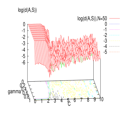
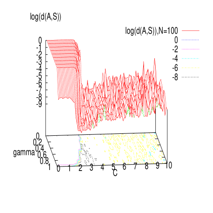
Figure 1: Fig. 1a. Average value of the distance $d({\cal A},{\cal S})$ versus $\gamma,C$, for $N=50$. Fig. 1b. $N=100$ (in $\log_{10}$ scale).

5.2 Adding noise to the dynamics.

It is usual in neural network modeling to add Brownian noise to the deterministic dynamics. This noise accounts for different effects such as the diffusion of neurotransmitters involved in the synaptic transmission, the degrees of freedom neglected by the model, external perturbations, etc … Though it is not evident that the “real noise” is Brownian, using this kind of perturbations has the advantage of providing a tractable model where standard theorems in the theory of stochastic processes FauTou or methods in non equilibrium statistical physics (e.g. Fokker-Planck equations BrunHak ) can be applied.

The addition of this type of noise to the dynamics of BMS model will result, in the region where $d(\Omega,{\cal S})$ is small, in an effective initial condition sensitivity and an effective positive Lyapunov exponent.

More precisely, consider a noisy version of (1).

$$V_{i}(t+1)=\gamma V_{i}(t)\left(1-Z[V_{i}(t)]\right)+\sum_{j=1}^{N}W_{ij}Z[V_{j}(t)]+I^{ext}_{i}(t)+B_{i}(t);\qquad i=1\dots N.$$ (49)

where ${\bf B}\stackrel{{\scriptstyle\rm def}}{{=}}\left\{B_{i}(t)\right\}_{i=1;t=0}^{N,\infty}$ is a Gaussian random process with zero mean and a covariance $Cov(B_{i}(t),B_{j}(s))=\sigma_{B}^{2}\delta_{t,s}\delta_{i,j}$. The probability distribution of the stochastic process ${\bf V}$, on a finite time horizon $T$, for a fixed realisation of the ${\cal W}$ can be obtained by using a discrete time version of Girsanov theorem Skor ,SC . From this, it is possible to estimate the probability that a trajectory approaches the singularity set ${\cal S}$ within a finite time $T$ and a distance $d$ by using Freidlin-Wentsel estimates FW . Also, eq. (27) is useful to estimate the measure of points having a local stable manifold. In this context one can compute the probability to approach the singularity set within a distance $\epsilon$; also one can construct a Markov chain for the transition between the attraction basin of the periodic orbits of the unperturbed dynamics. This will be done in a forthcoming paper.

5.3 Time dependent input.

One may also wonder what happens to the present analysis when a deterministic, time dependent external input, is imposed upon the dynamics (the case of a stochastic input is covered by eq. (49) above). Away from the singularity set ($d(\Omega,{\cal S})$ large) the effect of a time dependent input with a small amplitude (lower than $d(\Omega,{\cal S})$) will not be different from the case studied in the present paper. This is basically because a small input may be viewed as a perturbation of the trajectory, and the contraction properties of the dynamics will damp the perturbation as long as the trajectory stays away from the singularity set.

The situation is different if, at some place, the action of the time dependent input leads to a crossing of the singularity. This crossing can basically occur with a time independent input, but in the time dependent case there is a particularly salient effect, that may be easily revealed with periodic external currents. That is resonance effects. If the unperturbed trajectory has some typical recurrent time to come close to the singularity set, and if the time dependent perturbation is not synchronized with this recurrence time, one expects that the contraction effect will damp the perturbation with no clear cut “emergent” effect. On the other hand, if the period of the periodic signal is a multiple of the recurrence time, there may be a major effect. The result would be a frequency dependent response of the system exhibiting sharp peaks (resonance). This statement is actually more than a conjecture. Such resonances effects have indeed been exhibited in a recurrent discrete time neural network with firing rates JAB1 ,JAB2 ,JAB3 . It has been shown that applying a periodic input is a way to handle the interwoven effects of non linear dynamics and synaptic topology. Similar effects should be observed in BMS model.

5.4 Learning and synaptic plasticity.

What would be the effect of a synaptic weight variations (synaptic plasticity, LTD, LTP, STDP, Hebbian learning) on the dynamical system (1) ? These variations corresponds to moving the point corresponding to the dynamical system in the parameters space $({\cal W},{\bf I^{ext}})$. This motion is neither random nor arbitrary. Indeed, assume that one imposes to the neural network an input/stimulus ${\bf I^{ext}}=\left\{I^{ext}_{i}(t)\right\}$. $I^{ext}_{i}$ modifies directly the level of activity of neuron $i$, and acts indirectly on other neurons (provided that the synaptic graph is connected). A simple stimulus can therefore strongly modify the dynamics, the attracting set, the distance $d(\Omega,{\cal S})$, etc ….

In the case where ${\bf I^{ext}}$ does not depend on time, the following result follows directly from the analysis presented in this paper.

Theorem 5.1

For a generic set of values of $({\cal W},{\bf I^{ext}})$, there exists a finite partition of ${\cal M}=\bigcup{\cal D}_{n}$, such that $\forall{\bf V}\in{\cal D}_{n}$ the $\omega$-limit set of ${\bf V}$, $\omega({\bf V})$ is a stable periodic orbit, with a finite period. This orbit depends on ${\bf I^{ext}}$.

Proof

$\Omega$ is generically a finite union of periodic orbits with a finite period. Each of orbit $n$ has an attraction basin ${\cal D}_{n}$ and the attraction basins consitute a partition of ${\cal M}$. ∎

This orbit (resp. its coding) may be viewed as the dynamical response of the neural network to input ${\bf I^{ext}}$, whenever the initial conditions are chosen $\in{\cal D}_{n}$. In this way, the neural network associates to an input a dynamical pattern encoded in the spiking sequence of this periodic orbit. In the same way one can associate to a series of inputs a series of periodic orbits (resp. codes), each orbit being specifically related to an input. This property results directly from th. (5.1) without particular assumption on the $W_{ij}$’s.

However, there might exist a large number of domains ${\cal D}_{n}$ and a large number of possible responses (orbits). Moreover, an orbit can be complex, with a very long period. This is particularly true at the “edge of chaos”. Indeed, consider the case where the distance $d(\Omega,{\cal S})$ is small, when the input is present. Then, dynamics is indistinguishable from chaos and the dynamical “signature” of the input is a very complex orbit, requiring a very long time to be identified. In other words, if one imagine a layered structure where the present neural network acts as a retina and where another neural network is intended to identify the orbit and “recognize” the input, the integration time of the retina will be very long at the edge of chaos. On the opposite, one may expect that a learning phase allows this system to associate the input to an orbit with a simple structure (small period) allowing a fast identification of the input.

It has been shown, in the case of recurrent neural networks with a sigmoidal transfer function Dauce , that Hebbian learning leads to a reduction of chaos towards a less complex dynamics, permitting to associate a pattern to simple orbits. The same effect has been observed by BMS BMS applying an STDP like rule to the model (1). In both cases, it has been observed that a synaptic evolution (Hebb or STDP) leads to associate to the input a sequence of orbits whose complexity decreases during the synaptic weights evolution. In the present context, this suggests that $d(\omega({\bf V}),{\cal S})$ increases during this evolution (note that the evolution is entirely dependent on the initial condition, ${\bf V}$. ).

A related question is: how do the statistical properties of raster plots evolve during synaptic weights evolution ? This question, and more generally the effect of synaptic evolution on dynamics can be addressed using tools from dynamical systems theory, in the spirit of the present paper. This will be the subject of a forthcoming paper. However, in the next section we mention briefly how tools from ergodic theory (thermodynamic formalism) can be used.

5.5 Statistical properties of orbits.

As we saw, the dynamics of (1) is a rather complex and can be, from an experimental point of view, indistinguishable from chaos. Consequently, the study of the finite evolution of the membrane potential (resp. the spiking patterns sequence) does not tell us what will be the further evolution, whenever the time of observation is smaller than the characteristic time $T_{d}$ of eq. (34). In this sense, the system is producing entropy on a finite time horizon. Thus, provided that $d(\Omega,{\cal S})$ is sufficiently small, one can do “as if” the system were chaotic and use the tools for analysis of chaotic systems. This also holds when one adds noise on the dynamics. A particularly useful set of tools is provided by ergodic theory and the thermodynamic formalism. In this approach one is interested in the statistical behavior of orbits, characterized by a suitable set of probability measure. A natural choice are Gibbs measures in the sense of Sinai-Ruelle-Bowen SRB . In a forthcoming paper we indeed show that Gibbs measures arise naturally in BMS model. They come either from statistical inference principles where one tries to maximize the statistical entropy given a set of fixed given quantities such as correlations functions or mean firing rate (a prominent example of application of this principle is given in Schneid ). They also arise when one wants to study the effect of synaptic plasticity (learning, STDP) on the selection of orbits. In the context of BMS model one can show that Hebbian learning and STDP are related to a variational principle on the topological pressure, which is the analogon of free energy in statistical mechanics.

5.6 The limit $dt\to 0$.

In the definition of the BMS model, one uses a somewhat rough approximation consisting in approximating the differential equation of the Integrate and Fire model with a Euler scheme, and discretizing time. A central question is: what did we lose by doing this, and is the model still relevant as a neural network model ? As mentioned in the introduction, this requires developments done elsewhere CV . But we would like here to point out here a few remarks on this aspect.

• From the “biological” point of view the Integrate and fire model with continuous time is already a rough approximation where the characteristic time for the neuron response is set to zero. One can actually distinguish (at least) $3$ characteristic time scales in neuron dynamics descriptions based on differential equations. The “microscopic time” $dt$ corresponds somehow to the shortest time scale involved in the spike generation (e.g. microscopic mechanism leading to opening of ionic channels). The “reaction time” $\tau_{r}$ of the neuron corresponds to the time of raise and fall for the spike. If one focuses on spikes (and does not consider time averaging over sliding windows leading to the firing rate description) the last relevant time scale is the characteristic time $T$ required for the neural network to reach a stationary regime. One expects to have $dt<<\tau_{r}<<T$. In the IF model, however, the time reaction $\tau_{r}$ is considered to be instantaneous (thus $\tau_{r}\leq dt$). This leads to delicate problems for the definition of the time of firing and requires the introduction of the “$t^{-}$ notation”. Using a discrete time approximation allows to circumvent this problem and corresponds somehow to pose $dt=\tau_{r}=1$.

  One may reject this procedure a priori. Our philosophy is instead to extract as much results as possible from the discrete time spiking model and decide a posteriori what has been lost (or won).

• From the dynamical system point of view, the limit $dt\to 0$ raises two problems. On one hand, the trajectories become continuous. Then one may have situations where the trajectory accumulates on ${\cal S}$ and where a small variation of the $W_{ij}$’s is not able to remove the intersection (as it is the case in th. 3.3). This type of situation is known in the field of genetic networks (see Farcot and references therein). However, as mentioned in the paper, the situation is slightly different here, because of the neurons reset, leading to an infinite contraction of a domain onto a point. This effect really simplifies the dynamics study, and is still present in the continuous time case. However, this aspect would require careful investigations, not in the scope of the present work.

  The second problem is the use of a Euler scheme in the discretization. Using more elaborated schemes would complicate the analysis since the model would loose its convenient piecewise affine structure. We don’t know what this would add.

• Finally, from a numerical point of view, softwares use discrete time. One aspect that interests us particularly is to know what are actually the computing capacities of the discrete time model compared to classical IF models and how much has been lost.

- (1) Bak P. ”How Nature works: the science of Seld-Organized Criticality.”, Springer-Verlag (1996), Oxford University Press (1997).
- (2) Blanchard Ph., Cessac B. Krüger T., ”A dynamical system approach to SOC models of Zhang’s type.” Jour. of Stat. Phys., 88 (1997), 307-318.
- (3) Blanchard Ph., Cessac B., Krüger T., ”What can one learn about Self-Organized Criticality from Dynamical System theory ?” Jour. of Stat. Phys., 98 (2000), 375-404.
- (4) Cessac B., Blanchard Ph.,Krüger T., Meunier J.L., Journal of Statistical Physics, Vol. 115, No 516, 1283-1326 (2004).
- (5) Brunel, N. and Hakim, V. (1999).“Fast global oscillations in networks of integrate-and-fire neurons with low firing rates”. Neural Comput., 11:1621-1671.
- (6) Cessac B., Doyon B., Quoy M., Samuelides M., ”Mean-field equations, bifurcation map and route to chaos in discrete time neural networks”, Physica D, 74, 24-44, (1994).
- (7) Cessac B., ”Occurence of chaos and AT line in random neural networks”, Europhys. Let., 26 (8), 577-582, (1994).
- (8) Cessac B., ”Increase in complexity in random neural networks”, J. de Physique I (France), 5, 409-432, (1995).
- (9) B. Cessac, O. Mazet, M. Samuelides, H. Soula, ”Mean field theory for random recurrent spiking neural networks”, NOLTA’05 (Non Linear Theory and its Applications) October 18-21, 2005, Brugge, Belgium.
- (10) Cessac B., Samuelides M., (2007), ”From Neuron to Neural Networks dynamics. ”, EPJ Special Topics ”Topics in Dynamical Neural Networks : From Large Scale Neural Networks to Motor Control and Vision”.
- (11) Cessac B., Sepulchre J.A., “Stable resonances and signal propagation in a chaotic network of coupled units , Phys. Rev. E 70, 056111, (2004);
- (12) Cessac B., Sepulchre J.A., ”Transmitting a signal by amplitude modulation in a chaotic network ”, Chaos 16, 013104 (2006);
- (13) Cessac B., Sepulchre J.A., ”Linear Response in a class of simple systems far from equilibrium”, , Physica D, Volume 225, Issue 1 , Pages 13-28.
- (14) Cessac B., Viéville T. (2007), “Biological plausibility of discrete time spiking neural networks.”, submited.
- (15) Cessac B, Touboul J.. “A discrete time neural network model with spiking neurons: the case of random synapses.”, in preparation.
- (16) Chernov N., Markarian R., “Chaotic Billiards”, American Mathematical Society (2006).
- (17) Coutinho R., Fernandez B., Lima R., Meyroneinc A., “Discrete time piecewise affine models of genetic regulatory networks”, J. Math. Biology, 52, 524-570, (2006)
- (18) Dauce E., Quoy M., Cessac B., Doyon B. and Samuelides M. ”Self- Organization and Dynamics reduction in recurrent networks: stimulus presentation and learning”, Neural Networks, (11) , 521-533, (1998).
- (19) Derrida B., “Dynamical phaste transition in non-symmetric spin glasses”, Journal of Physics A: Mathematical and General 20: 721-725 (1987).
- (20) B. Derrida, H. Flyvbjerg, Multivalley structure in Kauffman’s model: analogy with spin glasses J. Phys. A19, L1003-L1008 (1986)
- (21) B. Derrida, Y. Pomeau, Random networks of automata: a simple annealed approximation, Europhys. Lett. 1, 45-49 (1986)
- (22) Eckmann J.P., Ruelle D., “Ergodic Theory of Strange attractors” Rev. of Mod. Physics, 57, 617,(1985).
- (23) Farcot E., “Etude d’une classe d’équations différentielles affines par morceaux modélisant des réseaux de régulation biologique”, Thèse de Doctorat, Grenoble, France (2005).
- (24) Faugeras O., Papadopoulo T., Touboul J., Bossy M., Tanre E., Talay D., ”The Statistics Of Spikes Trains For Some Simple Types Of Neuron Models”, Proceedings of the NeuroComp 2006 Conference, Pont-à-Mousson, France, (2006),
- (25) M. I. Freidlin and A. D. Wentzell, Random Perturbations of Dynamical Systems Springer, New York, (1998).
- (26) Gerstner W.,, Kistler W.M., “Spiking Neuron Models. Single Neurons, Populations, Plasticity” Cambridge University Press, (2002).
- (27) Guckenheimer J., Holmes Ph., “Non linear oscillations, dynamical systems, and bifurcation of vector fields.”, Springer-Verlag (1983).
- (28) Guikhman I., Skorhokod A., “Introduction à la théorie des processus aléatoires”, Editions Mir, Moscou (1980).
- (29) Hodgkin, A. L. and Huxley, A. F. . “Current carried by sodium and potassium ions through the membrane of the giant axon of Loligo.”. J. Physiol. (Lond.), 116: 449-472, (1952). Hodgkin, A. L. and Huxley, A. F. “A quantitative description of ion currents and its applications to conduction and excitation in nerve membranes.”. J. Physiol. (Lond.), 117:500-544, (1952).
- (30) Hunt, B. R., T. Sauer, and J. A. Yorke, ”Prevalence: A translation-invariant ‘almost every’ on infinite-dimensional spaces,” Bull. Am. Math. Soc. 27, 217–238, (1992).
- (31) Izhikevich E.M. “Simple Model of Spiking Neurons”. IEEE Transactions on Neural Networks, 14:1569- 1572, (2003).
- (32) SA Kauffman, J. Theor. Biol. 22 (1969).
- (33) Katok A., Hasselblatt B., “Introduction to the modern theory of dynamical systems”, Kluwer (1998).
- (34) Keller G., “Equilibrium states in ergodic theory”, Cambridge university press (1998)
- (35) Kruglikov B., Rypdal M. “ Entropy via multiplicity“, arXiv math.DS/0505019 ; Kruglikov B., Rypdal M. “A piece-wise affine contracting map with positive entropy” arXiv math.DS/0504187
- (36) Langton C.G., “Computation at the edge of chaos”, Physica D, 42:12-37 (1990).
- (37) Lima R., Ugalde E., “Dynamical complexity of discrete time regulatory networks”, NonLinearity 19, 237-259 (2006).
- (38) W. Maass and C. Bishop, “Pulsed Neural Networks”, MIT-Press (Cambridge), 1998.
- (39) Mézard M., Parisi G., Virasoro M.A., ”Spin-glass theory and beyond”, World scientific Singapore, (1987)
- (40) Packard N., “Adaptation towards the edge of chaos”. In Kelso J.A.S, Mandell A.J. and Shlesinger M.F. Editors, Dynamic patterns in complex systems. Pages 293-301. World Scientific (1988).
- (41) Parry W., Pollicott M. “Zeta functions and the periodic orbit structure of hyperbolic dynamics”, Collection Asterisque 187-188, Société Mathématique de France, (1990).
- (42) Rieke F., Warland D., de Ruyter van Steveninck R., Bialek W., “Spikes: exploring the neural code”, MIT Press (1999).
- (43) Roxin, N Brunel and D Hansel (2005), “The role of delays in shaping the spatio-temporal dynamics of neuronal activity in large networks”, Physical Review Letters, 94, 238103
- (44) Rudolph M., Destexhe A. (2006), “Analytical Integrate and Fire Neuron models with conductance-based dynamics for event driven simulation strategies”, Neural Computation 18, 2146-2210.
- (45) Sinai Ya. G. , “Gibbs measures in ergodic theory”, Russ. Math. Surveys, 27 No 4, 21-69, (1972); Ruelle D. “Thermodynamic formalism” (1978). Reading, Massachusetts: Addison-Wesley; Bowen R. “Equilibrium states and the ergodic theory of Anosov diffeomorphisms”, Lect. Notes.in Math.,, Vol. 470, Berlin: Springer-Verlag (1975).
- (46) Sherrington D., “An introduction and overview is given of the theory of spin glasses and its application”, cond-mat/9806289.
- (47) Sherrington D., Kirkpatrick S., ”Solvable model of spin glass”, Phys. Rev. Let. Vol 35, Num 26 (1975), 1792.
- (48) M. Samuelides, B. Cessac, ”Random Recurrent Neural Networks”, review paper, to appear in, Topics in Neural Networks.”, European Physical Journal (topical issue), Springer (2006)
- (49) Schneidman E., Berry M.J., Segev R., Bialek W., “Weak pairwise correlations imply strongly correlated network states in a neural population”, Nature 04701, Vol. 440, April 2006.
- (50) Soula H., “Dynamique et plasticité dans les réseaux de neurones à impulsions”, thèse de doctorat, INSA Lyon, 2005.
- (51) Soula H., Beslon G., Mazet O. ’Spontaneous dynamics of assymmetric random recurrent spiking neural networks’ Neural Computation 18:1 (2006)