Anomalous Hall effect in a two-dimensional electron gas

Abstract

The anomalous Hall effect in a magnetic two-dimensional electron gas with Rashba spin-orbit coupling is studied within the Kubo-Streda formalism in the presence of pointlike potential impurities. We find that all contributions to the anomalous Hall conductivity vanish to leading order in disorder strength when both chiral subbands are occupied. In the situation that only the majority subband is occupied, all terms are finite in the weak scattering limit and the total anomalous Hall conductivity is dominated by skew scattering. We compare our results to previous treatments and resolve some of the discrepancies present in the literature.

I Introduction

In 1879, Edwin Hall ran a current through a gold foil and discovered that a transverse voltage was induced when the film was exposed to a perpendicular magnetic field. Hall The ratio of this Hall voltage to the current density is the Hall resistivity. For paramagnetic materials, the Hall resistivity is proportional to the applied magnetic field and Hall measurements give information about the concentration of free carriers and determine whether they are holes or electrons. Magnetic films exhibit both this ordinary Hall response and an extraordinary or anomalous Hall response that does not disappear at zero magnetic field and is proportional to the internal magnetization: $R_{\rm Hall}=R_{o}H+R_{s}M$, where $R_{\rm Hall}$ is the Hall resistance, $R_{o}$ and $R_{s}$ are the ordinary and anomalous Hall coefficients, $M$ is the magnetization, and $H$ is the applied magnetic field. The anomalous Hall effect (AHE) is the consequence of spin-orbit coupling and allows an indirect measurement of the internal magnetization.

Despite the simplicity of the experiment, the theoretical basis of the AHE is still hotly debated and a source of conflicting reports. Sinova et al. (2004) Different mechanisms contribute to the AHE: an intrinsic mechanism and extrinsic mechanisms such as skew-scattering and side-jump contributions. The intrinsic mechanism is based solely on the topological properties of the Bloch states originating from the spin-orbit-coupled electronic structure as first suggested by Karplus and Luttinger. Karplus and Luttinger (1954) Their approach gives an anomalous Hall coefficient $R_{s}$ proportional to the square of the ordinary resistivity, since the intrinsic AHE itself is insensitive to impurities. The skew-scattering mechanism, as first proposed by Smit, Smit (1955); note_skew relies on an asymmetric scattering of the conduction electrons by impurities present in the material. Not surprisingly, this skew scattering contribution to $R_{s}$ is sensitive to the type and range of the scattering potential and, in contrast to the intrinsic mechanism, scales linearly with the diagonal resistivity. The presence of impurities also leads to a side-step type of scattering, which contributes to a net current perpendicular to the initial momentum. This is the so-called side-jump contribution, whose semi-classical interpretation was pointed out by Berger. Berger (1970) However, it is not trivial to correctly account for such contributions in the semiclassical procedure, making a connection to the microscopic approach very desirable.

The early theories of the AHE involved complex calculations with results that where not easy to interpret and often contradicting each other. Nozieres and Lewiner (1973) The adversity facing these theories stems from the origin of the AHE: it appears due to the interband coherence and not just due to simple changes in the occupation of Bloch states, as was recognized in the early works of Luttinger and Kohn. Kohn and Luttinger (1957); Luttinger (1958) Nowadays, most treatments of the AHE either use the semiclassical Boltzmann transport theory or the diagrammatic approach based on the Kubo-Streda linear-response formalism. The equivalence of these two methods for the two-dimensional Dirac-band graphene system has recently been shown by Sinitsyn et al., Sinitsyn et al. (2006) who explicitly identified various diagrams of the more systematic Kubo-Streda treatment with the physically more transparent terms of the semiclassical Boltzmann approach.

It is therefore important to also obtain a similarly cohesive understanding of the AHE in other systems such as the two-dimensional (2D) spin-polarized electron gas with Rashba spin-orbit interaction in the presence of pointlike potential impurities, where a series of previous studies has led to a multitude of results with discrepancies arising from the focus on different limits and/or subtle missteps in the calculations. Culcer (2003); Dugaev et al. (2005); Sinitsyn et al. (2005); Liu and Lei (2005, 2005); ichiro Inoue et al. (2006); Onoda et al. (2006) It is the purpose of this paper to review and analyze the previous attempts and to provide a detailed analysis of all contributions to the AHE in a two-dimensional electron gas. Since we have already demonstrated the equivalence of the Kubo-Streda formalism and the semiclassical Boltzmann approach with respect to skew scattering in the two-dimensional electron gas in a previous paper, Borunda:2007_a we will focus here exclusively on the diagrammatic formalism based on the Kubo-Streda treatment.

The outline of the article is as follows. We start by reviewing and commenting on previous studies of the AHE in the two-dimensional electron gas in Sec. II, where we compare them with our results and discuss the discrepancies and their possible origins. In Sec. III we present details of our calculation within the diagrammatic Kubo-Streda formalism. In Sec. III.3 we provide simple analytical limits of all terms of the anomalous Hall conductivity and discuss the full evaluation in Sec. III.4. Finally, in Sec. IV we present our conclusions.

II Comparison with previous approaches

Currently there are several publications on the AHE in two dimensional systems reaching different quantitative predictions even in the same limits. Culcer (2003); Dugaev et al. (2005); Sinitsyn et al. (2005, 2006); Liu and Lei (2005, 2005); ichiro Inoue et al. (2006); Onoda et al. (2006) In the present paper we present a calculation with conclusions that are in disagreement with some previous studies. On such a background we believe that previous articles have to be discussed in some details. Below we review the history of the problem and explain why we think the subject has to be reconsidered.

A first study of the AHE in two dimensional systems was done by Culcer et al., Culcer (2003) who calculated only the intrinsic contribution to the Hall conductivity for a wide class of two-dimensional systems, including the Rashba two-dimensional electron gas as a special case. The intrinsic contribution plays a special role in the theory of the AHE because it is not related to the scattering of electrons but is rather caused by the unusual trajectories of electrons under the action of the electric field. However, the disorder contributions can also be important and further insight was needed in the quest for a quantitatively rigorous theory of the dc-AHE.

The first attempts to understand the disorder effects where done independently by two groups, Dugaev et al. (2005); Sinitsyn et al. (2005) each employing different approaches. Dugaev et. al. Dugaev et al. (2005) used the version of the Kubo formula, which expresses the Hall conductivity in terms of the causal Green functions. The intrinsic contribution appears as a result of calculations with bare Green functions, while disorder effects renormalize the quasi-particle life time and the current vertex. This approach is formally rigorous and is similar to the one we adopt in our work. However, our final results are quantitatively different from those found in Ref. Dugaev et al., 2005 due to a subtlety in the calculation of the vertex at the Fermi surface which was later corrected in the appendix of Ref. Sinitsyn et al., 2006. Starting with the equation for the renormalized vertex $T_{x}=ak_{x}+b\sigma_{x}+c\sigma_{y}$ and with the assumption that the density of impurities is low, they find correctly that $b=0$ to leading order in $n_{i}$, i.e. $a/b\propto n_{i}$. However, such a term gets multiplied by an equivalent divergent term within the Kubo formula leading to a non-zero contribution to the AHE conductivity to zeroth order in $n_{i}$.

In contrast to the previous quantum mechanical approach, Sinitsyn et al. Sinitsyn et al. (2005) employed the semiclassical wave-packet approach focusing only on the understanding of the side-jump contribution and formulating the semi-classical problem in a gauge invariant form. This work Sinitsyn et al. (2005) intentionally avoids a discussion of the skew-scattering contribution due to the asymmetry of the collision term kernel, which is also an important mechanism of the Hall current and can even be parametrically similar to all other contribution Sinitsyn et al. (2006) in the case of Gaussian correlations. Therefore, the work in Ref. Sinitsyn et al., 2005 is meant as an intuitive introduction into the physics of the anomalous velocity and the side-jump effect, but does not offer a rigorous quantitative comparison even in the considered limit of smooth disorder potential.

Subsequently two papers by Liu et al. Liu and Lei (2005, 2005) studied the problem using the Keldysh technique for linear transport. The Keldysh technique leads to the quantum Boltzmann equation for the diagonal elements of the density matrix in momentum space when only elastic scattering events are considered. In the steady state limit of a weak electric field this equation can be written as follows:

$$e{\bf E\cdot}\nabla_{{\bf p}}\hat{\rho}({\bf p})+i[\hat{H}_{0},\hat{\rho}({\bf p})]=\hat{I}_{\mathrm{c}ol}(\hat{\rho}({\bf p}))\,,$$ (1)

where $\hat{I}_{\mathrm{c}ol}$ contains all disorder dependent terms that become zero when $\hat{\rho}({\bf p})$ is the density matrix in thermodynamic equilibrium and $\hat{H}_{0}$ is the disorder free part of the Hamiltonian. The “hat” means that $\hat{\rho}$ and $\hat{I}_{col}$ are matrices in the band index space. The term containing the electric field is called the driving term. In the linear-response approximation it only depends on the equilibrium part of the density matrix.

To start with Eq. (1) is correct and is also the starting point of the pioneering work by Luttinger Luttinger (1958) and therefore one can compare it directly with steps taken by Liu et al. Liu and Lei (2005, 2005) Luttinger’s approach was to split the density matrix into equilibrium and nonequilibrium parts $\hat{\rho}=\hat{\rho}_{\mathrm{e}q}+\hat{\rho}_{\mathrm{n}eq}$ where $\hat{\rho}_{\mathrm{n}eq}$ is linear in electric field. It is this part of the density matrix that is responsible for nonzero currents. For weak disorder potential $\hat{V}$, Luttinger looked for $\hat{\rho}_{\mathrm{n}eq}$ as a series in powers of the disorder potential. He found that this series starts from the term of the order $\hat{V}^{-2}$

$$\hat{\rho}_{\mathrm{n}eq}=\hat{\rho}_{\mathrm{n}eq}^{(-2)}+\hat{\rho}_{\mathrm{n}eq}^{(-1)}+\hat{\rho}_{\mathrm{n}eq}^{(0)}+\cdots$$ (2)

As pointed out by Luttinger, the leading order term $\hat{\rho}_{\mathrm{n}eq}^{(-2)}$ does not contribute to the Hall effect and is only responsible for the longitudinal diffusive current. The term $\hat{\rho}_{\mathrm{n}eq}^{(-1)}$ was identified with skew scattering. This term, however, is parametrically very distinct and vanishes in the approximation of purely Gaussian correlations of disorder Fourier components; therefore, Luttinger went to next order and calculated the term $\hat{\rho}_{\mathrm{n}eq}^{(0)}$. He found a number of contributions, whose physical meaning he did not clarify. The main conclusion was that at this order both the diagonal and off-diagonal parts of the density matrix become nonzero and contribute to the Hall conductivity, which becomes formally independent on the strength of disorder $\hat{V}$ in the DC limit, although disorder has to be included in the intermediate calculations.

Comparing this with the first work of Liu and Lei Liu and Lei (2005) we find that they determined self-consistently only the off-diagonal part of the density matrix in band index. This is, however, not enough for a rigorous quantitative result because the diagonal part of the $\hat{\rho}_{neq}^{(0)}$ contribution has been known to be important since Luttinger’s pioneering work.

In their next effort Liu et al. Liu and Lei (2005) studied the problem of 2D Rashba systems in small gap semiconductor materials, in which a projection to the conduction band leads to extrinsic type spin-dependent contributions. In this work they noticed that the diagonal part is important and calculated it numerically. For the driving term in Eq. (1) Liu et al. assume that $\hat{\rho}_{eq}$ is just a diagonal equilibrium Fermi distribution. This would be correct if one was using the basis of the eigenstates of the full Hamiltonian with impurities. However, both Liu et al. and Luttinger work in the chiral basis of the disorder free Hamiltonian $\hat{H}_{0}$. In this basis the equilibrium state density matrix is no longer diagonal and can also be written as a series in powers of the disorder potential:

$$\hat{\rho}_{eq}=\hat{\rho}_{eq}^{(0)}+\hat{\rho}_{eq}^{(2)}+\cdots$$ (3)

Luttinger has shown that in order to properly evaluate the non-equilibrium part $\hat{\rho}_{neq}^{(0)}$ one should include the second term $\hat{\rho}_{eq}^{(2)}$ of the expansion of the equilibrium density matrix in Eq. (3) into the driving term of Eq. (1). This was not done in Ref. Liu and Lei, 2005 and therefore we believe that their work is incomplete due to such omission. We also note that the correction of order $\hat{V}^{2}$ in Eq. (3) leads to the Hall current contribution, which was identified in the semiclassical approach Sinitsyn:2006_a as the anomalous distribution correction and if omitted leads to errors of factors of two in the typical side-jump type contributions.Nozieres and Lewiner (1973) In the Kubo formula approach, neglecting this correction would be equivalent to the unjustified omission of an important subset of Feynman diagrams. Sinitsyn et al. (2006) Within the calculation presented here all these terms are present.

Inoue et al. ichiro Inoue et al. (2006) calculated the AHE contribution using the same approach we use focusing on the limit of both subbands being occupied and, in addition to the disorder that we consider, incorporating magnetic impurities in the model Hamiltonian. They found that for paramagnetic impurities the Hall conductivity vanishes. Our more general calculations confirm this result. However, we point to one important difference in its derivation. In both cases the dc-limit Kubo formula, where the conductivity is expressed via retarded and advanced Greens functions, has been employed to calculate the Hall conductivity. As was shown by Streda  Streda (1982), this version of the Kubo formula contains two parts: $\sigma^{I}_{xy}$ a contribution from the Fermi surface and $\sigma^{II}_{xy}$ a contribution from all states of the Fermi sea. The latter part is less known because it does not appear in the expression for the longitudinal conductivity. Inoue et al. ichiro Inoue et al. (2006) calculated only $\sigma^{I}_{xy}$ and indeed we find that for their choice of parameters the second part of the conductivity $\sigma^{II}_{xy}$ vanishes, explaining the agreement with our results. In a more general analysis, beyond the limit of weak spin-orbit and Zeeman couplings, we find a non-vanishing $\sigma^{II}_{xy}$. Our work provides the missing estimate of $\sigma^{II}_{xy}$ and extends the calculations of Inoue et al. ichiro Inoue et al. (2006)

Finally, the latest work on the subject is by Onoda et al. Onoda et al. (2006) The authors used the Keldysh technique, which they reformulated in a way appropriate for multiband problems in a gauge invariant formalism. They also derived a self-consistent equation, which is the analog of the standard quantum Boltzmann equation and solved it numerically. Unfortunately, lacking a full understanding of the details of the numerical procedure and the starting equations being very formal within a non-chiral basis, a detailed discussion of their approach cannot be performed here. However, being devoted to the same model, the final results can be compared directly with the possible discrepancies arising from the different limits considered in the disorder distributions in which $n_{i}$ and the disorder strength are two independent parameters in their calculations. Onoda et al. Onoda et al. (2006) find a strong skew scattering contribution of the order of $\epsilon_{SO}V_{\mathrm{i}mp}\sigma_{xx}/W^{2}$, where $W$ is the inverse density of states. The skew scattering term changes sign at the point where the minority band becomes depleted, which they call the resonance point. The authors find also that the side-jump contribution is small in comparison with the intrinsic one. Our results confirm neither of those predictions. We find that for the Rashba model with randomly placed delta-function impurities the leading part of the skew-scattering vanishes identically when the Fermi level is above this resonance point. Although skew scattering could still appear in higher order terms of the Born series, we expect these contributions to be small because they are of higher order in $V_{\mathrm{i}mp}$. On the other hand, Onoda et al Onoda et al. (2006) consider the limit of dilute impurities $n_{i}\rightarrow 0$ independently of the disorder strength $V_{\mathrm{i}mp}$ which might be the origin for the discrepancies. Using the Keldysh formalism in the disorder free basis we have been able to verify analytically our results. Further numerical analysis Kovalev:2007_b of different limits will be necessary to settle the discrepancies with the results by Onoda et al. Onoda et al. (2006)

III Anomalous Hall conductivity of the 2DEG

III.1 Model Hamiltonian

We consider a spin-polarized two dimensional electron gas with Rashba spin-orbit interaction

$$H=\frac{k^{2}}{2m}\sigma_{0}+\alpha(\sigma_{x}k_{y}-\sigma_{y}k_{x})-h\sigma_{z}+V({\bf r})\sigma_{0}$$ (4)

where $m$ is the the effective in-plane mass of the quasiparticles, $\alpha$ the spin-orbit coupling parameter, $h$ the exchange field, and $\sigma_{i}$ the $2\times 2$ Pauli matrices. The eigenenergies of the clean system are

$$E_{k\pm}=\frac{k^{2}}{2m}\pm\lambda_{k}\quad{\rm with}\quad\lambda_{k}=\sqrt{h^{2}+\alpha^{2}k^{2}}$$ (5)

and are shown in Fig. 1. The retarded Greens function of the clean system is:

$$G^{(0)R} = \frac{\left(\omega-\frac{k^{2}}{2m}+i0^{+}\right)\sigma_{0}+\alpha k_{y}\sigma_{x}-\alpha k_{x}\sigma_{y}-h\sigma_{z}}{\left(\omega-\frac{k^{2}}{2m}+i0^{+}\right)^{2}-h^{2}-\alpha^{2}k^{2}}$$ (6)

$$= G^{(0)R}_{0}\sigma_{0}+G^{(0)R}_{x}\sigma_{x}+G^{(0)R}_{y}\sigma_{y}+G^{(0)R}_{z}\sigma_{z}\,,$$

with

$$G^{(0)R}_{0}\!\!\! = \!\!\!\frac{1}{2}(G^{(0)}_{+}\!\!+G^{(0)}_{-})\,\,\,\,\,G^{(0)R}_{z}\!=\!-\frac{1}{2}\frac{h}{\lambda_{k}}(G^{(0)}_{+}\!\!-G^{(0)}_{-})$$ (7)

$$G^{(0)R}_{x}\!\!\! = \!\!\!\frac{1}{2}\frac{\alpha k_{y}}{\lambda_{k}}(G^{(0)}_{+}\!\!-G^{(0)}_{-})\,\,\,\,\,G^{(0)R}_{y}\!=\!-\frac{1}{2}\frac{\alpha k_{x}}{\lambda_{k}}(G^{(0)}_{+}\!\!-G^{(0)}_{-})$$

and

$$G^{(0)}_{\pm}=\frac{1}{\omega-E_{k\pm}+i0^{+}}\,.$$ (8)

The disorder potential $V(\mbox{\bf r})$ in Eq. (4) is assumed as spin-independent. We consider the model of randomly located $\delta$-function scatterers: $V({\bf r})=\sum_{i}V_{i}\delta({\bf r}-{\bf R}_{i})$ with random and strength distributions satisfying $\langle V_{i}\rangle_{\mathrm{d}is}=0$, $\langle V_{i}^{2}\rangle_{\mathrm{d}is}=V_{0}^{2}\neq 0$ and $\langle V_{i}^{3}\rangle_{\mathrm{d}is}=V_{1}^{3}\neq 0$. This model is different from the standard white noise disorder model in which only the second order cumulant is nonzero; $\langle|V^{0}_{{\bf k^{\prime}k}}|^{2}\rangle_{dis}=n_{i}V_{0}^{2}$ where $n_{i}$ is the impurity concentration and other correlators are either zero or related to this correlator by Wick’s theorem. The deviation from white noise in our model is quantified by $V_{1}\neq 0$ and is necessary to capture part of the skew scattering contribution to the anomalous Hall effect.

We calculate the self-energy using the Born approximation:

$$\Sigma^{R} = -i(\Gamma\sigma_{0}+\Gamma_{z}\sigma_{z})$$

$$= \!\!\!-\frac{i}{4}n_{i}V_{0}^{2}\left((\nu_{+}+\nu_{-})\sigma_{0}-h\left(\frac{\nu_{+}}{\lambda_{+}}-\frac{\nu_{-}}{\lambda_{-}}\right)\sigma_{z}\right)$$

where $\nu_{\pm}$ is related to the density of states at the Fermi levels of the two subbands

$$\nu_{\pm}=k\left|\frac{dE_{k\pm}}{dk}\right|^{-1}=\frac{m\lambda_{\pm}}{\sqrt{\lambda_{F}^{2}+(\alpha^{2}m)^{2}}}$$ (10)

with

$$\lambda_{\pm}=\sqrt{h^{2}+\alpha^{2}k_{\pm}^{2}}=\sqrt{\lambda_{F}^{2}+(\alpha^{2}m)^{2}}\mp\alpha^{2}m\,,\quad$$ (11)

where $\lambda_{F}=\sqrt{h^{2}+2\alpha^{2}m\epsilon_{F}}$ and

$$k_{\pm}=\sqrt{2m\left(\epsilon_{F}+\alpha^{2}m\mp\sqrt{\lambda_{F}^{2}+(\alpha^{2}m)^{2}}\right)}$$ (12)

are the Fermi momenta of the two subbands.

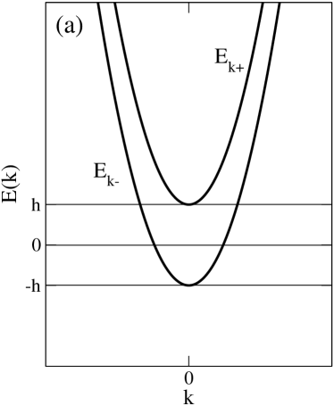
Figure 1: Single particle dispersion for small spin-orbit interaction $\alpha k_{F}/h=0.2$ (a) and large spin-orbit interaction $\alpha k_{F}/h=2.0$ (b).

Including the self-energy, the impurity averaged Greens function becomes:

$$G^{R}\!\!\! = \!\!\frac{\!\left(\omega-\frac{k^{2}}{2m}+i\Gamma\right)\sigma_{0}+\alpha k_{y}\sigma_{x}-\alpha k_{x}\sigma_{y}-(h+i\Gamma_{z})\sigma_{z}}{\left(\omega-\frac{k^{2}}{2m}+i\Gamma\right)^{2}-(h+i\Gamma_{z})^{2}-\alpha^{2}k^{2}}$$ (13)

$$= \!\!G^{R}_{0}\sigma_{0}+G^{R}_{x}\sigma_{x}+G^{R}_{y}\sigma_{y}+G^{R}_{z}\sigma_{z}\,.$$

By comparing this expression with Eq. (6) one observes that the impurity averaged Greens function can be obtained from the Greens function of the clean system by the following replacements:

$$\omega\to\omega+i\Gamma\,,\quad h\to h+i\Gamma_{z}\,.$$ (14)

In the limit of small $\Gamma_{z}$ one can therefore expand

$$\lambda_{k}\to\sqrt{(h+i\Gamma_{z})^{2}+\alpha^{2}k^{2}}\approx\lambda_{k}\left(1+i\frac{h\Gamma_{z}}{\lambda_{k}^{2}}\right)\,.$$ (15)

Using this approximation the impurity averaged Greens function can also be written as:

$$G^{R}_{0} = \frac{1}{2}(G^{R}_{+}+G^{R}_{-})$$ (16)

$$G^{R}_{x} = \sin\phi\,\tilde{G}^{R}_{x}=\frac{1}{2}\frac{\alpha k_{y}\lambda_{k}}{\lambda_{k}^{2}+i\Gamma_{z}h}(G^{R}_{+}-G^{R}_{-})$$

$$G^{R}_{y} = \cos\phi\,\tilde{G}^{R}_{y}=-\frac{1}{2}\frac{\alpha k_{x}\lambda_{k}}{\lambda_{k}^{2}+i\Gamma_{z}h}(G^{R}_{+}-G^{R}_{-})$$

$$G^{R}_{z} = -\frac{1}{2}\frac{\lambda_{k}(h+i\Gamma_{z})}{\lambda_{k}^{2}+i\Gamma_{z}h}(G^{R}_{+}-G^{R}_{-})$$

with

$$G^{R}_{\pm}=\frac{1}{\omega-E_{k\pm}+i\Gamma_{\pm}}$$ (17)

and

$$\Gamma_{\pm}=\Gamma\mp\Gamma_{z}\frac{h}{\lambda_{\pm}}\,.$$ (18)

III.2 General expression for the anomalous Hall conductivity

According to the Kubo-Streda formalism Streda (1982) the off-diagonal conductivity can be written as:

$$\sigma_{yx}=\sigma_{yx}^{I(a)}+\sigma_{yx}^{I(b)}+\sigma_{yx}^{II}$$ (19)

where

$$\sigma_{yx}^{I(a)}\!\! = \!\!\frac{e^{2}}{2\pi V}{\rm Tr}\langle v_{y}G^{R}(\epsilon_{F})v_{x}G^{A}(\epsilon_{F})\rangle$$ (20)

$$\sigma_{yx}^{I(b)}\!\! = \!\!-\frac{e^{2}}{4\pi V}{\rm Tr}\langle v_{y}G^{R}(\epsilon_{F})v_{x}G^{R}(\epsilon_{F})$$

$$\hskip 34.14322pt+v_{y}G^{A}(\epsilon_{F})v_{x}G^{A}(\epsilon_{F})\rangle$$

$$\sigma_{yx}^{II}\!\! = \!\!\frac{e^{2}}{4\pi V}\int_{-\infty}^{\infty}d\epsilon f(\epsilon){\rm Tr}\langle v_{y}G^{R}(\epsilon)v_{x}\frac{\partial G^{R}(\epsilon)}{\partial\epsilon}$$

$$-v_{y}\frac{\partial G^{R}(\epsilon)}{\partial\epsilon}v_{x}G^{R}(\epsilon)-v_{y}G^{A}(\epsilon)v_{x}\frac{\partial G^{A}(\epsilon)}{\partial\epsilon}$$

$$+v_{y}\frac{\partial G^{A}(\epsilon)}{\partial\epsilon}v_{x}G^{A}(\epsilon)\rangle\,.$$

Here, $\sigma^{I}$ results from the electrons at the Fermi surface whereas $\sigma^{II}$ denotes the contribution of all states of the Fermi sea. For $\sigma^{I(b)}$ and $\sigma^{II}$ it is sufficient to calculate the bare bubble contribution in the weak scattering limit Sinitsyn et al. (2006) because vertex corrections are of higher order in the scattering rate $\Gamma$. Plugging in the Greens function of Eq. (16) and using the velocity vertices

$$v_{x}=\frac{k_{x}}{m}\sigma_{0}-\alpha\sigma_{y}\,,\quad v_{y}=\frac{k_{y}}{m}\sigma_{0}+\alpha\sigma_{x}\,$$ (21)

one finds that $\sigma^{I(b)}$ vanishes

$$\sigma_{yx}^{I(b)} = -\frac{e^{2}}{4\pi V}\frac{1}{(2\pi)^{2}}\int d^{2}k\left(-i\alpha^{2}G_{0}^{R}G_{z}^{R}+i\alpha^{2}G_{z}^{R}G_{0}^{R}\right.$$ (22)

$$\left.-i\alpha^{2}G_{0}^{A}G_{z}^{A}+i\alpha^{2}G_{z}^{A}G_{0}^{A}\right)=0\,.$$

The bare contribution of $\sigma^{II}$ in the clean limit, i.e., for $\Gamma_{+}=\Gamma_{-}=0^{+}$ can be calculated by integration (see App. A) and yields

$$\sigma_{yx}^{II}\!=\!\frac{e^{2}}{4\pi}\!\left(\!\!1\!-\!\frac{h}{\sqrt{h^{2}+2\alpha^{2}m\epsilon_{F}+(\alpha^{2}m)^{2}}}\!\right)\!\!\Theta(h-\epsilon_{F})$$ (23)

where $\partial G_{\pm}^{R/A}/\partial\epsilon=-(G_{\pm}^{R/A})^{2}$ has been used. Including the real scattering rates $\Gamma_{+}$ and $\Gamma_{-}$ does not lead to qualitatively different results but mainly causes a slight smearing. Thus we consider it as sufficient to focus on the clean limit contribution of $\sigma^{II}$.

For $\sigma^{I(a)}$ vertex corrections can be of similar magnitude as the bare bubble and thus have to be considered carefully. In the weak scattering limit contributions of higher order impurity scattering vertices are small leaving only ladder type vertex corrections and the $V_{1}^{3}/(n_{i}V_{0}^{4})$ skew scattering contribution as the important terms. Borunda:2007_a Thus we decompose $\sigma^{I(a)}$ in the following way:

$$\sigma_{yx}^{I(a)}=\sigma_{yx}^{I(a),b}+\sigma_{yx}^{I(a),l}+\sigma_{yx}^{I(a),s}\,,$$ (24)

where $\sigma_{yx}^{I(a),b}$ is the bare bubble contribution (Fig. 2(a)), $\sigma_{yx}^{I(a),l}$ the ladder vertex corrections (Fig. 2(b)), and $\sigma_{yx}^{I(a),s}$ the skew scattering contribution (Fig. 2(c)). With respect to the skew scattering contribution we have shown Borunda:2007_a that only the diagrams with a single third order vertex (see Fig. 2(c)) contribute to order $V_{1}^{3}/(n_{i}V_{0}^{4})$. In this diagram both vertices have to be renormalized by ladder vertex corrections.

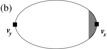
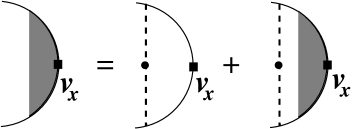
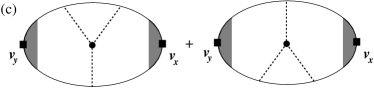
Figure 2: Diagrammatic representation of the bare bubble (a), of the ladder vertex corrections (b) and of the skew scattering contribution (c).

III.2.1 Bare bubble

The calculation of the bare bubble contribution proceeds as follows:

$$\sigma_{yx}^{I(a),b}=\frac{e^{2}}{2\pi}\!\!\int\!\!\!\int\frac{dkkd\phi}{(2\pi)^{2}}{\rm Tr}[v_{y}G^{R}(\epsilon_{F})v_{x}G^{A}(\epsilon_{F})]$$ (25)

$$=2i\alpha\!\!\int\!\!\frac{dkk}{2\pi}\left(\frac{k}{m}(\tilde{G}_{y}^{R}G_{z}^{A}-G_{z}^{R}\tilde{G}_{y}^{A})-\alpha(G_{0}^{R}G_{z}^{A}-G_{z}^{R}G_{0}^{A})\right)$$

$$=2i\alpha(2I_{3}-\alpha I_{2})$$

where (for explicit evaluation of integrals $I_{1}$, $I_{2}$, $I_{3}$ and $I_{4}$ see App. B)

$$I_{1}=\frac{1}{2\pi}\int dkk\left(G_{0}^{R}G_{0}^{A}-G_{z}^{R}G_{z}^{A}\right)$$ (26)

$$\approx\frac{1}{8}\left(\left(1-\frac{h^{2}}{\lambda_{+}^{2}}\right)\frac{\nu_{+}}{\Gamma_{+}}+\left(1-\frac{h^{2}}{\lambda_{-}^{2}}\right)\frac{\nu_{-}}{\Gamma_{-}}\right)$$

$$I_{2}=\frac{1}{2\pi}\int dkk\left(G_{0}^{R}G_{z}^{A}-G_{z}^{R}G_{0}^{A}\right)$$

$$\approx-\frac{i}{4}\left(\frac{\nu_{+}h}{\lambda_{+}^{2}}+\frac{\nu_{-}h}{\lambda_{-}^{2}}-\frac{\Gamma_{z}}{\Gamma_{+}}\frac{\nu_{+}\alpha^{2}k_{+}^{2}}{\lambda_{+}^{3}}+\frac{\Gamma_{z}}{\Gamma_{-}}\frac{\nu_{-}\alpha^{2}k_{-}^{2}}{\lambda_{-}^{3}}\right)$$

$$I_{3}=\frac{1}{2\pi}\int dk\frac{k^{2}}{2m}\left(\tilde{G}_{y}^{R}G_{z}^{A}-G_{z}^{R}\tilde{G}_{y}^{A}\right)$$

$$\approx-\frac{i}{4}\alpha\Gamma_{z}\left(\frac{\nu_{+}}{\Gamma_{+}\lambda_{+}}\left(\frac{\epsilon_{F}}{\lambda_{+}}-1\right)+\frac{\nu_{-}}{\Gamma_{-}\lambda_{-}}\left(\frac{\epsilon_{F}}{\lambda_{-}}+1\right)\right)$$

$$I_{4}=\frac{1}{2\pi}\int dk\frac{k^{2}}{2m}\left(G_{0}^{R}\tilde{G}_{y}^{A}+\tilde{G}_{y}^{R}G_{0}^{A}\right)$$

$$\approx-\frac{1}{4}\alpha\left(\epsilon_{F}\left(\frac{\nu_{+}}{\Gamma_{+}\lambda_{+}}-\frac{\nu_{-}}{\Gamma_{-}\lambda_{-}}\right)-\left(\frac{\nu_{+}}{\Gamma_{+}}+\frac{\nu_{-}}{\Gamma_{-}}\right)\right)\,.$$

III.2.2 Ladder diagrams

For the ladder terms $\sigma_{yx}^{I(a),l}$ we sum the vertex corrections in front of the $v_{x}$ vertex as indicated in Fig. 2(b). Starting from the momentum integrated bare velocity vertex

$$\!\!\int\!\!\!\int\frac{dkkd\phi}{(2\pi)^{2}}G^{R}(\epsilon_{F})v_{x}G^{A}(\epsilon_{F})=\gamma_{x}\sigma_{x}+\gamma_{y}\sigma_{y}\,,$$ (27)

with

$$\gamma_{x}=i(I_{3}-\alpha I_{2})\,,\quad\gamma_{y}=I_{4}-\alpha I_{1}$$ (28)

one finds for the renormalized vertex

$$\Gamma_{v_{x}} = \Gamma_{x}\sigma_{x}+\Gamma_{y}\sigma_{y}$$

$$= \gamma_{x}\sigma_{x}+\gamma_{y}\sigma_{y}$$

$$+n_{i}V_{0}^{2}\!\!\int\!\!\!\int\frac{dkkd\phi}{(2\pi)^{2}}G^{R}(\epsilon_{F})(\gamma_{x}\sigma_{x}+\gamma_{y}\sigma_{y})G^{A}(\epsilon_{F})$$

$$= \gamma_{x}\sigma_{x}+\gamma_{y}\sigma_{y}$$

$$+n_{i}V_{0}^{2}\left((I_{1}\Gamma_{x}+iI_{2}\Gamma_{y})\sigma_{x}+(I_{1}\Gamma_{y}-iI_{2}\Gamma_{x})\sigma_{y}\right)$$

and thus

$$\begin{pmatrix}\Gamma_{x}\\ \Gamma_{y}\end{pmatrix} = \frac{1}{(1-n_{i}V_{0}^{2}I_{1})^{2}-(n_{i}V_{0}^{2}I_{2})^{2}}$$

$$\begin{pmatrix}1-n_{i}V_{0}^{2}I_{1}&in_{i}V_{0}^{2}I_{2}\\ -in_{i}V_{0}^{2}I_{2}&1-n_{i}V_{0}^{2}I_{1}\end{pmatrix}\begin{pmatrix}\gamma_{x}\\ \gamma_{y}\end{pmatrix}\,.$$

The ladder diagrams are therefore given by

$$\sigma_{yx}^{I(a),l}\!\!\! = \!\!\!\frac{e^{2}}{2\pi}\!\!\int\!\!\!\!\!\int\!\frac{dkkd\phi}{(2\pi)^{2}}{\rm Tr}[G^{A}\!(\epsilon_{F})v_{y}G^{R}\!(\epsilon_{F})(\Gamma_{x}\sigma_{x}\!+\!\Gamma_{y}\sigma_{y})]$$

$$= \!\!\!-\frac{e^{2}}{2\pi}2(\gamma_{y}\Gamma_{x}+\gamma_{x}\Gamma_{y})$$

$$= \!\!\!-\frac{e^{2}}{\pi}\frac{n_{i}V_{0}^{2}\!\left(2\gamma_{x}\gamma_{y}(1\!\!-\!\!n_{i}V_{0}^{2}I_{1})\!\!+\!in_{i}V_{0}^{2}I_{2}(\gamma_{y}^{2}\!\!-\!\!\gamma_{x}^{2})\right)}{(1-n_{i}V_{0}^{2}I_{1})^{2}-(n_{i}V_{0}^{2}I_{2})^{2}}\,.$$

In the weak scattering limit this reduces to

$$\sigma_{yx}^{I(a),l}=-\frac{e^{2}}{\pi}\frac{n_{i}V_{0}^{2}\!\left(2\gamma_{x}\gamma_{y}(1\!\!-\!\!n_{i}V_{0}^{2}I_{1})\!\!+\!in_{i}V_{0}^{2}I_{2}\gamma_{y}^{2}\right)}{(1-n_{i}V_{0}^{2}I_{1})^{2}}\,.$$ (32)

III.2.3 Skew scattering

For skew scattering we consider only diagrams with a single third order impurity vertex and both external current vertices renormalized by ladder vertex corrections as indicated in Fig. 2(c). In analogy to the renormalized $v_{x}$-vertex in Eq. (III.2.2) also the renormalized $v_{y}$-vertex can be calculated and expressed via $\Gamma_{x}$ and $\Gamma_{y}$ as

$$\Gamma_{v_{y}}=-\Gamma_{y}\sigma_{x}-\Gamma_{x}\sigma_{y}\,.$$ (33)

Using these expressions the skew scattering diagram of Fig. 2(c) yields

$$\sigma_{yx}^{I(a),s}\!\!\! = \!\!\frac{e^{2}}{2\pi}\frac{n_{i}V_{1}^{3}}{2\pi}\!\!\!\int\!\!dkk{\rm Tr}[\Gamma_{v_{y}}G^{R}(\epsilon_{F})\Gamma_{v_{x}}\!\!+\Gamma_{v_{y}}\Gamma_{v_{x}}G^{A}(\epsilon_{F})]$$ (34)

$$= \frac{e^{2}}{2\pi}\frac{iV_{1}^{3}}{V_{0}^{2}}{\rm Tr}[-\Gamma_{v_{y}}(\Gamma\sigma_{0}+\Gamma_{z}\sigma_{z})\Gamma_{v_{x}}$$

$$\hskip 45.52458pt+\Gamma_{v_{y}}\Gamma_{v_{x}}(\Gamma\sigma_{0}+\Gamma_{z}\sigma_{z})]$$

$$= \frac{e^{2}}{2\pi}\frac{V_{1}^{3}}{V_{0}^{2}}i\Gamma_{z}{\rm Tr}[(\Gamma_{y}\sigma_{x}+\Gamma_{x}\sigma_{y})(\sigma_{z}(\Gamma_{x}\sigma_{x}+\Gamma_{y}\sigma_{y})$$

$$\hskip 110.96556pt-(\Gamma_{x}\sigma_{x}+\Gamma_{y}\sigma_{y})\sigma_{z})]$$

$$= \frac{e^{2}}{2\pi}\frac{V_{1}^{3}}{V_{0}^{2}}4\Gamma_{z}(\Gamma_{y}^{2}-\Gamma_{x}^{2})\,.$$

From this expression it is evident that the skew scattering contribution vanishes as soon as $\Gamma_{z}=0$ implying that the lifetimes in both bands become equal since $\Gamma_{-}-\Gamma_{+}=\Gamma_{z}(h/\lambda_{-}+h/\lambda_{+})$ vanishes for $\Gamma_{z}=0$. Plugging in $\Gamma_{x}$ and $\Gamma_{y}$ from Eq. (III.2.2) one finds Borunda:2007_a in the weak scattering limit, i.e., neglecting higher order impurity terms:

$$\sigma_{yx}^{I(a),s} = \frac{e^{2}}{2\pi}\frac{4V_{1}^{3}\Gamma_{z}\gamma_{y}^{2}}{V_{0}^{2}(1-n_{i}V_{0}^{2}I_{1})^{2}}$$ (35)

$$= \frac{e^{2}}{2\pi}\frac{V_{1}^{3}}{n_{i}V_{0}^{4}}\frac{h\lambda_{-}\alpha^{2}k_{-}^{4}}{\nu_{-}(3h^{2}+\lambda_{-}^{2})^{2}}\,.$$ (36)

It can be shown easily that considering the weak scattering limit of the full vertex shown in Fig. 3 yields exactly the same result as Eq. (36), i.e., to order $V_{1}^{3}/(n_{i}V_{0}^{4})$ it reduces to the elementary skew scattering diagram depicted in Fig. 2(c).

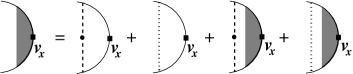
with

Figure 3: Full vertex including ladder and skew scattering diagrams.

III.3 Simple limits

III.3.1 Both subbands occupied

In the situation that both subbands are partially occupied, i.e., $\epsilon_{F}>h$, all contributions to the anomalous Hall conductivity vanish. For $\sigma_{yx}^{II}$ this is immediately evident from Eq. (23). For the skew scattering contribution, which is proportional to $\Gamma_{z}$ (see Eq. (36)), one observes easily that $\sigma_{yx}^{I(a),s}=0$ because $\Gamma_{z}=0$ (see Eq. (III.1)) due to $\nu_{+}/\lambda_{+}-\nu_{-}/\lambda_{-}=0$ (see Eq. (10)).

With respect to the bare bubble and ladder diagrams we will show in the following that they cancel mutually. For $\epsilon_{F}>h$ the integrals in Eq. (26) simplify to

$$I_{1}=\frac{\alpha^{2}m^{2}\epsilon_{F}}{2\lambda_{F}^{2}\Gamma}\,,\,\,\,\,I_{2}=-\frac{ihm}{2\lambda_{F}^{2}}\,,\,\,\,\,I_{3}=0\,,\,\,\,\,I_{4}=\frac{\alpha m}{2\Gamma}$$ (37)

and the bare momentum integrated vertices in Eq. (28) are:

$$n_{i}V_{0}^{2}\gamma_{x}=-\frac{\alpha h\Gamma}{\lambda_{F}^{2}}\,,\quad n_{i}V_{0}^{2}\gamma_{y}=\alpha\left(1-\frac{\alpha^{2}m\epsilon_{F}}{\lambda_{F}^{2}}\right)\,.$$ (38)

This gives for the bare bubble in Eq. (25)

$$\sigma_{yx}^{I(a),b}=-\frac{e^{2}}{2\pi}\frac{\alpha^{2}mh}{\lambda_{F}^{2}}\,.$$ (39)

For the ladder diagrams we need also

$$1-n_{i}V_{0}^{2}I_{1}=\frac{n_{i}V_{0}^{2}\gamma_{y}}{\alpha}\,,\quad-in_{i}V_{0}^{2}I_{2}=\frac{n_{i}V_{0}^{2}\gamma_{x}}{\alpha}$$ (40)

yielding

$$\sigma_{yx}^{I(a),l}\!\! = \!\!-\frac{e^{2}}{\pi}\frac{\alpha}{n_{i}V_{0}^{2}}\frac{2\gamma_{x}\gamma_{y}^{2}-\gamma_{x}\gamma_{y}^{2}+\gamma_{x}^{3}}{\gamma_{x}^{2}+\gamma_{y}^{2}}=-\frac{e^{2}}{\pi}\frac{\alpha\gamma_{x}}{n_{i}V_{0}^{2}}$$ (41)

$$= \frac{e^{2}}{2\pi}\frac{\alpha^{2}mh}{\lambda_{F}^{2}}$$

and thus

$$\sigma_{yx}^{I(a),b}+\sigma_{yx}^{I(a),l}=0\,,$$ (42)

i.e., the contribution of the bare bubble and the ladder diagrams cancel mutually.

III.3.2 Only majority band occupied

In the opposite situation, where only the majority band is partially occupied, we have $\nu_{+}=0$ and therefore $\Gamma_{z}\neq 0$. In this case all terms contribute to the anomalous Hall conductivity. In the following we restrict our analysis to Fermi energies $\epsilon_{F}>-h$, i.e., we disregard the region of very small Fermi energies, where the valley structure of the majority band becomes important (see Fig. 1(b)) and discuss the results in two simple limits: (i) small spin orbit interaction: $\alpha k_{F}\ll h$ and (ii) small magnetization $h\ll\alpha k_{F}$.

In the limit of small spin-orbit interaction $\alpha k_{F}\ll h$ the sum of bare bubble and ladder vertex corrections becomes

$$\sigma_{yx}^{I(a),b}+\sigma_{yx}^{I(a),l}=\frac{e^{2}}{2\pi}\frac{(\alpha k_{F})^{2}}{16h\epsilon_{F}}\left(3\frac{\epsilon_{F}}{h}+1\right)\left(-\frac{\epsilon_{F}}{h}+1\right)$$ (43)

the contribution from the states of the full Fermi sea

$$\sigma_{yx}^{II}=\frac{e^{2}}{4\pi}\frac{(\alpha k_{F})^{2}}{2h^{2}}$$ (44)

and the skew scattering term

$$\sigma_{yx}^{I(a),s}=\frac{e^{2}}{2\pi}\frac{(\alpha k_{F})^{2}}{8\epsilon_{F}n_{i}V_{0}}\frac{V_{1}^{3}}{V_{0}^{3}}\frac{(\epsilon_{F}+h)^{2}}{h^{2}}\,.$$ (45)

In the opposite limit of small exchange field $h\ll\alpha k_{F}$, considering first a spin-orbit interaction still smaller than the Fermi energy $\alpha k_{F}\ll\epsilon_{F}$, we find for the sum of bare bubble and ladder vertex corrections

$$\sigma_{yx}^{I(a),b}+\sigma_{yx}^{I(a),l}=-\frac{e^{2}}{2\pi}\frac{3h\epsilon_{F}}{(\alpha k_{F})^{2}}$$ (46)

and for the contribution from the states of the full Fermi sea

$$\sigma_{yx}^{II}=\frac{e^{2}}{4\pi}\left(1-\frac{h}{\alpha k_{F}}\right)$$ (47)

and for the skew scattering term

$$\sigma_{yx}^{I(a),s}=\frac{e^{2}}{2\pi}\frac{V_{1}^{3}}{V_{0}^{3}}\frac{2h\epsilon_{F}}{n_{i}V_{0}\alpha k_{F}}\,.$$ (48)

In the same limit where the exchange field is small $h\ll\alpha k_{F}$, but the spin-orbit interaction is now larger than the Fermi energy $\alpha k_{F}\gg\epsilon_{F}$ we find for the sum of bare bubble and ladder vertex corrections

$$\sigma_{yx}^{I(a),b}+\sigma_{yx}^{I(a),l}=-\frac{e^{2}}{2\pi}\frac{2h\epsilon_{F}^{3}}{(\alpha k_{F})^{4}}$$ (49)

and for the contribution from the states of the full Fermi sea

$$\sigma_{yx}^{II}=\frac{e^{2}}{4\pi}\left(1-\frac{2h\epsilon_{F}}{(\alpha k_{F})^{2}}\right)$$ (50)

and the for skew scattering term

$$\sigma_{yx}^{I(a),s}=\frac{e^{2}}{2\pi}\frac{V_{1}^{3}}{V_{0}^{3}}\frac{h}{n_{i}V_{0}}\,.$$ (51)

III.4 Discussion

We now discuss the full evaluation of the anomalous Hall conductivity in the limit of small spin orbit interaction $\alpha k_{F}\ll h$ and in the opposite limit of strong spin orbit interaction $\alpha k_{F}\gg h,\epsilon_{F}$. For the following discussion we will express all quantities in terms of the exchange field $h$, which we define as $h=1$. Furthermore we will set $m=1$, we choose $V_{1}=V_{0}$ and use an impurity concentration of $n_{i}=0.1$.

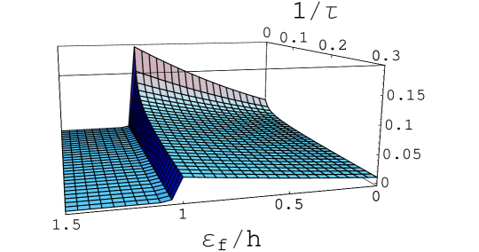
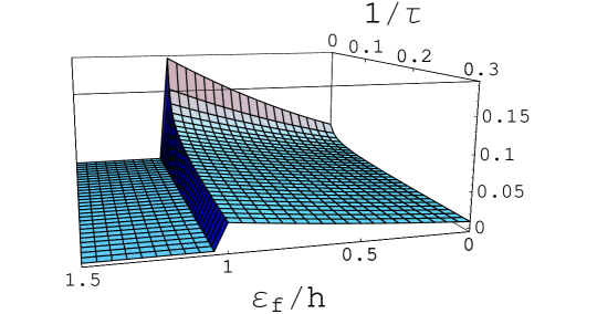
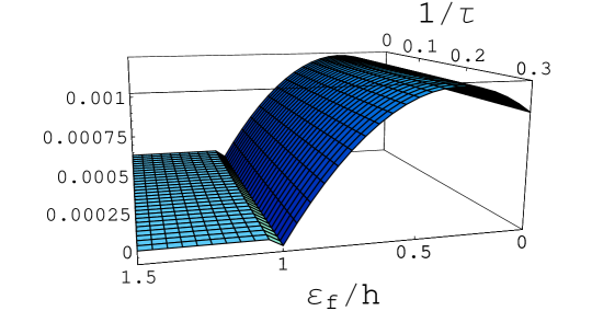
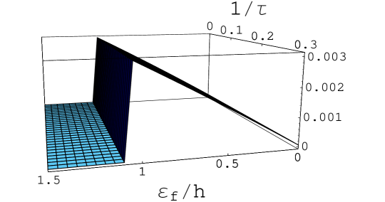
Figure 4: Anomalous Hall conductivity for $\alpha k_{F}/h=0.2$ and an impurity concentration of $n_{i}=0.1$ plotted as a function of $\epsilon_{F}/h$ (from right to left) and as a function of $1/\tau=n_{i}mV_{0}^{2}$ in units of $h$ (from back to front) where upper left panel: total anomalous Hall conductivity (Eq. (19)), upper right panel: skew scattering contribution (Eq. (36)), lower left panel: bare bubble plus ladder vertex corrections (Eq. (25)+Eq. (III.2.2)), lower right panel: $\sigma^{II}$ (Eq. (23)). All conductivities are plotted in units of $e^{2}$.

In Fig. 4 we show the anomalous Hall conductivity for a small spin orbit interaction of $\alpha k_{F}/h=0.2$ as a function of the Fermi energy $\epsilon_{F}/h$ and the scattering rate $1/\tau=n_{i}V_{0}^{2}m$ for an impurity concentration of $n_{i}=0.1$. The upper left panel shows the total anomalous Hall conductivity, i.e., the sum of skew scattering (upper right panel), of bare bubble and ladder diagrams (lower left panel) and of the contribution from the whole Fermi sea (lower right panel). Obviously all contributions to the total conductivity vanish for $\epsilon_{F}>h$, i.e., when both subbands are occupied which agrees with our analysis in Sec. III.3.1. Furthermore we observe that not only $\sigma_{yx}^{II}$ but also the bare bubble and ladder vertex corrections $\sigma_{yx}^{I(a),b}+\sigma_{yx}^{I(a),l}$ (see Eq. (43)) are independent of impurity scattering. Both contributions are small: $\sigma_{yx}^{II}$ contains a small prefactor of $(\alpha k_{F}/h)^{2}$ (see Eq. (44)) and $\sigma_{yx}^{I(a),b}+\sigma_{yx}^{I(a),l}$ a small prefactor of $(\alpha k_{F})^{2}/(h\epsilon_{F})$ (see Eq. (43)). The skew scattering contribution, on the other hand, has a prefactor of $\alpha k_{F}/(n_{i}V_{0})$ which diverges for $V_{0}\to 0$, i.e, $1/\tau\to 0$ (see Eq. (45)) and therefore overcompensates the small prefactor of $\alpha k_{F}/\epsilon_{F}$ (see Eq. (45)) when the impurity potentials $V_{0}$ becomes small enough. Thus for the parameters chosen in Fig. 4 the skew scattering term outweighs the other contributions by orders of magnitude and therefore the total anomalous Hall conductivity is almost identical to the skew scattering term. It increases quadratically with $\epsilon_{F}/h$ (see Eq. (45)) and then vanishes suddenly for $\epsilon_{F}>h$.

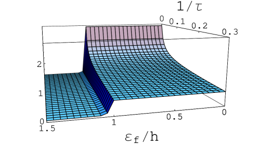
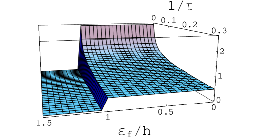
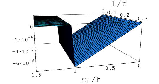
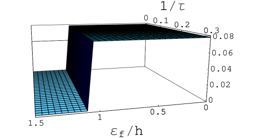
Figure 5: Anomalous Hall conductivity for $\alpha k_{F}/h=10.0$ and an impurity concentration of $n_{i}=0.1$ plotted as a function of $\epsilon_{F}/h$ (from right to left) and as a function of $1/\tau=n_{i}mV_{0}^{2}$ in units of $h$ (from back to front) where upper left panel: total anomalous Hall conductivity (Eq. (19)), upper right panel: skew scattering contribution (Eq. (36)), lower left panel: bare bubble plus ladder vertex corrections (Eq. (25)+Eq. (III.2.2)), lower right panel: $\sigma^{II}$ (Eq. (23)). All conductivities are plotted in units of $e^{2}$.

Fig. 5 displays the anomalous Hall conductivity in a similar way as Fig. 4 only for a large spin orbit interaction of $\alpha k_{F}/h=10$. Again, $\sigma_{yx}^{I(a),b}+\sigma_{yx}^{I(a),l}$ turns out to be independent of the impurity parameters and even smaller in magnitude as before because now it is suppressed by a small prefactor of $(h\epsilon_{F}^{3})/(\alpha k_{F})^{4}$ (see Eq. (49)). Analogously to the limit of small spin orbit interaction, the total anomalous Hall conductivity is dominated by the skew scattering contribution, which contains no small prefactor and due to the factor of $h/(n_{i}V_{0})$ grows rapidly for small impurity potentials $V_{0}\to 0$, i.e., $1/\tau\to 0$ (see Eq. (51)). In the limit of large spin-orbit interaction $\alpha k_{F}\gg\epsilon_{F}$ the skew scattering and thus the total anomalous Hall conductivity is independent of the Fermi energy $\epsilon_{F}$ for $\epsilon_{F}<h$ (see Eq. (51)) and then abruptly drops to zero for $\epsilon_{F}>h$.

IV Conclusions

In summary, we have investigated the anomalous Hall conductivity in a spin-polarized two-dimensional electron gas with Rashba spin-orbit interaction in the presence of pointlike potential impurities. Our calculations have been performed within diagrammatic perturbation theory based on the Kubo-Streda formula, an approach, which has previously been shown to yield equivalent results to the semiclassical Boltzmann treatment. Sinitsyn et al. (2006); Borunda:2007_a

Comparing our results with previous calculations we have been able to sort out contradictions existing in the literature. We have found that within the model Hamiltonian considered all contributions to the anomalous Hall conductivity vanish as soon as the minority band becomes partially filled, i.e., as soon as the Fermi energy becomes larger than the internal Zeeman field. For smaller Fermi energies all contributions are finite with $\sigma_{yx}^{II}$, the contribution from all states of the Fermi sea, being the smallest term at least in the limits of weak and of strong spin orbit interaction. The vertex corrections, which play the role of a side jump contribution, can be of similar magnitude as the intrinsic contribution and turn out to be independent of the impurity concentration and impurity potential at least in the limits of small and of strong spin orbit interaction. In the weak scattering limit the dominant contribution results from skew scattering because due to its $1/(n_{i}V_{0})$-dependence it outweighs all other terms. Moreover, the intrinsic and the side jump terms contain higher orders of small prefactors than the skew scattering contribution.

Appendix A Integration of $\sigma^{II}$

Starting from the expression of $\sigma^{II}$ in Eq. (20) one obtains after angular integration:

$$\sigma_{yx}^{II}=\frac{e^{2}}{4\pi}\frac{1}{2\pi}\!\!\int\!\!dkk\!\!\int_{-\infty}^{\infty}\!\!\!\!d\epsilon f(\epsilon)\frac{\alpha^{2}h}{\lambda_{k}}4{\rm Im}\left[G_{+}^{R}G_{-}^{R}(G_{-}^{R}-G_{+}^{R})\right].$$ (52)

Now performing the remaining integrals in the clean limit, i.e., using $\Gamma_{+}=\Gamma_{-}=\delta$, yields

$$\sigma_{yx}^{II} = \frac{e^{2}}{4\pi}\frac{1}{2\pi}\int dkk\int_{-\infty}^{\infty}d\epsilon f(\epsilon)4\frac{\alpha^{2}h}{\lambda_{k}}(E_{k-}-E_{k+})$$

$${\rm Im}\left[\frac{1}{(\epsilon-E_{k+}+i\delta)^{2}(\epsilon-E_{k-}+i\delta)^{2}}\right]$$

$$= \frac{e^{2}}{4\pi}\frac{1}{2\pi}\int dkk4\frac{\alpha^{2}h}{\lambda_{k}}\frac{1}{E_{k-}-E_{k+}}$$

$$\bigl{\{}\pi\delta(E_{k+}-\epsilon_{F})+\pi\delta(E_{k-}-\epsilon_{F})$$

$$-\frac{2}{E_{k+}-E_{k-}}{\rm Im}\left[\ln(E_{k+}-\epsilon_{F}-i\delta)\right.$$

$$\left.\hskip 62.59596pt-\ln(E_{k-}-\epsilon_{F}-i\delta)\right]\bigr{\}}.$$

Substituting $E_{k+}-E_{k-}=2\lambda_{k}$ and using

$$\int dk\frac{k}{\lambda_{k}^{2}}\pi\delta(E_{k\pm}-\epsilon_{F})$$

$$=\int_{\pm h}^{\infty}dE_{k\pm}\frac{m}{\lambda_{k}|\lambda_{k}\pm\alpha^{2}m|}\pi\delta(E_{k\pm}-\epsilon_{F})$$

$$=\frac{\pi m}{\lambda_{\pm}|\lambda_{\pm}\pm\alpha^{2}m|}\Theta(\epsilon_{F}-E_{\pm}^{\rm min})$$ (54)

and

$$\int dk\frac{k}{\lambda_{k}^{3}}\ln(E_{k\pm}-\epsilon_{F}-i\delta)=\left[-\frac{\ln(E_{k\pm}-\epsilon_{F}-i\delta)}{\alpha^{2}\lambda_{k}}\right]_{0}^{\infty}$$

$$+\int_{0}^{\infty}\frac{dk}{\alpha^{2}\lambda_{k}}\frac{1}{E_{k\pm}-\epsilon_{F}-i\delta}\frac{dE_{k\pm}}{dk}$$ (55)

and

$$-\left[-\frac{\ln(E_{k+}-\epsilon_{F}-i\delta)}{\alpha^{2}\lambda_{k}}\right]_{0}^{\infty}+\left[-\frac{\ln(E_{k-}-\epsilon_{F}-i\delta)}{\alpha^{2}\lambda_{k}}\right]_{0}^{\infty}$$

$$=-\frac{i\pi}{\alpha^{2}h}\Theta(h-\epsilon_{F})$$ (56)

$\sigma^{II}$ simplifies to

$$\sigma_{yx}^{II} = -\frac{e^{2}}{4\pi}h\left(\frac{1}{m}\frac{1}{\lambda_{-}-\alpha^{2}m}-\frac{1}{m}\frac{1}{\lambda_{+}+\alpha^{2}m}\Theta(\epsilon_{F}-h)\right.$$

$$\left.\qquad\qquad-\frac{1}{h}\Theta(h-\epsilon_{F})\right)$$

$$= \frac{e^{2}}{4\pi}\left(1-\frac{h}{\sqrt{h^{2}+2\alpha^{2}m\epsilon_{F}+(\alpha^{2}m)^{2}}}\right)\Theta(h-\epsilon_{F}).$$

Appendix B Integrals in the weak scattering limit

In the weak scattering limit ($\Gamma,\Gamma_{z}$ small) the integrals over two Greens functions simplify to:

$$\frac{1}{2\pi}\int dkkf(k)G_{+}^{R}(k)G_{+}^{A}(k)$$ (58)

$$=\frac{1}{2\pi}\int dkkf(k)\frac{1}{\epsilon_{F}-E_{k+}+i\Gamma_{+}}\frac{1}{\epsilon_{F}-E_{k+}-i\Gamma_{+}}$$

$$=\frac{1}{2\pi}\int dE_{k+}\nu_{+}f(k(E_{k+}))\frac{1}{\Gamma_{+}}\frac{\Gamma_{+}}{(E_{k+}^{2}-\epsilon_{F}^{2})^{2}+\Gamma_{+}^{2}}$$

$$\approx\frac{\nu_{+}f(k_{+})}{2\Gamma_{+}}$$

$$\frac{1}{2\pi}\int dkkf(k)G_{-}^{R}(k)G_{-}^{A}(k)\approx\frac{\nu_{-}f(k_{-})}{2\Gamma_{-}}\,\,\,{\rm analogously}$$

and

$$\frac{1}{2\pi}\int dkkf(k)G_{+}^{R}(k)G_{-}^{A}(k)$$ (59)

$$=\frac{1}{2\pi}\int dkkf(k)\frac{1}{\epsilon_{F}-E_{k+}+i\Gamma_{+}}\frac{1}{\epsilon_{F}-E_{k-}-i\Gamma_{-}}$$

$$\approx\frac{1}{2\pi}\int dkkf(k)\left(\frac{1}{\epsilon_{F}-E_{k+}}-i\pi\delta(\epsilon_{F}-E_{k+})\right)$$

$$\hskip 73.97733pt\left(\frac{1}{\epsilon_{F}-E_{k-}}+i\pi\delta(\epsilon_{F}-E_{k-})\right)$$

$$\approx\frac{1}{2\pi}\int dkkf(k)\frac{1}{\epsilon_{F}-\epsilon_{k}-\lambda_{k}}\frac{1}{\epsilon_{F}-\epsilon_{k}+\lambda_{k}}$$

$$+\frac{i}{2}\int dkkf(k)\left(\delta(\epsilon_{F}-\epsilon_{k}+\lambda_{k})\frac{1}{\epsilon_{F}-\epsilon_{k}-\lambda_{k}}\right.$$

$$\left.\hskip 65.44142pt-\delta(\epsilon_{F}-\epsilon_{k}-\lambda_{k})\frac{1}{\epsilon_{F}-\epsilon_{k}+\lambda_{k}}\right)$$

yielding

$$\frac{1}{2\pi}\int dkkf(k)(G_{+}^{R}(k)G_{-}^{A}(k)-G_{-}^{R}(k)G_{+}^{A}(k))$$

$$\approx i\int dE_{k-}\frac{\nu_{-}f(k(E_{k-}))\delta(\epsilon_{F}-E_{k-})}{\epsilon_{F}-E_{k-}-2\lambda_{k(E_{k-})}}$$

$$-i\int dE_{k+}\frac{\nu_{+}f(k(E_{k+}))\delta(\epsilon_{F}-E_{k+})}{\epsilon_{F}-E_{k+}+2\lambda_{k(E_{k+})}}$$

$$=-\frac{i}{2}\left(\frac{\nu_{+}f(k_{+})}{\lambda_{+}}+\frac{\nu_{-}f(k_{-})}{\lambda_{-}}\right).$$ (60)

Now we find for the integrals $I_{1}$, $I_{2}$, $I_{3}$ and $I_{4}$ in the weak scattering limit:

$$I_{1}\!\! = \!\!\frac{1}{2\pi}\int dkk\left(G_{0}^{R}G_{0}^{A}-G_{z}^{R}G_{z}^{A}\right)$$

$$= \!\!\frac{1}{4}\frac{1}{2\pi}\int dkk\left(G_{+}^{R}G_{+}^{A}+G_{-}^{R}G_{-}^{A}+G_{+}^{R}G_{-}^{A}+G_{-}^{R}G_{+}^{A}\right.$$

$$\!\!\!\!\!\!\left.-\frac{\lambda_{k}^{2}(h^{2}+\Gamma_{z}^{2})}{\lambda_{k}^{4}+h^{2}\Gamma_{z}^{2}}\left(G_{+}^{R}G_{+}^{A}+G_{-}^{R}G_{-}^{A}-G_{+}^{R}G_{-}^{A}-G_{-}^{R}G_{+}^{A}\right)\!\right)$$

$$\approx \frac{1}{4}\frac{1}{2\pi}\int dkk\left(1-\frac{h^{2}}{\lambda_{k}^{2}}\right)\left(G_{+}^{R}G_{+}^{A}+G_{-}^{R}G_{-}^{A}\right)$$

$$\approx \frac{1}{8}\left(\left(1-\frac{h^{2}}{\lambda_{+}^{2}}\right)\frac{\nu_{+}}{\Gamma_{+}}+\left(1-\frac{h^{2}}{\lambda_{-}^{2}}\right)\frac{\nu_{-}}{\Gamma_{-}}\right)$$

$$I_{2}\!\! = \!\!\!\frac{1}{2\pi}\int dkk\left(G_{0}^{R}G_{z}^{A}-G_{z}^{R}G_{0}^{A}\right)$$

$$= \!\!\!-\frac{1}{2}\frac{1}{2\pi}\int\!\!dkk\frac{\lambda_{k}}{\lambda_{k}^{4}+\Gamma_{z}^{2}h^{2}}\left(h(\lambda_{k}^{2}\!+\!\Gamma_{z}^{2})(G_{-}^{R}G_{+}^{A}\!-\!G_{+}^{R}G_{-}^{A})\right.$$

$$\hskip 79.6678pt+\left.i\Gamma_{z}(h^{2}\!-\!\lambda_{k}^{2})(G_{+}^{R}G_{+}^{A}\!-\!G_{-}^{R}G_{-}^{A})\right)$$

$$\approx \!\!\!-\frac{1}{2}\frac{1}{2\pi}\int\!\!dkk\frac{1}{\lambda_{k}^{3}}\left(h\lambda_{k}^{2}(-G_{+}^{R}G_{-}^{A}+G_{-}^{R}G_{+}^{A})\right.$$

$$\hskip 59.75095pt\left.+i\Gamma_{z}(h^{2}-\lambda_{k}^{2})(G_{+}^{R}G_{+}^{A}-G_{-}^{R}G_{-}^{A})\right)$$

$$\approx \!\!\!-\frac{i}{4}\!\left(\!\frac{\nu_{+}h}{\lambda_{+}^{2}}\!+\!\frac{\nu_{-}h}{\lambda_{-}^{2}}\!+\!\frac{\Gamma_{z}}{\Gamma_{+}}\frac{\nu_{+}(h^{2}\!-\!\lambda_{+}^{2})}{\lambda_{+}^{3}}\!-\!\frac{\Gamma_{z}}{\Gamma_{-}}\frac{\nu_{-}(h^{2}\!-\!\lambda_{-}^{2})}{\lambda_{-}^{3}}\!\right)$$

$$I_{3}\!\! = \!\!\frac{1}{2\pi}\int dk\frac{k^{2}}{2m}\left(\tilde{G}_{y}^{R}G_{z}^{A}-G_{z}^{R}\tilde{G}_{y}^{A}\right)$$

$$= \!\!-\frac{i}{2}\frac{1}{2\pi}\int dkk\frac{k^{2}}{2m}\frac{\alpha\Gamma_{z}\lambda_{k}^{2}}{\lambda_{k}^{4}+\Gamma_{z}^{2}h^{2}}(G_{+}^{R}G_{+}^{A}+G_{-}^{R}G_{-}^{A}$$

$$\hskip 119.50148pt-G_{+}^{R}G_{-}^{A}-G_{-}^{R}G_{+}^{A})$$

$$\approx \!\!-\frac{i}{2}\frac{1}{2\pi}\int dkk\frac{k^{2}}{2m}\frac{\alpha\Gamma_{z}}{\lambda_{k}^{2}}(G_{+}^{R}G_{+}^{A}+G_{-}^{R}G_{-}^{A})$$

$$\approx \!\!-\frac{i}{4}\alpha\Gamma_{z}\left(\epsilon_{F}\left(\frac{\nu_{+}}{\Gamma_{+}\lambda_{+}^{2}}+\frac{\nu_{-}}{\Gamma_{-}\lambda_{-}^{2}}\right)-\frac{\nu_{+}}{\Gamma_{+}\lambda_{+}}+\frac{\nu_{-}}{\Gamma_{-}\lambda_{-}}\right)$$

$$I_{4}\!\! = \!\!\frac{1}{2\pi}\int dk\frac{k^{2}}{2m}\left(G_{0}^{R}\tilde{G}_{y}^{A}+\tilde{G}_{y}^{R}G_{0}^{A}\right)$$

$$= \!\!-\frac{1}{2}\frac{1}{2\pi}\int dkk\frac{k^{2}}{2m}\frac{\alpha\lambda_{k}}{\lambda_{k}^{4}+\Gamma_{z}^{2}h^{2}}\left(\lambda_{k}^{2}(G_{+}^{R}G_{+}^{A}-G_{-}^{R}G_{-}^{A})\right.$$

$$\hskip 108.12054pt\left.+i\Gamma_{z}h(G_{-}^{R}G_{+}^{A}-G_{+}^{R}G_{-}^{A})\right)$$

$$\approx \!\!-\frac{1}{2}\frac{1}{2\pi}\int dkk\frac{k^{2}}{2m}\frac{\alpha}{\lambda_{k}}(G_{+}^{R}G_{+}^{A}-G_{-}^{R}G_{-}^{A})$$

$$\approx \!\!-\frac{1}{4}\alpha\left(\epsilon_{F}\left(\frac{\nu_{+}}{\Gamma_{+}\lambda_{+}}-\frac{\nu_{-}}{\Gamma_{-}\lambda_{-}}\right)-\left(\frac{\nu_{+}}{\Gamma_{+}}+\frac{\nu_{-}}{\Gamma_{-}}\right)\right).$$

References

(1) E. H. Hall, Philos. Mag. 10, 301 (1880);
Philos. Mag. 12, 157 (1881).
Sinova et al. (2004)
J. Sinova,
T. Jungwirth, and
J. Cerne,
Int. J. Mod. Phys. B 18,
1083 (2004).
Karplus and Luttinger (1954)
R. Karplus and
J. M. Luttinger,
Phys. Rev. 95,
1154 (1954).
Smit (1955)
J. Smit,
Physica 21,
877 (1955).
(5) Note that the origin of the asymmetry of this scattering arises from the spin-orbit coupling present in the Bloch states and not from the very weak spin-orbit coupling contribution of the disorder potential as noted originally by Smit. When projecting a multi-band system to an effective conduction band system one can obtain a term that looks as if it arises from such a spin-orbit coupling part of the disorder potential but it truly originates from spin-orbit coupling induced by the valence band states and the normal disorder that is felt by them.
Berger (1970)
L. Berger,
Phys. Rev. B 2,
4559 (1970).
Nozieres and Lewiner (1973)
P. Nozieres and
C. Lewiner,
Le Journal de Physique 34,
901 (1973).
Kohn and Luttinger (1957)
W. Kohn and
J. M. Luttinger,
Phys. Rev. 108,
590 (1957).
Luttinger (1958)
J. M. Luttinger,
Phys. Rev. 112,
739 (1958).
Sinitsyn et al. (2006)
N. A. Sinitsyn,
A. H. MacDonald,
T. Jungwirth,
V. K. Dugaev,
and J. Sinova
Phys. Rev. B 75, 045315 (2007).
Culcer (2003)
D. Culcer,
A. H. MacDonald, and
Q. Niu,
Phys. Rev. B 68,
045327 (2003).
Dugaev et al. (2005)
V. K. Dugaev,
P. Bruno,
M. Taillefumier,
B. Canals, and
C. Lacroix,
Phys. Rev. B 71,
224423 (2005).
Sinitsyn et al. (2005)
N. A. Sinitsyn,
Q. Niu,
J. Sinova, and
K. Nomura,
Phys. Rev. B 72,
045346 (2005).
Liu and Lei (2005)
S. Y. Liu and
X. L. Lei,
Phys. Rev. B 72,
195329 (2005).
Liu and Lei (2005)
S. Y. Liu,
N. J. M. Horing, and
X. L. Lei,
Phys. Rev. B 74,
165316 (2006).
ichiro Inoue et al. (2006)
J. Inoue,
T. Kato,
Y. Ishikawa,
H. Itoh,
G. E. W. Bauer,
and L. W.
Molenkamp,
Phys. Rev. Lett.
97, 046604
(2006).
Onoda et al. (2006)
S. Onoda,
N. Sugimoto, and
N. Nagaosa,
Phys. Rev. Lett. 97, 126602 (2006).
(18) M. F. Borunda, T. S. Nunner, T. Luck,
N. A. Sinitsyn, C. Timm, J. Wunderlichl, T. Jungwirth, A. H. MacDonald, and J. Sinova,
cond-mat/0702289 (2007).
(19) N. A. Sinitsyn, Q. Niu, and A. H. MacDonald
Phys. Rev. B 73, 075318 (2006).
Streda (1982)
P. Streda,
J. Phys.
C 15, L717 (1982).