On the width of cold fronts in clusters of galaxies due to conduction

Abstract

We consider the impact of thermal conduction in clusters of galaxies on the (unmagnetized) interface between a cold gaseous cloud and a hotter gas flowing over the cloud (the so-called cold front). We argue that near the stagnation point of the flow conduction creates a spatially extended layer of constant thickness $\Delta$, where $\Delta$ is of order $\sim\sqrt{kR/U}$, and $R$ is the curvature radius of the cloud, $U$ is the velocity of the flow at infinity, and $k$ is the conductivity of the gas. For typical parameters of the observed fronts, one finds $\Delta\ll R$. The formation time of such a layer is $\sim R/U$. Once the layer is formed, its thickness only slowly varies with time and the quasi-steady layer may persist for many characteristic time scales. Based on these simple arguments one can use the observed width of the cold fronts in galaxy clusters to constrain the effective thermal conductivity of the intra-cluster medium.

1 Introduction

Chandra observations of galaxy clusters often show sharp discontinuities in the surface brightness of the hot intra-cluster medium (ICM) emission (Markevitch et al., 2000, Vikhlinin, Markevitch, Murray, 2001, see Markevitch & Vikhlinin 2007 for a review). Most of these structures have lower temperature gas on the brighter (higher density) side of the discontinuity, contrary to the expectation for non-radiative shocks in the ICM. Within the measurement uncertainties, the pressure is continuous across these structures, suggesting that they are contact discontinuities rather than shocks. In the literature these structures are now called “cold fronts”.

There are several plausible mechanisms responsible for the formation of such cold fronts, all of them involving relative motion of the cold and hot gases. Below we will consider the case of a hot gas flow over a colder gravitationally bound gas cloud, which is a prototypical model of a cold front. In such a situation one expects that ram pressure of the hotter gas strips the outer layers of the colder cloud, exposing denser gas layers and forming a cold front near the stagnation point of the hot flow (Markevitch et al., 2000, Vikhlinin et al., 2001a, Bialek, Evrard and Mohr, 2002, Nagai & Kravtsov, 2003, Acreman et al., 2003, Heinz et al., 2003, Asai, Fukuda & Matsumoto, 2004, 2007, Mathis et al., 2005, Tittley & Henriksen, 2005, Takizawa, 2005, Ascasibar & Markevitch 2006) .

Some of the observed cold fronts are remarkably thin. For example, the width of the front in Abell 3667 (Vikhlinin et al., 2001a) is less than $5\,{\rm kpc}$, which is comparable to the electron mean free path. Given that the temperature changes across the front by a factor of $\sim 2$, thermal conduction (if not suppressed) should strongly affect the structure of the front (e.g. Ettori & Fabian, 2000). In fact, suppression of conduction by magnetic fields is likely to happen along the cold front since gas motions on both sides of the interface may produce preferentially tangential magnetic field, effectively shutting down the heat flux across the front (e.g. Vikhlinin et al., 2001b, Narayan & Medvedev, 2001, Asai et al., 2004, 2005, 2007, Lyutikov 2006). While magnetic fields are hence likely to play an important role in shaping cold fronts, it is still interesting to consider the expected structure of a cold front in the idealized case of an unmagnetized plasma.

The structure of this paper is as follows. In Section 2, basic equations are listed and a toy model of a thermally broadened interface between cool and hot gas is discussed. In Section 3, we present the results of numerical simulations of hot gas flowing past a cooler gas cloud. In Section 4, we discuss how limits on the effective conductivity can be obtained for the observed cold fronts. Finally, we summarize our findings in Section 5.

2 Thermal conduction near the stagnation point of the flow

2.1 Basic equations

We parameterize the isotropic thermal conductivity $k$ as

$$k=f\times k_{0},$$ (1)

where $f<1$ is the suppression coefficient of the conductivity relative to the conductivity $k_{0}$ of an unmagnetized plasma (Spitzer 1962, Braginskii 1965):

$$k_{0}=4.6\times 10^{13}\left(\frac{T}{10^{8}\,{\rm K}}\right)^{5/2}\left(\frac{\rm{ln}\Lambda}{40}\right)^{-1}{\rm erg~{}cm^{-1}~{}s^{-1}~{}K^{-1}},$$ (2)

where $T$ is the gas temperature, and $\rm{ln}\Lambda$ is the Coulomb logarithm.

If the scale length of temperature gradients is much larger than the particle mean free path, then saturation of the heat flux (Cowie & McKee, 1977) can be neglected and the evolution of the temperature distribution can be obtained by solving the mass, momentum and energy conservation equations with the heat diffusion term ${\mn@boldsymbol{\nabla}}\cdot k{\mn@boldsymbol{\nabla}}T$ in the energy equation (e.g. Landau & Lifshitz, 1959):

$$\frac{\partial\rho}{\partial t}+{\mn@boldsymbol{\nabla}}\cdot(\rho{{\mn@boldsymbol{v}}})=0,$$ (3)

$$\frac{\partial{{\mn@boldsymbol{v}}}}{\partial t}+\left({{\mn@boldsymbol{v}}}\cdot{\mn@boldsymbol{\nabla}}\right){{\mn@boldsymbol{v}}}=-\frac{1}{\rho}{\mn@boldsymbol{\nabla}}p+g,$$ (4)

$$\frac{\partial}{\partial t}\left(\frac{\rho{{\mn@boldsymbol{v}}}^{2}}{2}+\rho\epsilon\right)={\mn@boldsymbol{\nabla}}\cdot k{\mn@boldsymbol{\nabla}}T-{\mn@boldsymbol{\nabla}}\cdot\rho{\rm v}\left(\frac{{{\mn@boldsymbol{v}}}^{2}}{2}+\omega\right),$$ (5)

where $\rho$ is the gas density, $p$ is the gas pressure, $g$ is the gravitational acceleration, and $v$ is the gas velocity. We adopt an ideal gas with $\gamma=5/3$, where $\epsilon=\frac{1}{\gamma-1}\frac{k_{B}T}{\mu m_{p}}$, $\omega=\frac{\gamma}{\gamma-1}\frac{k_{B}T}{\mu m_{p}}$, and $p=\frac{\rho}{\mu m_{p}}k_{B}T$.

In the next section we first consider the simplified case of passive scalar diffusion in a time independent velocity flow, while in Section 3 we discuss numerical solutions of the above equations.

2.2 Toy model

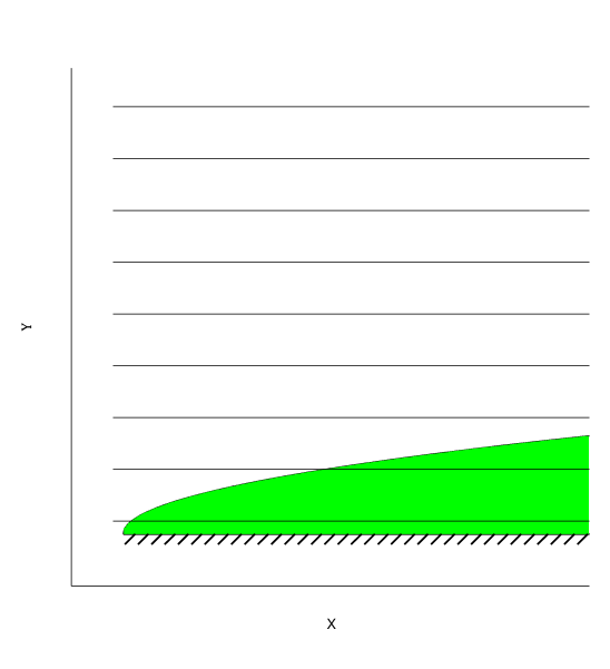
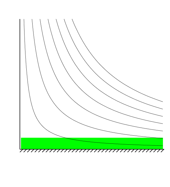
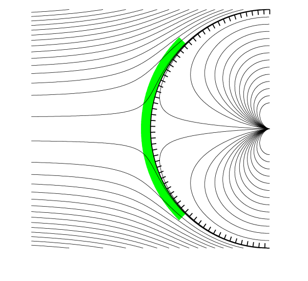
Figure 1: Examples of simple potential flows: uniform flow past a plate (left), flow into a 90 degree corner (middle) and flow past a sphere (right). Streamlines are shown as thin solid lines. The shaded areas schematically indicate the width of the layer formed by diffusion.

Churazov & Inogamov (2004) noted that the behaviour of a conducting layer in cold fronts should be similar to the behaviour of a viscous layer near a plate or near the surface of a blunt body (see e.g. Batchelor, 1967). When the fluid is advected along the surface, the thickness of the layer grows in proportion to the square root of the advection time. Near the stagnation point, the velocity of the flow increases linearly with the distance from the stagnation point and the characteristic advection time is approximately constant. Therefore the thickness of the layer can also be approximately constant. Below we provide a more rigorous justification of this picture.

Let us consider the simple case of diffusion of a passive scalar $\psi$ in a potential flow of an incompressible fluid. The diffusion coefficient $D$ is assumed to be constant and the velocity field is known and constant with time. The diffusion equation

$$\frac{\partial\psi}{\partial t}+{\mn@boldsymbol{\nabla}}\cdot({{\mn@boldsymbol{v}}}\psi)-D\Delta\psi=0$$ (6)

is supplemented by static boundary conditions at the surface of the body and at large distance from the body. For a steady state solution ($\frac{\partial\psi}{\partial t}=0$) and for an incompressible fluid (${\mn@boldsymbol{\nabla}}\cdot{\mn@boldsymbol{v}}=0$) the above equation reduces to

$${{\mn@boldsymbol{v}}}\cdot{\mn@boldsymbol{\nabla}}\psi-D\Delta\psi=0.$$ (7)

In the simplest case of a uniform flow along the “heated” plate (Fig. 1 left), ${v_{x}}=u={\rm const}$ and ${v}_{y}=0$. At sufficiently large distance from the leading edge of the plate, the derivative $\frac{\partial^{2}\psi}{\partial^{2}x}$ can be neglected and equation (7) can be written as

$$u\frac{\partial\psi}{\partial x}-D\frac{\partial^{2}\psi}{\partial y^{2}}=0.$$ (8)

An obvious solution in the form $\psi=f(y/\sqrt{x})$ is given by

$$\psi=(\psi_{1}-\psi_{2})~{}{\rm Erf}\left(\sqrt{\frac{u}{2Dx}}y\right)+\psi_{2},$$ (9)

where $\psi_{2}$ and $\psi_{1}$ are the values of the scalar at the plate and at infinity, respectively. The width of the interface is therefore $\Delta y=\sqrt{\frac{2D}{u}x}$ and it increases with the distance $x$ from the leading edge of the plate as $\sqrt{x}$. Since it takes a time $t=x/u$ for the gas to flow from the edge of the plate to a given position $x$, the width of the diffusive layer is simply $\sim\sqrt{Dt}=\sqrt{Dx/u}$.

Consider now a potential flow into a 90 degrees corner (Fig. 1 middle), governed by the velocity potential $\phi=Ar^{2}\cos{2\theta}$ (see e.g. Lamb 1932, for various examples of potential flows). Here $r$ is the distance from the corner and $\theta$ is angle from the horizontal axis. In this case the velocity components are ${v}_{x}=2Ax$ and ${v}_{y}=-2Ay$. An obvious solution to equation (7) is then

$$\psi=(\psi_{1}-\psi_{2})~{}{\rm Erf}\left(\sqrt{\frac{A}{D}}y\right)+\psi_{2},$$ (10)

with the width $y=\sqrt{\frac{D}{A}}$ of the interface being independent of $x$. The reason for this behaviour is clear: the acceleration of the (incompressible) fluid along the interface causes a contraction of the fluid elements perpendicular to the direction of the acceleration. While diffusion is trying to make the interface broader, the motion of the fluid towards the interface compensates for the broadening of the interface, and a steady state is reached (Fig. 1 middle).

The potential flow past a cylinder or sphere behaves qualitatively similar (Fig. 1 right). Indeed, in the vicinity of the stagnation point (for $\theta\ll 1$), the radial and tangential components can be written as (flow is from the right to the left, angle is counted clockwise from the $-x$ direction):

$${v}_{r}=-U\left(1-\frac{R^{2}}{r^{2}}\right)\cos{\theta}\approx-2U\frac{\eta}{R}$$

$${v}_{\theta}=U\left(1+\frac{R^{2}}{r^{2}}\right)\sin{\theta}\approx 2U\frac{\zeta}{R},$$ (11)

for a cylinder and

$${v}_{r}=-U\left(1-\frac{R^{3}}{r^{3}}\right)\cos{\theta}\approx-3U\frac{\eta}{R}$$

$${v}_{\theta}=U\left(1+\frac{R^{3}}{2r^{3}}\right)\sin{\theta}\approx\frac{3}{2}U\frac{\zeta}{R}$$ (12)

for a sphere. Here $U$ is the velocity at infinity, $R$ is the radius of the cylinder or sphere, $\eta=r-R$ and $\zeta=R\sin{\theta}$.

In the same approximation as for the cases discussed above (where the spatial derivative of $\psi$ along $\zeta$ is neglected) the diffusion equation reduces to

$$-v_{r}\frac{\partial\psi}{\partial r}-D\frac{\partial^{2}\psi}{\partial r^{2}}=0,$$ (13)

and the width of the interface over the radius is set by the diffusion coefficient $D$ and the coefficient $C$ in the relation $v_{r}=-C\eta$, yielding

$$\Delta r\approx\sqrt{\frac{2D}{C}}=\left\{\begin{array}[]{ll}\sqrt{D\frac{R}{U}}&{\rm cylinder}\\ &\\ \sqrt{\frac{2}{3}D\frac{R}{U}}&{\rm sphere.}\end{array}\right.$$ (17)

In this case the width of the interface is also constant along the surface of the cylinder or sphere (Fig. 1 right).

One can also consider a closer analogue of a flow past a spherical cloud by extending the solution for a potential flow into the inner part of the cylinder or sphere, as illustrated in Fig. 1. In this model there is a circulation flow of gas inside the cloud, and the tangential component of the velocity is continuous across the boundary while the normal component is zero at the boundary. We can further allow for different densities $\rho_{1}$ and $\rho_{2}$ outside and inside of the boundary if all velocities inside are scaled by a factor $\sqrt{\rho_{1}/\rho_{2}}$. The resulting configuration can be considered as an idealized (and unstable) analogue of a hot flow past a colder cloud in the absence of gravity (see also Heinz et al., 2003). Allowing different diffusion coefficients $D_{1}$ and $D_{2}$ in the flow outside and inside the boundary, and requiring the solution $\psi$ and its spatial derivative to be continuous across the interface, yields the following solution in the vicinity of the stagnation point:

$$\psi = (\psi_{1}-\psi_{m})~{}{\rm Erf}\left(\sqrt{\frac{C_{1}}{2D_{1}}}(r-r_{0})\right)+\psi_{m}\;\;{\rm outside,}$$

$$\psi = (\psi_{m}-\psi_{2})~{}{\rm Erf}\left(\sqrt{\frac{C_{2}}{2D_{2}}}(r-r_{0})\right)+\psi_{m},\;\;{\rm inside}$$

$$\psi_{m} = \frac{\psi_{1}+\psi_{2}\frac{D_{2}}{D_{1}}\frac{C_{1}}{C_{2}}}{1+\frac{D_{2}}{D_{1}}\frac{C_{1}}{C_{2}}}.$$

Here $r_{0}$ is the radius of the boundary, $\psi_{1}$ and $\psi_{2}$ are the values far from the interface, $C_{2}=C_{1}\sqrt{\rho_{1}/\rho_{2}}$, and $C_{1}=2U/R$ for a cylinder or $C_{1}=3U/R$ for a sphere, respectively. The width of the interface is again constant along the boundary.

The same answer is obviously valid for any idealized flow of this type: near the stagnation point the width of the “heated” layer does not change along the surface of the body. Real cold fronts are of course much more complicated structures. However, the acceleration of the flow along the interface and the simultaneous contraction in the perpendicular direction are generically present also here. It can therefore be expected that the width of the interface will be similarly constant in real cold fronts. A simple extension of the above toy model can be obtained by allowing for gas compressibility and a temperature dependent conductivity, i.e. by considering the full system of equations (3)-(5) with conductivity according to eq. (2). An expansion of heated layers and simultaneous contraction of cooled layers on the other side of the interface will certainly modify the flow, but for the transonic flows of interest here we might expect that the results obtained for a toy model will still be approximately valid. In the next section we verify this prediction using numerical simulations.

3 Numerical simulations

For our numerical experiments, we used the TreeSPH code GADGET-2 (Springel, 2005) combined with the implementation of thermal conduction discussed by Jubelgas, Springel & Dolag (2004), which accounts both for the saturated and unsaturated regimes of the heat flux.

The simulations were intended to illustrate a simple toy model, described in section 2.2, rather than to provide a realistic description of the observed cold fronts. The specific goal was to see the impact of the flow stretching near the stagnation point on the width of the interface set by conduction. With this in mind we intentionally restricted ourselves to a 2D geometry and an unmagnetized plasma. For a 3D calculation of magnetized clouds see Asai et al. (2007). The self gravity of gas particles was also neglected in our idealized simulations and all gas motions were happening in a static gravitational potential. Given that the typical gas mass fraction in clusters is of order 10-15 per cent, the self gravity of gas particles is likely to be a second order effect. A more significant simplification is the assumption of a static potential, since at least some of the cold fronts are caused by cluster mergers where strong changes of the potential are possible. Formation of cold fronts in the appropriate cosmological conditions was considered by e.g. Bialek et al. (2002), Nagai & Kravtsov (2003), Mathis et al. (2005), see also Tittley & Henriksen (2005) and Ascasibar & Markevitch (2006). Our illustrative 2D simulations, described below, can be viewed as a “minimal” configuration which allows us to see the effect of flow stretching and to extend the toy model to the case of a compressible gas and a temperature dependent diffusion coefficient.

3.1 Initial conditions

Our 2D simulations of cold fronts in clusters were carried out in a 8x4 Mpc periodic box. We represented the cluster with a static King gravitational potential of the form

$$\phi=-9\sigma^{2}\frac{\ln{\left[x+\sqrt{1+x^{2}}\right]}}{x},$$ (18)

with $\sigma=810\,{\rm km\,s^{-1}}$, $x=r/r_{c}$ and $r_{c}=300$ kpc. The initial temperature and density distributions were set to

$$(T_{e},\rho)=\left\{\begin{array}[]{ll}(T_{1},\frac{\rho_{1}}{(1+x^{2})^{\frac{3}{2}}})&x<x_{\rm out}\\ &\\ (T_{2},\frac{\rho_{2}}{(1+x^{2})^{\frac{3}{2}\frac{T_{1}}{T_{2}}}})&x>x_{\rm out}\end{array}\right.$$ (22)

where

$$\rho_{2}=\frac{\rho_{1}}{(1+x_{\rm out}^{2})^{\frac{3}{2}}}\frac{T_{1}}{T_{2}}\left[(1+x_{\rm out}^{2})^{\frac{3}{2}}\frac{T_{1}}{T_{2}}\right],$$ (23)

and $kT_{1}=\mu m_{p}\sigma^{2}\approx 4$ keV. Thus the temperature and density make a jump at $x_{\rm out}$, while the pressure is continuous. In our runs, $T_{2}=8$ keV, $x_{\rm out}=1$, $\mu=0.61$, and $\rho_{1}=6.6\times 10^{-26}~{}{\rm g~{}cm^{-3}}$. The gas velocity was set to zero for $x<x_{\rm out}$ and to $u=2000~{}{\rm km~{}s^{-1}}$ for $x>x_{\rm out}$. The corresponding Mach number relative to the hot 8 keV gas is $\sim$1.3 (neglecting further acceleration of the flow in the cluster potential).

$10^{6}$ gas particles of equal mass were distributed over the computational volume as a Poissonian sample of the initial density distribution described above. The gas temperature for each particle was set to $T_{1}$ or $T_{2}$ depending on the position of the particle. The Poissonian noise introduced by this procedure leads to small-scale (and small amplitude) pressure/entropy perturbations in the initial conditions. Shortly after the beginning of the simulations, the over-dense regions expand and create a pattern of ripples in the temperature distribution (see Fig. 2, top panel). We stress that the presence of these ripples is a direct consequence of the choice of initial particle positions and it does not mean that the number of particles is insufficient to properly resolve the cold front. A comparison of three runs with $3~{}10^{5}$, $10^{6}$ and $3~{}10^{6}$ particles with the same initial condictions and the conduction suppression coefficient $f=0.01$ yielded practically undistinguishable results in terms of the cold front structure. As these ripples do not affect the overall structure of the flow no attempt was made to correct the initial conditions for this effect. These ripples are also a useful visual indicator of the impact of thermal conduction on the small-scale temperature structures in the flow (see Fig. 2).

Our choice of initial conditions has been motivated by the cold front in the cluster Abell 3667 (Vikhlinin et al., 2001), but we did not try to accurately reproduce all the observed properties of this cluster. In particular, the location and the strength of the shock in our model need not be the same as in A3667. Nevertheless, the most important feature of A3667 – a cool gas cloud inside a hotter and less dense flow – is present in our simulations, allowing us to study the impact of thermal conduction on the interface between the cloud and the flow. To this end we carried out four runs where the coefficient of the thermal conduction efficiency was set to $f=0$, $0.01$, $0.1$, and $0.5$, respectively.

3.2 Results

In Fig. 2, we show the temperature distributions for all four runs 1.3 Gyr after the start of the simulations. Immediately after the beginning of the simulations a shock starts to propagate upstream through the hot flow, forming a clearly visible bow shock. Because of the acceleration in the cluster potential, the Mach number of the shock is $\sim$1.7 (rather than 1.3) and the temperature behind the shock is also rather high (10-15 keV).

The cool cloud is first pushed back by the ram pressure of the gas and then (slowly) oscillates near an equilibrium position. At 1.3 Gyr, there are still some residual motions clearly associated with the specific initial conditions, but these motions are quite gradual. This can also be seen in the gas velocity field, which is plotted in Fig. 3. It shows a clearly visible velocity jump at the shock front, and inside and around the cloud, circular motions are present, broadly resembling the velocity field shown in Fig. 1. Such circular motions inside the cloud lead to a transport of low entropy gas from the centre of the cloud towards the stagnation point (Heinz et al., 2003). As a result of adiabatic expansion of the transported gas its temperature drops to $\sim$ 3 keV, below the initial value of 4 keV.

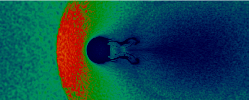
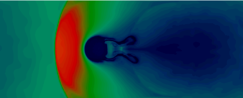
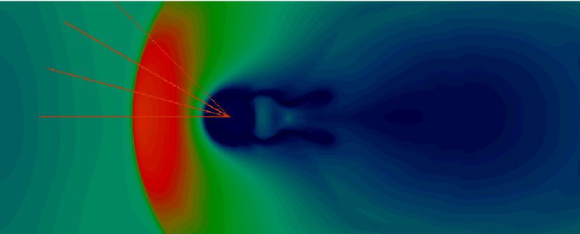
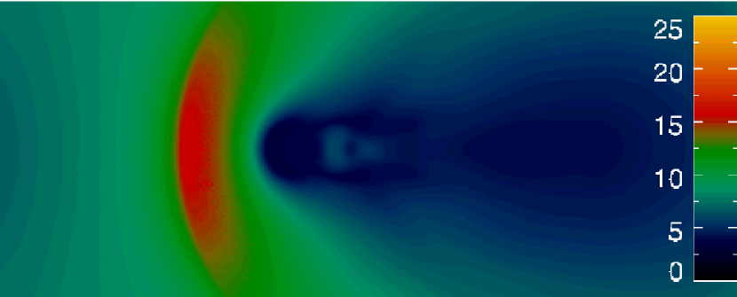
Figure 2: Snapshots of the temperature distribution for a 2D flow of hot (8 keV) gas past a cold (4 keV) cloud. The image sizes are 6.7 by 2.7 Mpc. The top panel corresponds to a moment shortly after the start of the simulations. In the other panels, the temperature distributions at $t=1.3\,{\rm Gyr}$ after the beginning of the simulations are shown as a function of the strength of thermal conduction. The conduction suppression coefficient for these panels is $f=0$, $0.01$, $0.1$, and $0.5$, respectively. Thus the second panel shows the run without conduction, while the bottom panel corresponds to a conductivity equal to half the Spitzer-Braginskii value. The temperature structure of the interface plotted in subsequent figures was measured along the red lines shown in one of the panels.

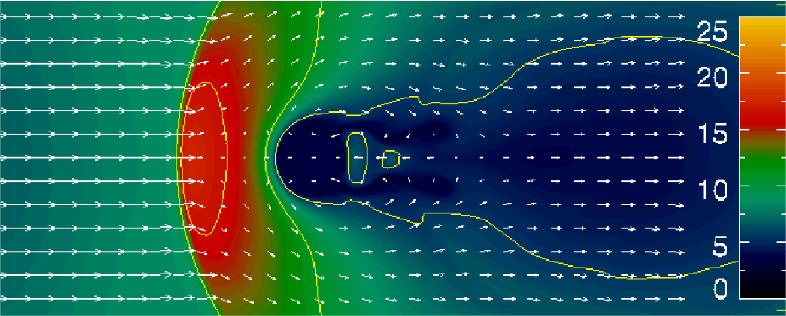
Figure 3: Snapshot of the temperature distribution at $t=1.3\,{\rm Gyr}$ after the start of a simulation with conductivity coefficient $f=0.1$, with the velocity field superposed.

Since after 1.3 Gyrs much of the relaxation from the initial state already took place, we compare the runs with different conductivity at this time. The effect of increasing the efficiency of thermal conduction is clearly visible in the snapshots shown in Fig. 2. First of all, small scale temperature variations present in the initial conditions are smoothed out in all runs where thermal conduction is present. Secondly, with the increase of $f$ the interface separating the cloud and the hot flow becomes less and less sharp. This is seen more explicitly in the temperature profiles across the interface (along the symmetry axis of the cloud), which are shown in Fig. 4. In this figure (and in the subsequent figures), the distance (plotted along the abscissa axis) is measured from the approximate centre of the cloud. Since the cloud is not perfectly spherical, its position varies slowly with time. As its centre is hence not accurately known, all profiles shown in Fig. 4 were shifted along the abscissa axis to have the temperature value 6 keV gas at the same position.

The sharpest profile corresponds of course to the run without conduction, and in this case some small-scale fluctuations left over from the initial conditions can still be seen in the profile. This run also sets a useful benchmark for comparison with the other simulations, for example, it indicates the numerical resolution available for representing the interface. We see that for values of $f$ larger than 0.01 the impact of thermal conduction on the width of the interface can be well resolved with our numerical setup. For runs with $f=0.01$, $0.1$ and $0.5$, the small-scale fluctuations in the temperature distribution are absent and the effective thickness of the interface gradually increases.

We can now verify our simple predictions based on the toy model of diffusion of a passive scalar in a potential flow. We first consider our finding that after an initial settling time of order $R/U$ the interface evolves to a quasi-steady state. This is indeed seen in Fig. 6, where the temperature profiles along the symmetry axis are shown for $t=0.2$, $0.4$, $0.8$, and $1.3\,{\rm Gyr}$ since the beginning of the simulations. While there is clear evolution of the profile (e.g. in terms of the maximal or minimal temperatures) the shape of the interface is very similar at all times.

Another expectation is that the thickness of the interface is the same along the interface (as long as the distance from the stagnation point is much less the the cloud curvature radius). Indeed, the profiles measured at different distances from the stagnation point (Fig. 7) look very similar. In this figure, the profiles were calculated along directions making different angle with respect to the symmetry axis of the cloud (red lines in Fig. 2). This means that when deriving an effective conduction coefficient from the observed cold fronts one can use the profile averaged over a large part of the interface, rather than being constrained to small sectors of the front.

Figure 4: Temperature profiles along the symmetry axis of the cloud at $t=1.3\,{\rm Gyr}$ after the start of the simulations, for different conduction suppression coefficients equal to $f=0$, $0.01$, $0.1$, and $0.5$. The distance is measured from the centre of the cold cloud.

Figure 5: Gas density profiles along the symmetry axis of the cloud at $t=1.3\,{\rm Gyr}$ after the start of the simulations, for different conduction suppression coefficients equal to $f=0$, $0.01$, $0.1$, and $0.5$. The distance is measured from the centre of the cold cloud.

Thus the results of the numerical simulations are broadly consistent with the expectations derived earlier: once the front is formed, it has a width constant in time and constant along the interface.

4 Simple estimates of the interface width

We are now looking for a simple 1D problem for a compressible fluid which has a solution that can provide a qualitative approximation of the cold front structure. The analogy with the problems considered in Section 2.2 suggests that the width of the interface should scale as $\sqrt{Dt_{s}}$, where $D$ is the effective diffusion coefficient (thermal conductivity) and $t_{s}$ is the effective time scale. For the flows in Section 2.2, a reasonable choice was $t_{s}\sim R/U$, where $R$ is the curvature radius of the interface and $U$ is the velocity of the flow at infinity. Of course, this result was derived for a potential flow, and for more realistic cases it might be more correct to recast $t_{s}$ in the form $t_{s}=\left(\frac{{\rm d}v_{r}}{{\rm d}r}\right)^{-1}$, where $v_{r}$ is the velocity component perpendicular to the interface. Indeed, from Eqs. (13) and (17) it is clear that that this quantity (i.e. the gradient of the radial velocity component) enters the expression of the interface width. We can hence try to obtain an approximate solution for the front structure by considering a 1D time dependent diffusion equation, starting from a Heaviside step function for the initial temperature distribution and taking the solution at time $t_{s}$. The hope is that for this choice of $t_{s}$ the most basic properties of the interface structure will be captured.

Figure 6: Temperature profiles along the symmetry axis of the cloud after $t=0.2$, $0.4$, $0.8$ and $1.3\,{\rm Gyr}$ since the start of the simulations. The conduction suppression coefficient was set to $f=0.1$. The distance is measured from the centre of the cloud. In order to compensate for the gradual changes in the interface shape, each profile was shifted along the X-axis so that the rising part of the temperature profile has the same abscissa for all curves.

We also assume that all velocities in the vicinity of the interface are small compared to the sound speed, all quadratic terms in $v$ can be neglected and that the pressure is approximately constant across the interface. Then the gas density is $\rho=\rho_{0}\frac{T_{0}}{T}$, where $\rho_{0}T_{0}=P_{0}$ is fixed by the initial pressure. In this approximation, the heat diffusion equation reduces to

$$\frac{\partial T}{\partial t}=\lambda\frac{\partial}{\partial x}k\frac{\partial T}{\partial x}-\lambda\frac{k}{T}\left(\frac{\partial T}{\partial x}\right)^{2},$$ (24)

where $\lambda=\frac{\gamma-1}{\gamma}\frac{\mu m_{p}}{\rho k_{B}}$. This equation is very similar to the standard diffusion equation in solids, except for the second term in the r.h.s. which accounts for gradual expansion of the heated gas, and for the contraction of the cooled gas in order to maintain constant pressure across the interface.

Figure 7: Temperature profiles at 1.3 Gyr for $f=0.1$ along directions making an angle of 0, 15, 30, or 45 degrees with respect to the symmetry axis of the cloud (see also Fig. 2).

Equation (24) can be readily integrated. We set the initial values of the temperature to 3 and 15 keV on the two sides of the interface, respectively, and the electron density to $10^{-2}\,{\rm cm}^{-3}$ on the cool side to approximately reproduce the properties of the simulated front, as shown in Fig. 7.

In Figure 8, we plot the solution of the equation at times $t=0.1$, $0.4$, $0.9$, and $2.0\,{\rm Gyr}$ for $f=0.1$ together with the temperature profile obtained in the SPH simulations. The results of the numerical simulations best correspond to the solution of Eqn. (24) for $t\sim 0.5-0.7\,{\rm Gyr}$. For comparison, the ratio of the cloud radius to the flow velocity at infinity is $R/U\sim 1.5\times 10^{8}$ yr, while $t_{s}$ evaluated from the velocity profile obtained in the simulations is $t_{s}=\left(\frac{{\rm d}v_{r}}{{\rm d}r}\right)^{-1}\approx 5\times 10^{8}\,{\rm yr}$. The difference in the estimated width of the front based on the $R/U$ ratio compared with a more detailed treatment of the velocity field is of order $2$. This discrepancy (for our numerical setup) is largely caused by i) the drop of the velocity at the shock and ii) differences between the velocity field obtained in the simulations and that in potential flows of incompressible fluids, as considered in Section 2.2. Of course, Eqn.(24) by itself is only a crude approximation of the problem. Nevertheless, even our simplest estimate predicts the width of the interface within a factor of 2 of the value derived from direct numerical simulations.

Note also that because of the expansion of the heated gas, the actual contact discontinuity does not necessarily exactly coincide with the “visible” boundary of the cool cloud. Indeed, colder gas of the cloud expands while the hotter ambient gas contracts, shifting the discontinuity away from the cloud centre. At the same time, the sharpest edge will be observed in places where the temperature gradient is large. If the gas on the two sides of the contact discontinuity has different abundances of heavy elements then the true position of the contact discontinuity can be determined from the abundance gradient. This exercise however requires data of very high quality.

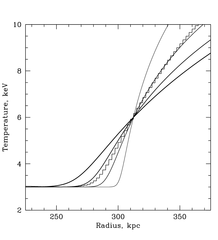
Figure 8: Comparison of the temperature profile along the symmetry axis of the cloud (for $f=0.1$) obtained in numerical simulations (histogram) and obtained from equation (24) for $t_{s}=0.1$, $0.4$, $0.9$, and $2.0\,{\rm Gyr}$.

We thus find that an order of magnitude estimate of the width of a spherical cold front can be written as

$$\Delta r\approx\delta\sqrt{\frac{2}{3}D\frac{R}{U}}=\delta\sqrt{\frac{2}{3}\frac{\gamma-1}{\gamma}\frac{\mu m_{p}}{\rho}\frac{fk_{0}}{k_{B}}\frac{R}{U}},$$ (25)

where the factor $\delta$ accounts for all departures introduced by the approximations involved in our simplest model considered in Section 2.2. Based on our numerical simulations we have $\delta\sim 0.5$. Plugging in fiducial values for the A3667 cluster (Vikhlinin et al., 2001) one gets:

$$\Delta r\approx 40\left(\frac{\delta}{0.5}\right)f^{0.5}T_{5}^{5/4}R_{300}^{0.5}U_{1400}^{-0.5}N_{0.002}^{-0.5}~{}\;{\rm kpc},$$ (26)

where $T_{5}=\frac{T}{5\,{\rm keV}}$, $R_{300}=\frac{R}{300\,{\rm kpc}}$, $U_{1400}=\frac{U}{1400\,{\rm km\,s^{-1}}}$, and $N_{0.002}=\frac{n_{e}}{2\times 10^{-3}\,{\rm cm}^{-3}}$.

This value is a factor of $\sim 8$ larger than the upper limit for the interface width derived from Chandra observations. If this discrepancy is solely caused by a suppression of thermal conduction, then the factor $f$ has to be less than $1.5\times 10^{-2}$. Note that the mean free path is $\lambda\sim 4~{}T_{5}^{2}N_{0.002}^{-1}\,{\rm kpc}$ (e.g. Sarazin, 1986), which is smaller than the interface width evaluated for $f=1$. If the effective mean free path of electrons scales linearly with $f=k/k_{0}$ (while the interface width $\Delta r\propto\sqrt{f}$) then for all $f<1$ the width of the interface will remain larger than the mean free path. Therefore our assumption of unsaturated heat flux remains valid. For the observed cold front in A3667 the effective mean free path of electrons should therefore be factor $f=1.5\times 10^{-2}$ smaller than in unmagnetized plasma.

However, we caution that magnetic fields are likely playing a role in the structure of the interface as suggested by theoretical arguments (e.g. Vikhlinin et al., 2001, Lyutikov 2006) and numerical simulations (e.g. Asai 2004, 2005). Particularly important is the stretching of the field lines along the interface, which can suppress heat conduction across the front or even affect the hydrodynamical stability of the interface. Note that the heat conductivity depends strongly on the topology of the magnetic field since the electron Larmor radius is some 10 orders of magnitude smaller than the characteristic length scales of the problem for typical magnetic field strengths at the micro-Gauss level.

We note that the interface developing in our SPH simulations may also be stabilized to some extent against small-scale fluid instabilities by numerical effects. Across strong density discontinuities, SPH has been found to produce spurious pressure forces that may suppress small wavelength Kelvin-Helmholtz instabilities (Agertz et al. 2006). This effect is equivalent to a small surface tension and mimics the stabilizing influence expected from an ordered magnetic field across the front. However, better numerical resolution weakens this effect and should allow ever smaller wavelengths to grow.

5 Conclusions

We have shown that in the presence of thermal conduction the width of the interface separating hot gas flowing past a cooler gas cloud (a “cold front” in clusters of galaxies) can be estimated from the size $R$ of the cloud, the velocity $U$ of the gas and the effective thermal conductivity. The structure of the interface is established over a period of time $\sim R/U$, while the subsequent evolution is much slower. Moreover, the width of the interface is approximately constant along the front. We made an illustrative 2D simulations of an unmagnetized plasma flow past a colder cloud with gas densities and temperatures characteristic for the observed cold fronts. While being very idealized, the simualtions do show that the width remains approximately constant when the gas compressiblity and the temperature dependence of the conductivity is accounted for.

This implies that one can use much of the visible part of the interface in order to assess the effective thermal conductivity of the gas. For the cold front in Abell 3667, the estimated width of the interface is $40f^{0.5}~{}{\rm kpc}$, where $f$ is the conduction suppression coefficient (relative to the Spitzer-Braginskii value). This factor $f$ has to be smaller than $0.015$ in order to reproduce the observed limits on the width of the interface. This result is consistent with previous suggestions that magnetic fields play an important role in providing thermal isolation of the gases separated by the cold front. The idealised description of the interface presented here provides a useful method for estimating the effective gas conductivity from observations of clusters of galaxies.

References

- [Acreman et al.(2003)] Acreman, D. M., Stevens, I. R., Ponman, T. J., & Sakelliou, I. 2003, MNRAS, 341, 1333
- [Agertz et al.(2006)] Agertz et al. 2006, astro-ph/0610051
- [Asai et al.(2004)] Asai N., Fukuda N., & Matsumoto R. 2004, ApJL, 606, L105
- [Asai et al.(2005)] Asai N., Fukuda N., & Matsumoto R. 2005, Advances in Space Research, 36, 636
- [Asai et al.(2007)] Asai, N., Fukuda, N., & Matsumoto, R. 2007, ArXiv Astrophysics e-prints, arXiv:astro-ph/0703536
- [Batchelor 1967] Batchelor G.K., An Introduction to Fluid Dynamics, CUP, Cambridge, 1967
- [Bialek et al.(2002)] Bialek, J. J., Evrard, A. E., & Mohr, J. J. 2002, ApJL, 578, L9
- [braginskii et al.(2005)] Braginskii S.I., in Reviews of Plasma Physics, edited by Leontovich M.A. (Consultants Bureau, New York, 1965)