Quantum geometry and gravitational entropy

Most quantum states have wavefunctions that are widely spread over the accessible Hilbert space and hence do not have a good description in terms of a single classical geometry. In order to understand when geometric descriptions are possible, we exploit the AdS/CFT correspondence in the half-BPS sector of asymptotically ${\rm AdS}_{5}\times S^{5}$ universes. In this sector we devise a “coarse-grained metric operator” whose eigenstates are well described by a single spacetime topology and geometry. We show that such half-BPS universes have a non-vanishing entropy if and only if the metric is singular, and that the entropy arises from coarse-graining the geometry. Finally, we use our entropy formula to find the most entropic spacetimes with fixed asymptotic moments beyond the global charges.

1 Introduction

The $\frac{1}{2}$-BPS sector of $\mathcal{N}=4$ $\textrm{SU}(N)$ Yang–Mills theory provides a simple playground for understanding quantum gravity, as the semiclassical mapping between spacetime geometries and coherent field theoretic states is particularly simple [2, 4, 6, 8, 10, 12, 14]. Here we propose an extension of this mapping to the quantum level. Using a second-quantized formalism, we define a ‘metric’ operator in the Yang-Mills theory whose eigenstates map to universes with a single well-defined topology and geometry, while non-eigenstates do not have a good description in terms of single spacetimes.

In the field theory, the half-BPS states can be constructed by reducing the $\textrm{SU}(N)$ Yang-Mills Lagrangian to a Hermitian matrix model and studying its Hilbert space [6, 8]. This in turn has a description in terms of $N$ fermions in a harmonic potential. Approximate eigenstates of our metric operator can be constructed by placing the individual fermions in coherent states. (See [12, 14] for a related discussion in the ${\rm AdS}_{3}$ context.) Using this formalism, we can associate an entropy to any classical, asymptotically ${\rm AdS}_{5}\times\textrm{S}^{5}$ spacetime in the LLM family given by [2], by counting how many microscopic configurations give the same coarse-grained metric. We find that only the singular spacetimes have a finite entropy; thus spacetime singularities and the appearance of gravitational entropy are intimately tied together, at least within the class of LLM geometries. By studying the partition sum over geometries we show that only the smooth spacetimes appear in the underlying configuration space, which is thus effectively discretized. This provides further evidence that singularities and their associated entropy arise only in passing to our long-distance effective description. Our formalism can be used to determine the most entropic geometries with specified angular moments; in essence, this extends the extremal “superstar” black hole geometry to black objects carrying higher angular moments.

The data required for constructing the metric in these half-BPS universes can be extracted from the effective single-particle phase space distribution of the fermionic representation of the half-BPS matrix model. This procedure generically loses information about the complete state, which is fully represented in an $N$-particle phase space. Hence the semiclassical geometry will generally lose information about the underlying quantum state. We show that in the semiclassical limit ($N\to\infty$) this sort of information loss occurs if and only if the metric is singular.

While this paper was in preparation we received [16] which has substantial overlap with some sections of this paper, and [18] which carries out similar analyses of the entropy of coarse-grained BPS spacetimes in other settings.

2 Half-BPS states: review and set up

Gravity:

Type IIB string theory in 10 dimensions has a family of asymptotically ${\rm AdS}_{5}\times S^{5}$ solutions that preserve 16 supercharges; these are the $\frac{1}{2}$-BPS states. Of particular interest are the subset of states that preserve an additional $\textrm{SO}(4)\times\textrm{SO}(4)$ symmetry. All states in this subset were written down in [2] and are of the form

$$ds^{2}=-h^{-2}\,(dt+V_{i}dx^{i})^{2}+h^{2}\,(dy^{2}+dx^{i}dx^{i})+R^{2}\,d\Omega_{3}^{2}+\tilde{R}^{2}\,d\tilde{\Omega}_{3}^{2},$$ (1)

where the coefficients are given by

$$R^{2}=y\,\sqrt{\frac{1-u}{u}},\quad\tilde{R}^{2}=y\,\sqrt{\frac{u}{1-u}},\quad h^{-2}=\frac{y}{\sqrt{u(1-u)}},$$ (2)

and are entirely specified by the function $u(x_{1},x_{2},y)$. The one-form field $V$ can also be given in terms of $u$, but it will not be needed here. Note that $x_{1}$ and $x_{2}$ have units of length squared. This function in turn solves a harmonic equation in $y$ and is determined by its boundary condition on the $y=0$ plane

$$u(x_{1},x_{2})\equiv u(x_{1},x_{2},0)\,.$$ (3)

(We will frequently drop the arguments and simply call this function $u$.) On this space of solutions it can be shown [2] that the Hamiltonian is

$$H=\int{d^{2}x\over 2\pi\hbar}{x_{1}^{2}+x_{2}^{2}\over 2\hbar}\,u(x_{1},x_{2})\,.$$ (4)

The flux of $F_{5}$ passing through the asymptotic $S^{5}$ in such spaces is

$$N=\int{d^{2}x\over 2\pi\hbar}\,u(x_{1},x_{2})$$ (5)

It turns out that the solutions (1) are singular unless $u(x_{1},x_{2})=0,1$ everywhere. When $u>1$ or $u<0$ the solutions have closed timelike curves [19], so we will always take $0\leq u\leq 1$.

Field theory:

In the dual ${\cal N}=4$ $\textrm{SU}(N)$ Yang-Mills theory on $S^{3}\times R$ the corresponding states preserve 16 supersymmetries. Due to the BPS condition these states are constant on the $\textrm{S}^{3}$, leading to an $\textrm{SO}(4)$ symmetry. When one constructs states using only one of the three complex scalar fields, the internal $\textrm{SO}(6)$ R-symmetry is broken to $\textrm{SO}(4)$. Thus these states have the same symmetries as the gravity solutions described above.

It has been shown [6, 8] that all of these states can be described in terms of a matrix model for the one homogenous mode of the complex adjoint scalar field:

$$S_{{\rm YM}}={1\over g^{2}_{YM}}\int dt\left({1\over 2}\dot{X}^{2}+{1\over 2}X^{2}\right)\,.$$ (6)

The dictionary relating that Yang-Mills theory to string theory ensures that

$$\hbar\leftrightarrow\ell_{P}^{4}$$ (7)

where $\hbar$ is Planck’s constant governing the semiclassical limit of (6) and $\ell_{P}$ is the 10 dimensional Planck length governing the semiclassical limit on the gravity side. The matrix model (6) can be solved in the usual way by going to the eigenvalue basis, in which case it reduces to a system of $N$ non-interacting fermions in a harmonic potential. A basis for the Hilbert space is specified by a set of non-decreasing integers

$$r_{i}=\frac{E_{i}}{\hbar}-i+1/2,~{}~{}~{}i=1,2,\cdots N$$ (8)

which measure the excitation of each fermion above the vacuum. The data $\{r_{i}\}$ may be summarized in a Young diagram in which the ${\rm i}^{\rm th}$ row has length $r_{i}$. In the semiclassical limit, it has been proposed that these states are mapped to the dual solutions (1) with the identification [10]

$$u(x_{1},x_{2})\leftrightarrow\hbar\,W(p,q)~{};~{}~{}~{}~{}~{}~{}~{}(x_{1},x_{2})\leftrightarrow(p,q)$$ (9)

where $W(p,q)$ is the semiclassical density of fermions in the single particle harmonic oscillator phase plane $(p,q)$. There are many different quantum mechanical density functions on phase space; however, all well-defined phase space distributions share the same semiclassical limit. Thus we will mostly work with the well-known Wigner density function (see Appendix A) and occasionally with the Husimi distribution (see Sec. 3.2.1) that is obtained by convolving the Wigner distribution with a coherent state [10].

Integrable charges:

In [21] we pointed out that the half-BPS sector of ${\cal N}=4$ Yang-Mills theory is integrable and thus has a family of higher Hamiltonians

$$M_{k}={\rm Tr}(H_{N}^{k}/\hbar^{k})=\sum_{i=1}^{N}\lambda_{i}^{k}~{}~{}~{}~{};~{}~{}~{}~{}k=0,\cdots N$$ (10)

where $H_{N}$ is the Hamiltonian in the free fermion Hilbert space and $\lambda_{i}=\frac{E_{i}}{\hbar}$ is the energy of the $i^{th}$ fermion in units of $\hbar$. This can be written in terms of a phase space integral, and using the correspondence with spacetime (9), becomes

$$M_{k}=\int\frac{d^{2}x}{2\pi\hbar}\frac{(x_{1}^{2}+x_{2}^{2})^{k}}{2^{k}\hbar^{k}}u(x_{1},x_{2}),$$ (11)

which is accurate to leading order in $N$.

Any eigenstate of this tower of conserved charges can be completely identified by measurement of all the eigenvalues. In [21] we showed that in the semiclassical limit these higher Hamiltonians can be read off from the asymptotic angular moments of the spacetime. Specifically, the k^th angular moment of the function $u(x_{1},x_{2},y)$ that appears in (1) is proportional to the expected value of $M_{k}$:

$$u(\rho,\theta,\varphi)=2\cos^{2}\theta\sum_{k=0}^{\infty}\frac{2^{k}\langle M_{k}\rangle}{\rho^{2k+2}}\,(-1)^{k}(k+1)\,\,{{}_{2}F_{1}}(-k,k+2,1;\sin^{2}\theta).$$ (12)

where $\rho^{2}=y^{2}+r^{2}$, $y$ is the transverse direction to the $(x_{1},x_{2})$ plane, $r$ is the radial direction in this plane and $\theta$ is the angle between the plane and the transverse direction measured by $\rho$. Nevertheless, it turns out that in typical states with a given total energy ($M_{1}$), Planck scale measurements are required to distinguish between the microstates. Hence information about these states is lost in the semiclassical limit.

3 Quantum geometry

The naive correspondence (9) associates a geometry to every state in the Hilbert space via the phase space fermion density in the free fermi description of the half-BPS states. The correspondence cannot be correct in this naive form – while a suitably coherent state in the field theory can correspond to a semiclassical geometry, there will be many states which correspond to wavefunctions that have support on spacetimes of widely different geometry and topology. Thus it is of interest to identify which field theory states have a description in terms of a single classical geometry vs. a superposition of geometries. In this section, we will define a ‘metric’ operator in the Yang-Mills theory and propose that the eigenstates of this operator are the ones that can be mapped to semiclassical geometries using (9), while the non-eigenstates cannot be associated to a unique metric in this manner.

3.1 Four ways of becoming a superstar?

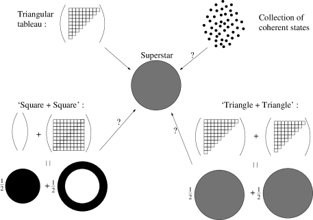
Figure 1: Four CFT states naively would be mapped to the superstar.

To illustrate the difficulty with the naive correspondence (9) we will consider different ways in which the extremal half-BPS black hole (the “superstar” [22]) would be generated by applying (9) to field theory states. It was shown in [2, 10] that the metric (1) realizes the superstar geometry when the function $u(x_{1},x_{2})$ (3) takes a constant value between 0 and 1 within a circular droplet in the $(x_{1},x_{2})$ plane, and vanishes outside it. This $u$ function is depicted in the center of Fig. 1. It was also shown that a fermion basis state (8) described by a triangular Young tableau (upper left corner of Fig. 1) has a phase space density of this form, and hence corresponds to a superstar geometry according to (9).

We will now examine other states in the field theory that have the same single particle Wigner distribution. For definiteness, we choose, without loss of generality, to work with a droplet with $u(x_{1},x_{2})=\frac{1}{2}$ inside the droplet. In terms of the triangular tableau, this corresponds to having an equal number of rows and columns ($N=N_{c}$) [10], while for the superstar this means that the number of giant gravitons sourcing the geometry is equal to the flux of the five-form field [22]. The radius of the droplet for this configuration is $\sqrt{2}R_{AdS}^{2}$. In terms of excitation numbers the triangular tableau state is given by

$$|\textrm{`triangle'}\rangle=|0,2,4,\ldots,2(N-1)\rangle.$$ (13)

Another way of producing the superstar is to place the $N$ fermions in the field theory in coherent states that are randomly distributed in phase space inside the circle of radius $\sqrt{2}R_{AdS}^{2}$ (upper right corner, Fig. 1). Since coherent states are minimum uncertainty packets, as we will see in Secs. 3.3 and 4, they will cover half the area contained inside the circle. Upon coarse graining at the $\hbar$ scale, this configuration has a phase space distribution that is $\hbar W=1/2$ inside the circle and $\hbar W=0$ outside. Upon using the correspondence (9) we once again recover the superstar geometry.

Thirdly, we can consider a superposition of two very similar triangles, one with even excitations and one with odd excitations (Fig. 1; bottom right):

$$|\textrm{{`triangle + triangle'}}\rangle = \frac{1}{\sqrt{2}}|0,2,\ldots,2N-2\rangle+\frac{1}{\sqrt{2}}|1,3,\ldots,2N-1\rangle$$ (14)

$$\equiv \frac{1}{\sqrt{2}}|\textrm{`evens'}\rangle+\frac{1}{\sqrt{2}}|\textrm{`odds`}\rangle.$$

And finally, we can consider the superposition of the empty tableau corresponding to the $AdS$ vacuum, and a square tableau of size $N_{c}\times N$ (Fig. 1; bottom left):

$$|\textrm{{`square + square'}}\rangle = \frac{1}{\sqrt{2}}|0,1,\ldots,N-1\rangle+\frac{1}{\sqrt{2}}|N,N+1,\ldots,2N-1\rangle$$ (15)

$$\equiv \frac{1}{\sqrt{2}}|0\rangle+\frac{1}{\sqrt{2}}|N\times N_{c}\rangle.$$

The last two superpositions are also depicted in figure 1. Computing the corresponding phase space distributions (following [10] or (64) later in this paper) one can see that the phase space distributions corresponding to these states will indeed reproduce the superstar geometry upon coarse graining.

The last two cases are both simple superpositions of basis states. However, the ‘square + square’ example is more dramatic as it is a superposition of states of vastly different energies, unlike ‘triangle + triangle’. The energy associated to the $AdS$ vacuum is $\frac{N^{2}}{2}$, while the energy of the $N\times N_{C}$ tableau is $\frac{3N^{2}}{2}$ for $N=N_{c}$, yielding an average energy of $N^{2}$. As soon as an observer performs even a rough measurement of the energy, the universe is projected into one of the two energy eigenstates. On the gravity side, the corresponding geometries differ from each other (and from the superstar!) at scales that are easily measurable, since the relevant scale is roughly the $AdS$ radius $R_{AdS}$. Thus, ‘square + square’ does not describe anything like a classical superstar, and can only be described as a superposition of distinct geometries. We wish to develop a formalism that can distinguish states of this sort from the ones that can be usefully mapped to a unique metric.

3.2 The second quantized formalism

It will be convenient to use a second quantized description of the fermion system. For each state $\psi$ in the 1-particle Hilbert space ${\cal H}_{1}$, we define both a fermion creation operator $b^{\dagger}(\psi)$ and a fermion annihilation operator $b(\psi)$ which satisfy

$$\{b(\psi_{1}),b(\psi_{2})\}=0,$$ (16)

$$\{b^{\dagger}(\psi_{1}),b^{\dagger}(\psi_{2})\}=0,$$ (17)

$$\{b(\psi_{1}),b^{\dagger}(\psi_{2})\}=\langle\psi_{1}|\psi_{2}\rangle,$$ (18)

where the inner product on the right is taken in ${\cal H}_{1}$. Since we deal with free fermions, the anti-commutators on the left-hand side of equations (18) are proportional to the identity. Thus it makes sense to set them equal to the complex numbers on the right-hand side.

We will in particular be interested in the case where $\psi$ is a coherent state labelled by a parameter $\alpha\in{\mathbb{C}}$. In phase space these states manifest themselves as gaussian wavepackets localized around $\alpha=\frac{x_{1}+i\,x_{2}}{\sqrt{2\hbar}}$, and are defined by

$$|\alpha\rangle=e^{-|\alpha|^{2}/2}\sum_{n=0}^{\infty}\frac{\alpha^{n}}{\sqrt{n!}}|n\rangle\equiv\sum_{n=0}^{\infty}c_{n}(\alpha)|n\rangle\,.$$ (19)

These form an overcomplete basis, and have overlaps

$$\langle\beta|\alpha\rangle=\exp\left(-\frac{|\alpha|^{2}+|\beta|^{2}-2\beta^{*}\alpha}{2}\right)\,.$$ (20)

Throughout this section, the normalization conventions are as in [20]. We shall abuse notation somewhat by taking $b^{\dagger}(\alpha),b(\alpha)$ to represent the creation and annihilation operators corresponding to the coherent state determined by $\alpha\in{\mathbb{C}}$. The simple form and well-known properties of the coherent state (19) provide a convenient foundation upon which to base a semiclassical formalism. We make use of this opportunity in the rest of this work. However, in section 7, we describe certain desirable improvements which, unfortunately, will come with increased technical complications.

We wish to define a ‘metric’ operator in the field theory with the property that its eigenstates are well described by a single classical metric which is in turn given by the eigenvalue of the operator. Since any 1/2-BPS metric may be expressed in terms of the function $u(x_{1},x_{2})$, it is enough to define an operator $\hat{u}(x_{1},x_{2})$ in terms of the fermion operators; we can take all other metric operators to be given by the classical LLM formulae with $u$ replaced by $\hat{u}$. We will see that, with our definition of $\hat{u}$ below, such expressions will require no regularization.

For $\alpha=\frac{x_{1}+ix_{2}}{\sqrt{2\hbar}}$, we make the definition

$$\hat{u}(\alpha)\equiv b^{\dagger}(\alpha)b(\alpha),$$ (21)

and $\hat{u}(x_{1},x_{2})\equiv\hat{u}(\frac{x_{1}+ix_{2}}{\sqrt{2\hbar}})$. Thus, for each $\alpha$ the operator $\hat{u}(\alpha)$ is a fermion number operator, having eigenvalues 0 and 1.

Our definition satisfies a number of useful properties. For example, we have

$$\hat{N} = \int\frac{dx_{1}dx_{2}}{2\pi\hbar}\,\hat{u}(x_{1},x_{2}),\ \ \ {\rm and}$$ (22)

$$\hat{H} = \int\frac{dx_{1}dx_{2}}{2\pi\hbar}\frac{x_{1}^{2}+x_{2}^{2}}{2\hbar}\,\hat{u}(x_{1},x_{2}),\ \ \ {\rm and}$$ (23)

$$\hat{M}_{k} = \int\frac{dx_{1}dx_{2}}{2\pi\hbar}\left(\frac{x_{1}^{2}+x_{2}^{2}}{2\hbar}\right)^{k}\hat{u}(x_{1},x_{2}).$$ (24)

These are precisely the relations which hold between the corresponding classical quantities.

Furthermore, one may show that these $\hat{u}(\alpha)$ generate a complete set of operators which do not change fermion number. Here the essential point is that any operator on the 1-particle Hilbert space can be expressed in the form $\int d^{2}\alpha f(\alpha)|\alpha\rangle\langle\alpha|$. Now, if $|\psi_{n}\rangle$ denotes the ${\rm n}^{\rm th}$ energy level of the 1-particle harmonic oscillator, we may define a complex function $f_{nm}(\alpha)$ by

$$|\psi_{n}\rangle\langle\psi_{m}|=\int\!\!\!\int d^{2}\alpha f_{nm}(\alpha)|\alpha\rangle\langle\alpha|.$$ (25)

It is then straightforward to show that

$$b^{\dagger}(\psi_{n})b(\psi_{m})=\int\!\!\!\int d^{2}\alpha f_{nm}(\alpha)\hat{u}(\alpha).$$ (26)

It is clear that any operator which preserves particle number can be built by taking sums of products of $b^{\dagger}(\psi_{n})b(\psi_{m})$, and thus that any such operator can be built from $\hat{u}(\alpha)$.

3.2.1 $\hat{u}$ and the Husimi distribution

We now wish to connect the operator $\hat{u}$ to a semi-classical phase space distribution function by showing that the expectation value of $\hat{u}$ in a general state $|\Psi\rangle$ is the Husimi distribution on phase space:

$$\langle\Psi|\hat{u}(\alpha)|\Psi\rangle=\pi\textrm{Hu}^{\rho_{1}}(\alpha),$$ (27)

where $\textrm{Hu}^{\rho_{1}}(\alpha)$ is the Husimi distribution corresponding to the one particle density matrix $\hat{\rho}_{1}$ associated to $|\Psi\rangle$. To show this, we write the general state as a superposition of basis states as

$$|\Psi\rangle=\sum_{w}d_{w}|\mathcal{F}^{w}\rangle,$$ (28)

where $w$ sums over the basis states in the superposition, the normalization is $\sum_{w}|d_{w}|^{2}=1$ and $\mathcal{F}^{w}$ is the set of excitation numbers characterising a basis state $|\lambda_{1}^{w},\ldots,\lambda_{N}^{w}\rangle$. The basis states in turn are given by

$$|\lambda_{1},\ldots,\lambda_{N}\rangle=b^{{\dagger}}(\lambda_{1})\ldots b^{{\dagger}}(\lambda_{N})|0\rangle.$$ (29)

Using the commutators (18) one can show that

$$\langle\Psi|\hat{u}(\alpha)|\Psi\rangle=\sum_{w,w^{\prime}}d^{*}_{w^{\prime}}d_{w}\sum_{i_{w},j_{w^{\prime}}=1}^{N}(-1)^{i_{w}+j_{w^{\prime}}}\langle\lambda_{j^{w^{\prime}}}^{w^{\prime}}|\alpha\rangle\langle\alpha|\lambda_{i^{w}}^{w}\rangle\langle 0|\prod_{\stackrel{{\scriptstyle k=1}}{{k\neq i_{w}}}}^{N}b(\lambda_{k}^{w^{\prime}})\prod_{\stackrel{{\scriptstyle l=1}}{{l\neq j_{w}}}}^{N}b^{{\dagger}}(\lambda_{l}^{w})|0\rangle$$

$$=\sum_{w}|d_{w}|^{2}\sum_{i_{w}=1}^{N}|\langle\alpha|\lambda_{i^{w}}^{w}\rangle|^{2}+\sum_{(w,w^{\prime})\in\mathcal{C}}d_{w}d_{w^{\prime}}^{*}(-1)^{N^{(w,w^{\prime})}+N^{(w^{\prime},w)}}\langle\lambda_{(w^{\prime},w)}|\alpha\rangle\langle\alpha|\lambda_{(w,w^{\prime})}\rangle.$$ (30)

The expectation value on the right side of the first line can clearly be nonzero only when at least $N-1$ of the excitation numbers in $\mathcal{F}^{w}$ and $\mathcal{F}^{w^{\prime}}$ are the same. This allowed us to simplify the expression at the cost of introducing some new notation. In the above, $\mathcal{C}$ denotes the set of pairs of states that differ from each other by one excitation, and for each such pair we define the excitation to be $\{\lambda_{(w,w^{\prime})}\}=\mathcal{F}^{w}\backslash\mathcal{F}^{w^{\prime}}$. Finally, $N^{(w,w^{\prime})}$ indexes the number of the differing excitation, i.e. if $\lambda_{(w,w^{\prime})}=f_{i}^{w}\in\mathcal{F}^{w}$, then $N^{(w,w^{\prime})}=i$.

Next we need to evaluate the right hand side of (27), and thus we recall the definition of the Husimi distribution from [20]:

$$\textrm{Hu}^{\rho_{1}}(\alpha)=\frac{1}{\pi}\langle\alpha|\hat{\rho}_{1}|\alpha\rangle.$$ (31)

The one particle density matrix corresponding to $|\Psi\rangle$ can be easily found by tracing over $N-1$ of the particles. Due to the orthogonality, the trace can also be nonzero only if at least $(N-1)$ of the excitations are the same, and after a little work we get

$$\hat{\rho}_{1}=N\,\textrm{Tr}_{\mathcal{H}_{2}\otimes\ldots\mathcal{H}_{N}}(|\Psi\rangle\langle\Psi|)=\sum_{w}|d_{w}|^{2}\sum_{i_{w}=1}^{N}|\lambda_{i^{w}}^{w}\rangle\langle\lambda_{i^{w}}^{w}|+$$

$$+\sum_{(w,w^{\prime})\in\mathcal{C}}d_{w}d_{w^{\prime}}^{*}(-1)^{N^{(w,w^{\prime})}+N^{(w^{\prime},w)}}|\lambda_{(w,w^{\prime})}\rangle\langle\lambda_{(w^{\prime},w)}|,$$ (32)

and plugging this into (31) we immediately recover (27).

3.3 A coarsegrained $\hat{u}$ and its eigenstates

The metric operator $\hat{u}$ is not well suited to a semiclassical observer, since it is very sensitive to details at the Planck scale. Thus, we wish to coarse grain it over some distance scale $L$. To do this, we’ll compute a convolution with a Gaussian kernel:

$$\tilde{u}(x_{1},x_{2})=\frac{1}{\pi L^{2}}\int\!\!\!\int dx^{\prime}_{1}\,dx^{\prime}_{2}\,e^{-\frac{(x_{1}-x^{\prime}_{1})^{2}+(x_{2}-x^{\prime}_{2})^{2}}{L^{2}}}\hat{u}(x^{\prime}_{1},x^{\prime}_{2}).$$ (33)

Since this operator is essentially a weighted average of local values of $\hat{u}$, it will have a continuous spectrum of eigenvalues between 0 and 1 and it is not sensitive to details at the Planck scale. This operator valued function on the single fermion phase space is our proposal for a “metric operator”, namely the operator whose eigenstates can be associated to semiclassical geometries using the LLM prescription.

To make this more precise, we next need to define exactly what me mean by eigenstates and the semiclassical limit. The semiclassical limit can be defined simply as

$$\ell_{P}\to 0~{}~{}~{}~{};~{}~{}~{}~{}L\to 0~{}~{}~{}~{};~{}~{}~{}~{}{L\over\ell_{P}}\to\infty.$$ (34)

We can see that the commutator $[\tilde{u}(\alpha),\tilde{u}(\beta)]$ does not vanish, though it approaches zero rapidly when $\alpha$ and $\beta$ are separated by more than a distance $L$. As a result, only states which are eigenstates of the $\hat{u}(\alpha)$ with eigenvalue $0$ or $1$ for all $\alpha$ (i.e. states with an empty or completely filled phase plane) can be exact eigenstates of $\tilde{u}$. Neither of these possibilities is of interest. Other states are only approximate eigenstates. For example, consider empty AdS space, the vacuum of the theory. In terms of Young tableaux for fermion excitation energies, AdS space is described as the empty tableau and the correspondence phase space density is the filled fermi sea, i.e. a filled disk of fermions in phase space. For $|\alpha|$ well within the filled disk, the state is an approximate eigenstate of $\tilde{u}(\alpha)$ with eigenvalue one. When $|\alpha|$ is well outside the black disk, the state is an approximate eigenstate of $\tilde{u}(\alpha)$ with eigenvalue zero. However, when $\alpha$ is within $L$ of the boundary, the state is far from being an eigenstate of $\tilde{u}(\alpha)$.

Thus we will define approximate eigenstates as follows: We say that a state $|\Psi\rangle$ is an approximate eigenstate of $\tilde{u}(\alpha)$ with eigenvalue function $u(\alpha)$ and a given accuracy $\epsilon$, if and only if

$$\int d^{2}\alpha\left|\big{(}\tilde{u}_{N}(\alpha)-u(\alpha)\big{)}|\Psi\rangle\right|^{2}<\epsilon.$$ (35)

With this definition we can easily see that of the four aspiring superstars introduced earlier, only ‘square + square’ is not an approximate eigenstate of $\tilde{u}$ thus shouldn’t be associated with the superstar geometry.

Armed with the definition of eigenstates of the coarse-grained $\tilde{u}$, such eigenstates can be associated with a slowly-varying density function which we have called $u(\alpha)$, and it is in terms of this function that we shall now discuss the thermodynamics and entropy of these solutions.

4 Entropy of BPS geometries

Following Sec. 3.2 all eigenstates of the metric operator can be constructed by placing each fermion in the free-fermi description of half-BPS states in a coherent state in phase space. It is known that coherent states placed on an $\hbar$-spaced lattice in phase space also provide a complete basis for the Wigner distributions in the single-particle phase space [23], and hence, by (9) for all semiclassical geometries. Because of the coarse-graining, many different quantum states may have the same geometrical description. Thus some geometries should be associated to an entropy, whose exponential counts the number of underlying states with the same geometric description. In this section we want to find a formula for the entropy of half-BPS spacetimes and then use it to discuss the partition sum over these geometries. With this motivation we will construct the Wigner distribution of the coherent state basis for half-BPS states and coarse-grain that to find our formula for the entropy of half-BPS semiclassical spacetimes.

4.1 Coherent states and entropy

The semiclassical limit of half-BPS states in Yang-Mills theory is most conveniently studied in terms of coherent states (19), rather than the energy eigenstates described above. Each of the $N$ fermions in the harmonic potential can be placed separately in a coherent state, with the fermionic statistics imposed by a Slater determinant.

Consider an $N$-particle (unnormalized) wavefunction given by antisymmetrizing 1-particle wavefunctions $\Psi_{i}(x_{j})$, $i,j=1\ldots N$:

$$\Psi(x_{1},\ldots,x_{N})=\det\left[\begin{array}[]{cccc}\Psi_{1}(x_{1})&\Psi_{1}(x_{2})&\cdots&\Psi_{1}(x_{N})\\ \Psi_{2}(x_{1})&\Psi_{2}(x_{2})&\cdots&\Psi_{2}(x_{N})\\ \vdots&&&\\ \Psi_{N}(x_{1})&\Psi_{N}(x_{2})&\cdots&\Psi_{N}(x_{N})\end{array}\right]=\sum_{\sigma\in S_{N}}(-)^{\sigma}\prod_{i}^{N}\Psi_{\sigma(i)}(x_{i}).$$ (36)

The 1-particle-reduced density matrix of this state is

$$\hat{\rho}_{1}=\frac{N\int dx_{2}\ldots dx_{N}|\Psi\rangle\langle\Psi|}{\langle\Psi|\Psi\rangle}=\sum_{mn}|\Psi_{m}\rangle\rho_{mn}\langle\Psi_{n}|\,.$$ (37)

In terms of the quantities

$$\hat{D}(\xi) = e^{\xi\hat{\alpha}^{\dagger}-\xi^{*}\hat{\alpha}}\,,$$ (38)

$$\chi(\xi) = {\rm tr}(\hat{\rho}_{1}\hat{D}(\xi))\,,$$ (39)

the Wigner phase space distribution of $|\Psi\rangle$ is given by

$$W(\alpha,\alpha^{*})=\frac{1}{\pi\hbar}\int d^{2}\xi\,e^{\alpha\xi^{*}-\alpha^{*}\xi}\chi(\xi)\,$$ (40)

where $\alpha=\frac{p+iq}{\sqrt{2\hbar}}$. Finally, if we define the overlap matrix

$$S_{mn}=\langle\Psi_{m}|\Psi_{n}\rangle,$$ (41)

then the 1-particle reduced density matrix takes the simple form

$$\rho_{mn}=\frac{N\sum^{{}^{\prime}}(-)^{\sigma}\prod_{m\neq i=1}^{N}S_{i\,\sigma(i)}}{\sum_{\sigma\in S_{N}}(-)^{\sigma}\prod_{i}^{N}S_{i\,\sigma(i)}}=S_{nm}^{-1},$$ (42)

where $\sum^{{}^{\prime}}$ goes over $\sigma\in S_{N}$ subject to $\sigma(m)=n$.

We are interested in the case where each $|\Psi_{n}\rangle$ is a coherent state, namely $|\Psi_{n}\rangle=|\alpha_{n}\rangle$. Then, applying equations (20-42), we get:

$$W(\alpha,\alpha^{*})={\rm tr}(TS^{-1})$$ (43)

with

$$T_{mn}(\alpha,\alpha^{*}) = \frac{1}{\pi\hbar}\int d^{2}\xi\,e^{\alpha\xi^{*}-\alpha^{*}\xi}\langle\alpha_{m}|e^{\xi\hat{\alpha}^{\dagger}-\xi^{*}\hat{\alpha}}|\alpha_{n}\rangle$$ (44)

$$= \frac{2}{\hbar}\langle\alpha_{m}|\alpha_{n}\rangle\,e^{-2(\alpha-\alpha_{m})^{*}(\alpha-\alpha_{n})}.$$

According to the semiclassical holographic map (43) is identified with the function $u$ in spacetime as in (9).

In the semiclassical limit, the phase space distribution of fermions can be described as a droplet or set of droplets in the phase plane. Coherent states were constructed to be minimum uncertainty droplets. They occupy an area of $2\pi\hbar$, the smallest possible quantum of phase space. This agrees with (5) and can be verified by close packing coherent states to form a Fermi sea. In our conventions, $N$ closely packed coherent states form a fermi sea of area $2\pi\hbar N$, covered with a Wigner distribution which fluctuates around a mean value $\bar{W}=1/\hbar$, consistent with (9). In a similar way a length $\propto\sqrt{\hbar}$ is a minimal allowed separation between coherent states. Attempts to force the states closer than this distance cause them to delocalize into rings as illustrated in the example in Fig. 2.

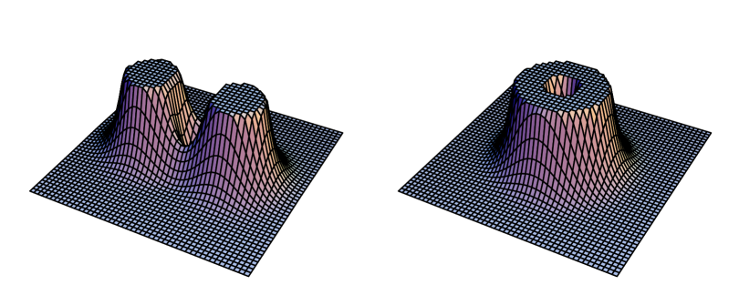
Figure 2: Wigner distributions for two coherent states placed at distances greater than (left) and less than (right) the lattice size $\propto\sqrt{\hbar}$.

The observations above lead to the conclusion that for a semiclassical observer, it makes sense to think of states as inhabiting a lattice of unit cell area $2\pi\hbar$ [23]. In fact a semiclassical observer measures the phase plane at an area scale $\delta A=2\pi\hbar M\gg 2\pi\hbar$. At this scale, the observer is only sensitive to a smooth, coarse grained Wigner distribution $0\leq\hbar W_{c}=u_{c}\leq 1$ which erases many details of the precise underlying precise microstates. We may view the region $\delta A$ as consisting of $M=\delta A/2\pi\hbar$ lattice sites, a fraction $u_{c}=\hbar W_{c}$ of which are occupied by coherent states. Then the entropy of the local region $\delta A$ is

$$S_{K}=\log{\binom{M}{\hbar\,W_{c}\,M}}\sim-M\log{(\hbar W_{c})^{\hbar W_{c}}(1-\hbar W_{c})^{1-\hbar W_{c}}}=-\frac{\delta A}{2\pi\hbar}\log{u_{c}^{u_{c}}(1-u_{c})^{1-u_{c}}}\,.$$ (45)

The Stirling approximation used in (45) is valid when $\hbar W_{c}$ is reasonably far from 0 and 1. For the total entropy this gives

$$S = \int dS=\int dA\,(\frac{dS}{dA})$$ (46)

$$\frac{dS}{dA} = -\frac{u_{c}\log{u_{c}}+(1-u_{c})\log{(1-u_{c})}}{2\pi\hbar}\,.$$ (47)

It is beautiful that thinking about $u_{c}=\hbar W_{c}$ as the probability of occupation of a site by a coherent state, this is simply Shannon’s formula for information in a probability distribution.

These facts imply that in the semiclassical limit the function $u(x_{1},x_{2})$ which completely defines a classical solution should effectively be defined on a lattice with each plaquette of area $\mathcal{O}(\hbar)\leftrightarrow\mathcal{O}(\ell_{P}^{4})$, and take values of 0 or 1 in each site. Likewise (47) will be interpreted as an expression for the entropy of arbitrary half-BPS asymptotically ${\rm AdS}_{5}\times S^{5}$ spacetimes. As an example it exactly reproduces the formula for the entropy of the typical states described in [10] that correspond in spacetime to the “superstar” geometry [22].

Note that the entropy vanishes if and only if $u$ equals $0$ or $1$ everywhere. Following the correspondence (9) such states map into geometries that are non-singular. We learn that semiclassical half-BPS geometries that are smooth all have vanishing entropy; and the presence of singularities $0<u<1$ also implies that the spacetime carries an entropy. Thus, in this setting, entropy is a measure of ignorance of a part of the underlying state which is captured in classical gravity as a spacetime singularity.

4.2 The partition function

In the semiclassical limit the partition function over the half-BPS sector of IIB string theory (${\cal M}$) with asymptotically ${\rm AdS}_{5}\times S^{5}$ boundary conditions can be written as

$$Z=\int_{{\cal M}}\mathcal{D}g_{\mu\nu}\cdots\,e^{-\beta(H(g_{\mu\nu},\cdots)-\gamma N(g_{\mu\nu},\cdots))}=\int\mathcal{D}u(x_{1},x_{2})\,\mu(u)\,e^{-\beta(H(u)-\mu N(u))}\,.$$ (48)

We are able to write this as a functional integral over just $u$ because the entire classical solution can be derived from this function, as can the Hamiltonian $H$ and the number of units of 5-form flux $N$. The measure $\mu(u)$ reflects not only the Jacobian in transforming between the supergravity fields and $u$, but also the number of underlying microscopic configurations that give rise to the same macroscopic spacetime. To derive the semiclassical measure $\mu$ recall first that the classical metric is a useful concept at scales $L\gg\ell_{P}$ and the semiclassical limit can be defined as (34). In this limit the smooth function $u(x_{1},x_{2})$ arises by considering the limit of piecewise constant functions in the lattice of scale $L$. To derive the continuum measure $\mu(u)$ we first ask how many microscopic configurations can give rise to a given average value of $u$ in each $L\times L$ lattice cell. From the previous section we have learned that we can think of $u$ as the average number of Planck size cells that are populated by coherent states within an area of size $L\times L$. Following (45) this means that a coarse-grained plaquette of size $L$ with a given value of $u$ arises from

$$\binom{L/\ell_{P}}{u\,L/\ell_{P}}$$ (49)

underlying configurations. Many of these configurations, representing different occupation numbers of Planck cells, will have different energies because the energy contribution of a given Planck cell depends upon its location as $E=(x_{1}^{2}+x_{2}^{2})/2$ (4). However, because $L\to 0$ in the semiclassical limit, configurations that populate a fixed fraction of Planck sized cells will necessarily have very similar energies. In fact it can be shown that the energies are even similar in Planck units in the strict semiclassical limit (34). This is because as $L/\ell_{P}\to\infty$, the number of Planck cells in each plaquette is extremely large. One can use this to show that the energies of configurations that populate a fixed fraction $u$ of the Planck cells have a standard deviation to mean ratio that vanishes as $L/\ell_{P}\to\infty$.

Putting everything together, the measure on semiclassical half-BPS spacetimes is

$$\mu(u)=e^{-\int{dx_{1}\,dx_{2}\over 2\pi\hbar}\,\left(u\ln{u}+(1-u)\ln(1-u)\right)}=e^{S(u)}$$ (50)

where $S$ is understood as the entropy of the spacetime. In the semiclassical limit, a spacetime is nonsingular if $u=0,1$ everywhere. In that case, $S(\mu)=0$ and the measure $\mu$ is 1. In other words, semiclassical half-BPS spacetimes have an entropy if and only if they are singular.

Defining

$$f(x_{1},x_{2})=\beta\left({x_{1}^{2}+x_{2}^{2}\over 4\pi\hbar}-{\mu\over 2\pi\hbar}\right)$$ (51)

the partition function over semiclassical half-BPS spacetimes becomes

$$Z=\int{\mathcal{D}}u(x_{1},x_{2})\,e^{-\int{dx_{1}\,dx_{2}\over 2\pi\hbar}\,\left[u\ln{u}+(1-u)\ln(1-u)+f\,u\right]}$$ (52)

Evaluating this by the method of saddlepoints gives

$$\ln Z=\int\frac{d^{2}x}{2\pi\hbar}\ln(1+e^{-\beta\frac{x_{1}^{2}+x_{2}^{2}}{2\hbar}+\beta\mu})=\int_{0}^{\infty}ds\,\frac{s}{e^{s-\beta\mu}+1}\equiv\frac{1}{\beta}F_{2}(e^{\beta\mu}),$$ (53)

where $s=\beta(x_{1}^{2}+x_{2}^{2})/2$ and $F_{2}$ is a Fermi-Dirac function. It is worth emphasizing that we have summed over both singular and non-singular semiclassical spacetimes, but have included the correct degeneracy factor (50). A naive approach to summing over geometries would have failed to include this measure because there is no semiclassical horizon giving arise to a Bekenstein-Hawking entropy. In such a a naive approach the partition function would have been

$$\ln\tilde{Z}=\int\frac{d^{2}x}{2\pi}\ln\left(\frac{1-e^{(-\beta\frac{x_{1}^{2}+x_{2}^{2}}{2}+\beta\mu)}}{\beta\frac{x_{1}^{2}+x_{2}^{2}}{2}-\beta\mu}\right)=\frac{1}{\beta}\int_{0}^{\infty}ds\ln\left(\frac{1-e^{-s-\beta\mu}}{s-\beta\mu}\right).$$ (54)

This integral diverges at the upper limit. A naive approach taking the unit measure over geometries would only reproduce (53) if we restricted the partition sum to be over smooth geometries ($u=0,1$) with $u$ taking constant values within elementary cells at the Planck scale. This would mimic in geometry the coherent state analysis given above, but its validity is more doubtful because at the Planck scale the wavefunction over geometries is always relevant.

The semiclassical partition function (53) should reproduce the partition function obtained from first principles by coarse-graining the scale of the fundamental cells in the quantum mechanical phase space. This procedure is not ambiguous because the free fermion gauge theory description provides us with an honest quantum mechanical phase space. Coarse-graining is defined as a renormalization group transformation in this space, and it is the 1/2 BPS nature of the quantum states that allows us to trust this description as the value of the coupling is turned on to achieve a reliable gravitational description. Consider then a lattice whose cells are $M\times M$ (in Planck units). From the microscopic point of view, the energy of each distribution of populated Planck scale cells is different, but as we argued before, in the limit $M\to\infty$, almost all distributions cluster close to a certain typical distribution in the $M\times M$ cell, and thus observers at these scales will assign the same energy to all of them. In this case, the coarse-grained function $u$ will take values $0,\frac{1}{M^{2}},\frac{2}{M^{2}},\ldots,1$ in the $M\times M$ cells. This can also be seen from the flux quantization (5) which is scale independent. In other words, discretising phase space and comparing two lattices of sizes $M\times M$ and $1\times 1$, in Planck units, we find that

$$N=\sum_{\{x_{1},\,x_{2}\}}u(x_{1},\,x_{2})=M^{2}\,\sum_{\{x_{1}^{M},\,x_{2}^{M}\}}u^{M}(x_{1}^{M},\,x_{2}^{M})\,\,\,\Rightarrow\,\,\,u^{M}(x_{1}^{M},\,x_{2}^{M})=\frac{1}{M^{2}}\,\!\!\!\!\sum_{\stackrel{{\scriptstyle\{x_{1},\,x_{2}\}}}{{\in\{x_{1}^{M},\,x_{2}^{M}\}}}}\!\!\!\!u(x_{1},\,x_{2})\,,$$ (55)

where variables with superscript $M$ are defined in the $M\times M$ lattice and in the second equality we are summing over all Planck-scale lattice sites inside a single $M\times M$ cell labelled by $(x_{1}^{M},\,x_{2}^{M})$. This sum computes the fraction of populated sites in the coarse-grained cell. Finally, the sum over $u^{M}$ at cell location $(x_{1}^{M},x_{2}^{M})$ becomes

$$\sum_{u^{M}}e^{-f\,u^{M}}=1+\binom{M^{2}}{1}e^{-f\frac{1}{M^{2}}}+\binom{M^{2}}{2}e^{-f\frac{2}{M^{2}}}+\ldots+\binom{M^{2}}{M^{2}}e^{-f\frac{M^{2}}{M^{2}}}=\left(1+e^{\frac{-f}{M^{2}}}\right)^{M^{2}}.$$ (56)

The factors in front of each exponential count how many ways a given value of $u^{M}$ in the coarse-grained lattice can be attained in terms of the Planck scale lattice. The complete partition function becomes

$$Z^{M\times M}=\prod_{x_{1},x_{2}\in M\mathbb{Z}}\left(1+e^{-\frac{\beta}{M^{2}}(\frac{x_{1}^{2}+x_{2}^{2}}{2}-\mu)}\right)^{M^{2}}=\frac{M^{2}}{\beta}F_{2}(e^{\frac{\beta\mu}{M^{2}}})\,.$$ (57)

Thus, coarse-graining the phase space lattice size rescales the temperature, i.e. $T\to T\,M^{2}$. This derivation reproduces the semiclassical computation if we identify the temperature $\beta$ in (53) as the rescaled one. We could view the computation (57) as a derivation for the entropy formula (45).

5 The microscopic origin of macroscopic moments

In the previous section we computed the partition function over the $\frac{1}{2}$-BPS sector, fixing the energy $E$ and the five-form flux $N$ using Lagrange multipliers $\beta,\,\mu$. In this section, we shall analyse other interesting ensembles in which different charges are fixed in the same way.

5.1 Fixing the integrable charges

The typical states of fixed energy have a spectrum of the charges $M_{k}$ defined in (11) that is fixed by the universal $u$ function that describes their classical limit [10]. However, it is clear that classical spacetimes with different angular moments are easily constructed by varying the radial dependence of the $u$ function. Hence it is of interest to ask what spacetime gives the universal classical description of the typical state with fixed moments $M_{k}$. We can also use the measure (50) on half-BPS spacetimes to find out how many classically indistinguishable microstates are described by the same metric. We also see that classical spacetimes with atypical macroscopic moments are exponentially unlikely in the space of all states.

A natural way to identify typical states carrying fixed values of these charges is to analyze ensembles of states that generalize the grand-canonical one by introducing as many chemical potentials $\mu_{k}$ as conserved charges $M_{k}$ we want to fix. As usual, we will fix the values of these charges by requiring the expected values to match our desired value, a step that determines the set of chemical potentials.

While it is technically difficult to achieve this description in the basis of states provided by the Young tableaux, it is very natural in the coherent state basis. Indeed, the semiclassical expressions (11) are linear in the phase space density $u_{0}$, and so they are straightforward to integrate in the path integral that defines the semiclassical partition function:

$$Z=\int\mathcal{D}u(x_{1},x_{2})\,\mu(u)\,e^{-\beta(H(u)-\mu N(u))}\,e^{-\mu_{k}\,M_{k}}\equiv\mathcal{D}u(x_{1},x_{2})\,\mu(u)\,e^{-\sum_{i=0}^{N}\mu_{i}\,M_{i}}\,.$$ (58)

Above we used $M_{0}=N$ and $M_{1}=E$ and relabelled their chemical potentials to reduce the notation. Using the measure (50) and evaluating the partition function by the method of saddlepoints, its logarithm becomes

$$\ln Z^{M_{i}}=\int_{0}^{\infty}dx\frac{\sum_{i}i\mu_{i}x^{i}}{e^{\sum_{i}\mu_{i}x^{i}}+1}\,,$$ (59)

which is a natural extension of the usual Fermi–Dirac statistics. The value of the phase space density $u$ is fixed by the saddlepoint:

$$u=\frac{1}{1+e^{-\sum_{i=0}^{N}\mu_{i}\,M_{i}}}\,.$$ (60)

In this ensemble it is trivial to find an expression for the expected moments; it is simply

$$\bar{M}_{n}=-\partial_{\mu_{n}}\ln Z.$$ (61)

5.2 Moments in the $(x_{1},x_{2})$ plane

The eigenstates of the $M_{k}$ (11) that were considered above have phase space densities that are rotationally invariant in the phase space and thus correspond to $u$ functions that are rotationally invariant in the $x_{1},\,x_{2}$ plane. In particular, any half-BPS state whose single particle phase space density is not rotationally invariant cannot be an eigenstate of the Hamiltonian. Density functions $u$ with angular dependence can be efficiently parameterized by expanding them in a Fourier series:

$$u(r,\phi)=u_{0}(r)+\sum_{p=1}^{\infty}u_{p}^{c}(r)\cos p\phi+\sum_{p=1}^{\infty}u_{p}^{s}(r)\sin p\phi\,.$$ (62)

To work out the kinds of states which give rise to $u$ functions with $u^{c}_{p},u^{s}_{p}\neq 0$ we work with the Young tableaux basis of states, and consider superpositions of the form:

$$\Psi(\vec{q})=\sum_{w}c_{w}\Psi^{\mathcal{F}^{w}}(\vec{q})\,.$$ (63)

Above, $w$ indexes the basis states in the superposition, each given as a Slater determinant of single particle states as $\Psi^{\mathcal{F}^{w}}(\vec{q})=\frac{1}{\sqrt{N!}}\det(\psi_{f^{w}_{i}}(q_{j}))$, and $\mathcal{F}^{w}$ is the set of excitation numbers characterizing the basis state $\Psi^{\mathcal{F}^{w}}(\vec{q})$. The normalization is such that $\sum_{w}|c_{w}|^{2}=1$. The states (63) are $N$ particle states, whereas the phase space density $W$ which is mapped onto the spacetime data $u$ (9) is a one particle density.

The method for calculating the one-particle Wigner density function is given in [10] (also see Appendix A). Using this, it is easy to show that because the wavefunctions $\psi_{f_{i}}(q_{j})$ are orthogonal, the only interference terms between various pieces of the superposition (63) that survive involve states $w$ and $w^{\prime}$ having $N-1$ of the fermion excitations in $\mathcal{F}^{w}$ and $\mathcal{F}^{w^{\prime}}$ equal. Let us denote by $\mathcal{C}$ the set of pairs of states of this kind. For each pair define the differing excitation $a_{(w,w^{\prime})}$ by $\{a_{(w,w^{\prime})}\}=\mathcal{F}^{w}\backslash\mathcal{F}^{w^{\prime}}$. With this definition we can now compute the one particle Wigner distribution corresponding to (63)

$$W(q,p) = \int\frac{dy}{\hbar}\rho_{1}(q-y,q+y)e^{\frac{2ipy}{\hbar}}=\frac{2\,e^{-\frac{r^{2}}{\hbar}}}{\hbar}\sum_{w}|c_{w}|^{2}\sum_{f\in\mathcal{F}^{w}}(-1)^{f}L_{f}(\frac{2r^{2}}{\hbar})$$ (64)

$$+ \frac{2\,e^{-\frac{r^{2}}{\hbar}}}{\hbar}\sum_{\begin{subarray}{c}(w,w^{\prime})\in\mathcal{C}\\ m<n\end{subarray}}(-1)^{N_{m}+N_{n}}(-1)^{m}2^{\frac{n-m}{2}+1}\sqrt{\frac{m!}{n!}}\left(\frac{r}{\sqrt{\hbar}}\right)^{n-m}L_{m}^{n-m}(\frac{2r^{2}}{\hbar})$$

$$\times\left(\textrm{Re}\left\{c_{w^{\prime}}c^{*}_{w}\right\}\cos(n-m)\phi+\textrm{Im}\left\{c_{w^{\prime}}c^{*}_{w}\right\}\sin(n-m)\phi\right).$$

The shorthand notation $n=a_{(w,w^{\prime})}$ and $m=a_{(w^{\prime},w)}$ was used above for the sake of clarity. We also defined $N_{n}$ to index the number of the differing excitation, i.e. if $n=a_{(w,w^{\prime})}=f_{i}^{w}\in\mathcal{F}^{w}$, then $N_{n}\equiv i$.

Eq. (64) illustrates how interference between Young tableau basis states in the superposition (63) is responsible for breaking the $\textrm{U}(1)$ invariance in the $y=0$ plane, i.e. all $\phi$ dependence in $u(r,\phi)$ is due to interference between basis states. To quantify this, we match the Fourier components of (62) with those of (64) giving

$$u_{0}(r) = 2e^{-\frac{r^{2}}{\hbar}}\sum_{w=1}^{M}|c_{w}|^{2}\sum_{f\in\mathcal{F}^{w}}(-1)^{f}L_{f}(\frac{2r^{2}}{\hbar}),$$

$$u_{p}^{c}(r) = 2e^{-\frac{r^{2}}{\hbar}}\sum_{\begin{subarray}{c}(w,w^{\prime})\in\mathcal{C}\\ n-m=p\end{subarray}}(-1)^{N_{m}+N_{n}}(-1)^{m}2^{\frac{p}{2}+1}\sqrt{\frac{m!}{n!}}L_{m}^{p}(\frac{2r^{2}}{\hbar})\left(\frac{r}{\sqrt{\hbar}}\right)^{p}\textrm{Re}(c_{w^{\prime}}c^{*}_{w}),$$ (65)

$$u_{p}^{s}(r) = 2e^{-\frac{r^{2}}{\hbar}}\sum_{\begin{subarray}{c}(w,w^{\prime})\in\mathcal{C}\\ n-m=p\end{subarray}}(-1)^{N_{m}+N_{n}}(-1)^{m}2^{\frac{p}{2}+1}\sqrt{\frac{m!}{n!}}L_{m}^{p}(\frac{2r^{2}}{\hbar})\left(\frac{r}{\sqrt{\hbar}}\right)^{p}\textrm{Im}(c_{w^{\prime}}c^{*}_{w}).$$ (66)

This shows that we have a simple relation between the fourier modes of $u$ and the states in the superposition: a given mode $u_{p}^{c,s}(r)$ arises from interference between basis states that share $(N-1)$ of their excitations, but differ by $p$ units in the remaining excitation. Thus the energy difference between the two states is $p\hbar$.

While the above shows that breaking of $U(1)$ invariance in the $y=0$ plane necessarily arises from interference in a Young tableau basis, we should also recall that the geometric description is only valid if we have an approximate eigenstate of the metric operator. We have seen in Sec. 4 that any given Wigner distribution can be constructed out of coherent states for the fermions and that such a state will be a eigenstate of the metric operator. Such states can also be written as complicated superpositions in a Young tableau basis.

We would like to identify what typical states correspond to which violations, and count how many of them there are. This is again difficult to achieve in the Young tableaux basis, but it is straightforward in the coherent state basis by introducing the appropriate Lagrange multipliers fixing the appropriate charges.

To quantify the angular moments, define the quantities

$$\mathcal{U}_{p}^{c}\equiv\int\frac{d^{2}r}{2\pi}u(r,\phi)\cos p\phi=\frac{1}{2}\int_{0}^{\infty}dr\ ru_{p}^{c}(r)\,,\quad p>0,$$ (67)

with a similar expression for $\mathcal{U}_{p}^{s}$. Note that for $p=0$ the corresponding quantity is just the flux of the five-form field, $\int_{0}^{\infty}dr\,r\,u_{0}(r)=N$.

With this definition we can construct the ensemble by introducing Lagrange multipliers $\alpha_{p}^{c}$ and $\alpha_{p}^{s}$ as

$$e^{-\beta(E-\mu N)+\sum_{p=1}^{\infty}(\alpha_{p}^{c}\mathcal{U}_{p}^{c}+\alpha_{p}^{s}\mathcal{U}_{p}^{s})},$$ (68)

from which we can again compute the partition function to be

$$Z_{\mathcal{U}}=\prod_{x_{1},x_{2}}\left(1+e^{-\beta(\frac{r^{2}}{2}-\mu)+\sum_{p=1}^{\infty}(\alpha_{p}^{c}\cos p\phi+\alpha_{p}^{s}\sin p\phi)}\right).$$ (69)

The logarithm can again be computed

$$\ln Z_{\mathcal{U}} = \frac{1}{2\pi\beta}\int_{0}^{\infty}\int_{0}^{2\pi}\frac{x}{e^{-\beta\mu-\sum_{p=1}^{\infty}(\alpha_{p}^{c}\cos p\phi+\alpha_{p}^{s}\sin p\phi)}e^{x}+1}$$ (70)

$$= \frac{1}{2\pi\beta}\int_{0}^{2\pi}F_{2}(e^{\beta\mu+\sum_{p=1}^{\infty}(\alpha_{p}^{c}\cos p\phi+\alpha_{p}^{s}\sin p\phi)})\,d\phi.$$

Thus we see that fixing the fourier modes $\mathcal{U}_{p}$ is very natural in this language, though the integrals are again difficult to compute and we are no longer working with Fermi–Dirac statistics.

Exponential suppression of moments:

We shall now show that the number of states with non-zero moments $\mathcal{U}^{c,s}$ is exponentially smaller than the number of states with $\mathcal{U}^{c,s}=0$. To show this, we shall fix one of the moments, chosen to be $\mathcal{U}_{p}^{c}\equiv\mathcal{U}$, and consider the density matrix of this ensemble: $\hat{\rho}=\frac{1}{Z}e^{-\beta(\hat{E}-\mu\hat{N})+\alpha\hat{\mathcal{U}}}$. From this it follows that the entropy is

$$S_{\alpha}=-\langle\ln\hat{\rho}\rangle=\ln Z+\beta E-\beta\mu N-\alpha\mathcal{U},$$ (71)

where the partition funtion is given by (70), and $E,N$ and $\mathcal{U}$ are determined in the standard way by differentiating the partition function with respect to the Lagrange multipliers:

$$E = T^{2}\partial_{T}\ln Z+T\mu\partial_{\mu}\ln Z=\frac{1}{2\pi\beta^{2}}\int_{0}^{2\pi}F_{2}(e^{\beta\mu+\alpha\cos p\phi})\,d\phi,$$

$$N = T\partial_{\mu}\ln Z=\frac{1}{2\pi\beta}\int_{0}^{2\pi}F_{1}(e^{\beta\mu+\alpha\cos p\phi})\,d\phi,$$

$$\mathcal{U} = \partial_{\alpha}\ln Z=\frac{1}{2\pi\beta}\int_{0}^{2\pi}\cos p\phi\ F_{1}(e^{\beta\mu+\alpha\cos p\phi})\,d\phi.$$ (72)

Analyzing these relations exactly is complicated and we need to specify a regime of parameters in which to work. To produce macroscopic angular moment, we choose to work with states of high energy or equivalently with a low density of fermions. This corresponds to working in the limit $\mu\to-\infty$, such that $e^{\beta\mu\pm\alpha}\to 0$. In this limit the Fermi–Dirac functions can be approximated by $F_{n}(e^{\beta\mu\pm\alpha})\approx e^{\beta\mu\pm\alpha}$, and the relations (72) simplify considerably.

The remaining integrals in (72) can be computed using the calculus of residues, and after a short computation they yield

$$\ln Z \approx N\approx\beta E\approx\frac{e^{\beta\mu}}{\beta}\sum_{n=0}^{\infty}\frac{1}{n!^{2}}\left(\frac{\alpha}{2}\right)^{2n},$$

$$\mathcal{U} \approx \frac{e^{\beta\mu}}{\beta}\sum_{n=0}^{\infty}\frac{1}{n!(n+1)!}\left(\frac{\alpha}{2}\right)^{2n+1}.$$ (73)

To invert these relations let us choose the Lagrange multiplier $\alpha$ to be very small, which will correspond to choosing the moment to be small, but still macroscopic and measurable. Truncating the sums to their first two terms, we can invert the relations above to give

$$\beta=\frac{N}{E} \equiv \frac{1}{xN},$$

$$\mu=-\frac{E}{N}\ln[\frac{E}{N^{2}}(1+\frac{\mathcal{U}}{N}^{2})] \equiv -xN\ln[x(1+a^{2})],$$

$$\alpha=2\frac{\mathcal{U}}{N} \equiv 2a,$$ (74)

where we have defined the scalings $E=xN^{2}$ and $\mathcal{U}=aN$. Note that the assumption of high energy requires large $x$, which immediately results in $\beta\mu\ll-1$, which is consistent with our assumption. Also, the angular moment is still measurable, since it scales linearly with $N$, with $\alpha$ small but fixed.

Inserting these relations into (71) we get

$$S_{\alpha}=N(\ln x+2)-N(\frac{2a^{2}}{1+a^{2}}-\ln(1+a^{2})),$$ (75)

which shows that the number of states with macroscopic moments of size $aN$ is exponentially suppressed from the rotationally invariant case:

$$\frac{e^{S_{a}}}{e^{S_{a=0}}}=e^{-N(\frac{2a^{2}}{1+a^{2}}-\ln(1+a^{2}))}.$$ (76)

Variances:

Since fixing the macroscopic moment exponentially reduces the number of available states, it is necessary to check that the fluctuations in the previous computation are not so large as to render the computation invalid. The spread in the expectation value of $\mathcal{U}$ is given by the standard deviation to mean ratio, which can be computed to give

$$\frac{\sigma(\mathcal{U})}{\langle\mathcal{U}\rangle}=\sqrt{\frac{\langle\mathcal{U}^{2}\rangle-\langle\mathcal{U}\rangle^{2}}{\langle\mathcal{U}\rangle^{2}}}=\sqrt{\frac{\frac{\partial_{\alpha}^{2}Z}{Z}-\left(\frac{\partial_{\alpha}Z}{Z}\right)^{2}}{\left(\frac{\partial_{\alpha}^{2}Z}{Z}\right)^{2}}}\approx\frac{1}{a\sqrt{2N}},$$ (77)

where the computation was carried out in the previous high energy regime, using the relations (73). This vanishes as $N\to\infty$, and therefore this ensemble is statistically valid.

Measurability of interference:

Just as eigenstates of the Hamiltonian generate non-trivial higher conserved charges at infinity, we can ask whether the presence of angular moments in the $(x_{1},\,x_{2})$ plane, arising from interference between Young tableau components in the superposition (63), has any characteristic effect asymptotically. In [21] we analysed how the integrable charges $M_{k}$ associated to Young tableau states appear at different orders in an asymptotic expansion of $u$, the function determining the metric. For the question at hand the same method turns out to be very cumbersome, as the Young tableaux basis is not a convenient one to use when analysing the moments in the $x_{1},x_{2}$ plane. For completeness, we still include the asymptotic expansion analogous to (12) for the superposition state (63):

$$u(\rho,\theta,\varphi) = 2\cos^{2}\theta\sum_{l=0}^{\infty}\frac{\hbar^{l+1}\sum_{w}|c_{w}|^{2}2^{l}\langle M_{l}^{\mathcal{F}^{w}}\rangle}{\rho^{2l+s}}(-1)^{l}(l+1)\,\,{{}_{2}F_{1}}(-l,l+2,1;\sin^{2}\theta)$$ (78)

$$+ 4\cos^{2}\theta\sum_{l=1}^{\infty}\frac{(-1)^{l}\hbar^{\frac{l}{2}+1}}{\rho^{l+2}}\sum_{i=[\frac{l}{2}]+1}^{l}(-1)^{i}(i+1)\sin^{2i-l}\theta\sum_{p=0}^{[i-\frac{l+1}{2}]}2^{\frac{l}{2}+p-i}$$

$$\times\binom{i}{2i-l}\binom{2i-l}{p}\sum_{\begin{subarray}{c}(w,w^{\prime})\in\mathcal{C}\\ n-m=2(i-p)-l\end{subarray}}(-1)^{N_{m}+N_{n}}\sqrt{\frac{n!}{m!}}\textrm{Re}(c_{m}^{*}c_{n}e^{i(n-m)\phi})$$

$$\times\left(\frac{d}{da}\right)^{l-i+p}\left[a^{i-p}(a-1)^{m}\right]_{a=2}.$$

The first row of this expansion is a weighted sum of the single state contributions of (12), while the last three rows arise from interference between the states in the superposition. As one might imagine, analysing interference directly from this expression would be very complicated, but we want to point out that all odd powers of $\frac{1}{\rho}$ in the expansion come from the interference terms. Thus, if an asymptotic observer measures such a moment, she could infere that the underlying quantum state necessarily was in a linear superposition of Young tableaux.

To examine whether these moments are semiclassically measurable, it is more convenient to work with the coherent state picture of section (4.1). Using coherent states we can engineer any moments $\mathcal{U}^{c,s}_{p}$ we wish, by distributing the fermions in a suitable way. As an example, let us pick a very specific configuration with exactly one $U(1)$ violating moment turned on:

$$u(r,\phi)=\frac{1}{2}\Theta(\sqrt{2}R^{2}-r)(1+2a\cos\phi),$$ (79)

where $\Theta$ is the Heaviside step function, $a$ is a parameter controlling the size of $U(1)$-violation and $R=(2\hbar N)^{\frac{1}{4}}$ is the AdS radius. One sees that for this distibution $\mathcal{U}_{1}^{c}=aN$, and therefore for small $a$ the state is of the form analyzed earlier in this section.

An asymptotic expansion of the function $u(\rho,\theta,\phi)$ corresponding to this fermion distribution can be computed via the technique used in [21], and the first non-trivial terms turn out to be

$$u(\rho,\theta,\phi)=\frac{\cos^{2}\theta}{\rho^{2}}\hbar N+\frac{2^{\frac{5}{2}}a}{3}\frac{\cos^{2}\theta\sin\theta\cos\phi}{\rho^{3}}(\hbar N)^{\frac{3}{2}}+\mathcal{O}(\rho^{-4})\,.$$ (80)

The $(\hbar N)^{3/2}$ dependence of the first odd $\rho$ negative power illustrates the finiteness of this moment in the semiclassical limit:

$$N\to\infty,\quad\hbar\to 0,\quad\textrm{ such that }\hbar N=\textrm{ fixed}.$$ (81)

Thus, the interference between the Young tableau components of some states is measurable by an asymptotic observer, even though for a typical state these effects are highly suppressed as shown in (76).

6 $N\rightarrow 1$-particle information loss

Our work above has emphasized that individual quantum states do not generically correspond to individual geometries. In particular, we have shown how a geometry arising from a specified function $u(x_{1},x_{2})$ as in (3) can be the effective coarse-grained description of many quantum states. As noted in section 3.3, the function $u$ determines only the expectation value of the (coarse-grained) operator $\tilde{u}$. Furthermore, this function encodes only information present in the one-particle phase space density [10, 21] derived by projection of the full quantum state. Below, we first characterize more precisely when this projection loses information. It will turn out that in the semiclassical limit, the 1-particle projection loses information if and only if the description as an LLM geometry is singular. We then characterize the operators which probe beyond this one-particle projection from several points of view. (See [10] for a discussion of related issues.)

6.1 Singularities and loss of information

In Sec. 3.1 we gave four examples of states that give rise to single particle phase space distributions that reproduce the metric of the ‘superstar’ extremal black hole. Two of these states, “Square + Square” (15) and “Triangle + Triangle” (14), have identical single particle distributions even though they are very different as $N$-particle states. In this case, the “Square + Square” state does not have a description as a single geometry since it is not an approximate eigenstate of the metric operator. But it is easy to devise examples of multiple states, all of which have good descriptions as a single coarse-grained geometry, and which have identical single particle phase space distributions. The projection to the single particle phase space has lost information about the underlying $N$-particle configurations.

To see when this situation may occur, suppose that the support of the function $u$ on the $(x_{1},x_{2})$ plane has an area $2\pi\hbar k$. As in section 4.1, we envision the fermions as coherent states inhabiting a lattice, and identify the support of $u$ with lattice sites $\{\lambda_{1},\ldots,\lambda_{k}\}={\rm supp}\,u$. Also, because there are $N$ fermions, we must have

$$\int\frac{dx_{1}dx_{2}}{2\pi\hbar}\,u=N\,.$$ (82)

Thus, the wavefunction is a sum of $N$-particle components, each of which is of the form $|\lambda_{i_{1}},\ldots,\lambda_{i_{N}}\rangle$, where $i_{s}\in{\rm supp}\,u~{}~{}\forall s$. There are $\binom{k}{N}$ such $N$-particle components, so the superposition coefficients required to specify the general state involve $2\binom{k}{N}-2$ real numbers (where we subtract $2$ to account for the normalization and the unphysical overall phase). On the other hand, since the Wigner distribution is nonzero at $k$ lattice sites, it contains $k-1$ real numbers (after accounting for the normalization (82)). Therefore, when $k>N$, the 1-particle projection simply does not contain enough data to determine the underlying $N$-particle state.

In any situation where the effective phase space distribution has support on more than $N$ lattice sites, the normalization (82) will force the distribution to take values that are neither $0$ nor $1$ in at least some locations. In that case, following the correspondence (9), the spacetime geometry is necessarily singular. Since the density takes values other than $0$ or $1$, we see that the fine-grained metric also fluctuates; our state is not an approximate eigenstate of the fine-grained $\hat{u}$. In this sense then, singularities in the half-BPS sector of ${\rm AdS}_{5}$ gravity arise precisely when a single classical geometry is unable to encode some data concerning the underlying quantum mechanical configuration space. This is satisfactory because any attempt to do physics in these singular spacetimes forces us to specify boundary conditions on the singularity. As mentioned in [10], it would be very interesting to understand how these boundary conditions emerge from the effect of coarse-graining of wave functions applied to correlation functions in the gauge theory.

6.2 Operators probing $N$-particle structure

Second-quantized formalism:

The second-quantized formalism of section 3.2 makes it particularly easy to exhibit operators sensitive to more than 1-particle structure. We simply string together creation and annihilation operators corresponding to different sites on the LLM plane. One example is

$$\hat{\mathcal{O}}_{10}=b^{\dagger}(1)b(1)b^{\dagger}(0)b(0)\,,$$ (83)

where $b(0)$ stands for the second-quantized operator that destroys a particle in the $0^{{\rm th}}$ level in the energy eigenbasis. Then:

$$\begin{array}[]{lcl}\hat{\mathcal{O}}_{10}|\textrm{`triangle + triangle'}\rangle&=&0\\ \hat{\mathcal{O}}_{10}|\textrm{`square + square'}\rangle&=&\frac{1}{\sqrt{2}}|0,1,\ldots,N-1\rangle\end{array}$$ (84)

where the two states above are specified in (15,14). Here the ‘square + square’ state does not have a good description as a single geometry, but we could have equally given an example where the $N$-particle distinguished two states that have both have good descriptions in an identical geometry.

Wigner’s formalism:

Recall that the expectation value of a 1-particle operator $\hat{\mathcal{O}}$ in a state represented by the 1-particle reduced Wigner distribution $W_{1}(\alpha,\alpha^{*})$ is

$$\langle\hat{\mathcal{O}}\rangle=\frac{\hbar}{\pi}\int_{\mathbb{C}}d^{2}\alpha f_{\mathcal{O}}(\alpha,\alpha^{*})W_{1}(\alpha,\alpha^{*})\,,$$ (85)

where $f_{\mathcal{O}}(\alpha,\alpha^{*})$ is the classical phase space distribution corresponding to $\hat{\mathcal{O}}$. The formalism of Wigner distributions extends to calculating expectation values of operators sensitive to multi-particle structure. The $N$-particle Wigner distribution is given by:

$$W_{N}(\vec{q},\vec{p})=\hbar^{-N}\int_{-\infty}^{\infty}d\vec{y}\langle\vec{q}-\vec{y}|\hat{\rho}_{N}|\vec{q}+\vec{y}\rangle\,e^{2i\vec{p}\cdot\vec{y}/\hbar}\,.$$ (86)

From this, the 1-particle reduced Wigner distribution is recovered by tracing over $N-1$ particles:

$$W(\alpha,\alpha^{*})=\frac{N\,\hbar^{N-1}}{\pi^{N-1}}\int d^{2}\alpha_{2}\ldots d^{2}\alpha_{N}W_{N}(\vec{\alpha},\vec{\alpha}^{*})\,.$$ (87)

In analogy to the 1-particle case, expectation values of operators in states characterized by $W_{N}$ are given by:

$$\langle\hat{\mathcal{O}}\rangle=\frac{\hbar^{N}}{\pi^{N}}\int_{\mathbb{C}^{N}}d^{2N}\vec{\alpha}f_{\mathcal{O}}(\vec{\alpha},\vec{\alpha}^{*})W_{N}(\alpha,\alpha^{*})\,.$$ (88)

Note that $f_{\mathcal{O}}(\vec{\alpha},\vec{\alpha}^{*})$ is necessarily symmetric in the $\alpha_{i}$’s.

From the above, it is clear that operators admitting a representation $\mathcal{O}(\vec{\alpha},\vec{\alpha}^{*})=\sum_{i}f(\alpha_{i},\alpha_{i}^{*})$ can be completely evaluated in the 1-particle reduced Wigner distribution:

$$\langle\hat{\mathcal{O}}\rangle = \frac{\hbar^{N}}{\pi^{N}}\int_{\mathbb{C}^{N}}d^{2N}\vec{\alpha}\textrm{ }W_{N}(\vec{\alpha},\vec{\alpha}^{*})\sum_{i}f(\alpha_{i},\alpha_{i}^{*})$$

$$= \frac{\hbar}{\pi}\sum_{i}\int_{\mathbb{C}}d^{2}\alpha_{i}f(\alpha_{i},\alpha_{i}^{*})\left(\frac{\hbar^{N-1}}{\pi^{N-1}}\int_{\mathbb{C}^{N-1}}\prod_{j\not{=}i}d^{2}\alpha_{j}W_{N}(\vec{\alpha},\vec{\alpha}^{*})\right)$$

$$= \frac{\hbar}{\pi}\sum_{i}\int_{\mathbb{C}}d^{2}\alpha_{i}f(\alpha_{i},\alpha_{i}^{*})\left(\frac{1}{N}W_{1}(\alpha_{i},\alpha_{i}^{*})\right)$$

$$= \frac{\hbar}{\pi}\int_{\mathbb{C}}d^{2}\alpha f(\alpha,\alpha^{*})W_{1}(\alpha,\alpha^{*})\,.$$

On the other hand, any operator whose classical density is not of the form $\sum_{i}f(\alpha_{i},\alpha_{i}^{*})$ (i.e. contains a monomial in $\alpha$’s of mixed indices) will generically probe the $N$-particle structure. The space of 1-particle operators with non-vanishing expectation values admits a basis given by the moments $M_{n}$ (10) with classical phase space densities

$$\mathcal{O}_{n}=\sum_{i}(\alpha_{i}\alpha_{i}^{*})^{n}=M_{n}\,.$$ (89)

This is intuitive as the knowledge of all the $M_{n}$’s is in principle necessary and sufficient for specifying $W_{1}$. Any operator which is not a linear combination of the $M_{n}$’s will in general probe the $N$-particle information.

$N$-particle operators in full AdS/CFT:

The recognition of 1-particle operators as the higher Hamiltonians of the fermionic system afford a clean characterization of operators probing the $N$-particle structure in the full CFT. In particular, any operator which may not be written as a linear combination of $\hat{\mathcal{O}}_{n}=\textrm{Tr}\,(X^{\dagger n}X^{n})$ will belong to this family. $R$-charge conservation and gauge invariance translates this requirement into the following: operators probing the $N$-particle structure are multi-trace operators. Not surprisingly, multi-trace operators correspond to multi-particle states on the gravity side [24]. They have been investigated in [25, 26]. A simple example of such an operator is

$$\textrm{Tr}\,(X^{\dagger}X)\,\textrm{Tr}\,(X^{\dagger}X)-\textrm{Tr}\,(X^{\dagger 2}X^{2})\,,$$ (90)

where the second term removes the 1-particle component. Its classical phase space distribution is given by

$$\{\,|\alpha_{1}|^{2}|\alpha_{2}|^{2}\,\}\,,$$ (91)

where $\{\ldots\}$ denotes complete symmetrization over $\alpha_{1},\ldots,\alpha_{N}$.

7 Discussion

Our definition of the metric operator $\hat{u}(x_{1},x_{2})$ was based on the use of standard coherent states, having equal dispersions in $x_{1}$ and $x_{2}$. Similarly, our notion of coarse-graining was based on Gaussian smearing kernels having equal $x_{1}$- and $x_{2}$-dispersions. This choice was made for the sake of simplicity and, furthermore, for an observer who makes sufficiently rough measurements (i.e., who is sufficiently semi-classical) of a fixed state, the detailed shape of $\hbar$-sized phase space cells is irrelevant. However, consider a given “semi-classical” observer who is able to measure energies with some fixed accuracy $\delta E$. Suppose that this observer studies one of the above coherent states centered on a point with $r^{2}=x_{1}^{2}+x_{2}^{2}$. This state has an energy uncertainty $\Delta E\sim r\delta r/\hbar\sim r/\sqrt{\hbar}$. Clearly for large $r$ we have $\Delta E\gg\delta E$ and the observer’s measurements will cause this state to quickly decohere.

Such measurements are not well-described by our formalism above. Instead, such observers require an analogous formalism based on squeezed coherent states, where the squeezing reduces the radial dispersion to achieve $\delta r\sim\hbar/r$ at the expense of increasing the angular dispersion to the level $\delta\theta\sim 1$, such that $r\delta r\delta\theta\sim\hbar$. They also require a correspondingly squeezed notion of coarse graining. It would be very interesting to study such a squeezed formalism in detail, but we have chosen the simpler (unsqueezed) formalism for our work above. It would also be interesting to analyze bulk semi-classical observers from first principles to verify that fixed energy resolution $\delta E$ (as opposed to a $\delta E$ which changes with $E$) is in fact an appropriate description of their measurements.

Appendix A Computing the Wigner distribution

In this appendix we present the computation of the Wigner distribution for a general state in the $N$-particle harmonic oscillator, deriving (64). A general state can be written as a superposition of basis states as (63), and the single particle wavefunctions appearing in the Slater determinant are given by

$$\psi_{f}(q)=(\pi\hbar)^{-\frac{1}{4}}\frac{e^{-\frac{q^{2}}{2\hbar}}}{\sqrt{2^{f}f!}}H_{f}(\frac{q}{\sqrt{\hbar}}),$$ (92)

where $H_{n}$ is a Hermite polynomial. We then compute the effective one particle density matrix as

$$\rho_{1}(x,y) = \int dq_{2}\ldots dq_{N}\Psi^{*}(x,q_{2},\ldots,q_{N})\Psi(y,q_{2},\ldots,q_{N})$$ (93)

$$= \int dq_{2}\ldots dq_{N}\sum_{w,\tilde{w}}c_{w}^{*}c_{\tilde{w}}\epsilon^{i_{1}\ldots i_{N}}\epsilon^{1j_{2}\ldots j_{N}}\epsilon^{k_{1}\ldots k_{N}}\cdot$$

$$\cdot\epsilon^{1l_{2}\ldots l_{N}}\psi^{*}_{f_{i_{1}}^{w}}(x)\psi^{*}_{f_{i_{2}}^{w}}(q_{j_{2}})\ldots\psi^{*}_{f_{i_{N}}^{w}}(q_{j_{N}})\psi_{f_{k_{1}}^{\tilde{w}}}(y)\psi_{f_{k_{2}}^{\tilde{w}}}(q_{l_{2}})\ldots\psi_{f_{k_{N}}^{\tilde{w}}}(q_{l_{N}})$$

$$= \ldots=\sum_{w=1}^{M}\left(|c_{w}|^{2}\sum_{f\in\mathcal{F}^{w}}\psi^{*}_{f}(x)\psi_{f}(y)\right)$$

$$+\sum_{(w,\tilde{w})\in\mathcal{C}}(-1)^{N_{(w,\tilde{w})}+N_{(\tilde{w},w)}}c^{*}_{w}c_{\tilde{w}}\psi^{*}_{a_{(w,\tilde{w})}}(x)\psi_{a_{(\tilde{w},w)}}(y).$$

Before explaining the notation above, some comments are in order. The right hand side of (93) consists of two parts. The ‘diagonal’ terms on the upper line are contributions of single basis states, as already computed in [10], only now weighted by $|c_{w}|^{2}$. The second part, the ‘cross terms’, represent interference between basis states. Due to the orthogonality of the 1-particle wavefunctions (92) it is clear that a cross term between two basis states appears if $(N-1)$ of the excitations in these states are the same, i.e. the sets $\{f_{1}^{w},\ldots,f_{N}^{w}\}$ and $\{f_{1}^{w^{\prime}},\ldots,f_{N}^{w^{\prime}}\}$ have $(N-1)$ equal elements, while the remaining elements differ. Note that when this happens, the crossed basis states necessarily have different energies and the superposition state is prohibited from being a hamiltonian eigenstate.

The notation is as follows: let $\mathcal{C}$ denote the set of pairs that give rise to interference terms as explained above. Then for each excitation we can define the differing excitation $a_{(w,w^{\prime})}$ as $\{a_{(w,w^{\prime})}\}\in\mathcal{F}^{w}\backslash\mathcal{F}^{w^{\prime}}$. We also define the index of the differing excitation such that if $a_{(w,w^{\prime})}=f_{i}^{w}\in\mathcal{F}^{w}$, then $N_{(w,w^{\prime})}=i$.

The Wigner distribution corresponding to a density matrix $\hat{\rho}_{1}$ is defined as

$$W(q,p)=\frac{2}{\hbar}\int_{-\infty}^{\infty}dy\,\langle q-y|\hat{\rho}_{1}|q+y\rangle\,\,e^{\frac{2ipy}{\hbar}},$$ (94)

and using equations (92), (93) and the identity

$$\int_{-\infty}^{\infty}dxe^{-x^{2}}H_{m}(x+y)H_{n}(x+z)=2^{n}\sqrt{\pi}m!z^{n-m}L_{m}^{n-m}(-2yz),\quad m\leq n,$$ (95)

it is now straightforward to verify (64). Above the $L_{a}^{b}$ are associated Laguerre polynomials.

References

- [1]
- [2] H. Lin, O. Lunin and J. Maldacena, “Bubbling AdS space and 1/2 BPS geometries,” JHEP 0410, 025 (2004) [arXiv:hep-th/0409174].
- [3]
- [4] V. Balasubramanian, M. Berkooz, A. Naqvi and M. J. Strassler, “Giant gravitons in conformal field theory,” JHEP 0204, 034 (2002) [arXiv:hep-th/0107119].
- [5]
- [6] S. Corley, A. Jevicki and S. Ramgoolam, “Exact correlators of giant gravitons from dual N = 4 SYM theory,” Adv. Theor. Math. Phys. 5, 809 (2002) [arXiv:hep-th/0111222].
- [7]
- [8] D. Berenstein, “A toy model for the AdS/CFT correspondence,” JHEP 0407, 018 (2004) [arXiv:hep-th/0403110].
- [9]
- [10] V. Balasubramanian, J. de Boer, V. Jejjala and J. Simon,“The Library of Babel: On the origin of gravitational thermodynamics”, JHEP 0512, 006 (2005) [arXiv:hep-th/0508023].
- [11]
- [12] L. F. Alday, J. de Boer and I. Messamah, “The gravitational description of coarse grained microstates,” JHEP 0612, 063 (2006) [arXiv:hep-th/0607222].
- [13]
- [14] K. Larjo, “On the existence of supergravity duals to D1–D5 CFT states,” arXiv:hep-th/0705.4433.
- [15]
- [16] L. D’Errico, W. Muck and R. Pettorino, “Stretched Horizon and Entropy of Superstars,” arXiv:hep-th/0703223.
- [17]
- [18] H.-H. Shieh, G. van Anders, M. Van Raamsdonk, “Coarse-Graining the Lin-Maldacena Geometries,” arXiv:hep-th/0705.4308.
- [19] G. Milanesi and M. O’Loughlin, “Singularities and closed time-like curves in type IIB 1/2 BPS geometries,” JHEP 0509, 008 (2005) [arXiv:hep-th/0507056].
- [20] M. Hillery, R.F. O’Connell, M.O. Scully and E.P. Wigner, “Distribution functions in physics: fundamentals”, Physics Reports 106, No. 3, (1984) 121-167.
- [21] V. Balasubramanian, B. Czech, K. Larjo and J. Simon, “Integrability vs. information loss: A simple example,” JHEP 0611, 001 (2006) arXiv:hep-th/0602263.
- [22] R. C. Myers and O. Tafjord, “Superstars and giant gravitons,” JHEP 0111, 009 (2001) [arXiv:hep-th/0109127].
- [23] V. Bargmann, P. Butera, L. Girardello and J. R. Klauder, “On The Completeness Of The Coherent States,” Rept. Math. Phys. 2, 221 (1971); A. M. Perelomov, Teor. Mat. Fiz. 6, 213 (1971)’ H. Bacry, A. Grossmann and J. Zak, “Proof of completeness of lattice states in the k q representation,” Phys. Rev. B 12, 1118 (1975).
- [24] O. Aharony, M. Berkooz and E. Silverstein, “Multiple-trace operators and non-local string theories,” JHEP 0108, 006 (2001) [arXiv:hep-th/0105309], “Non-local string theories on AdS(3) x S**3 and stable non-supersymmetric backgrounds,” Phys. Rev. D 65, 106007 (2002) [arXiv:hep-th/0112178].
- [25] E. Witten, “Multi-trace operators, boundary conditions, and AdS/CFT correspondence,” arXiv:hep-th/0112258.
- [26] M. Berkooz, A. Sever and A. Shomer, “Double-trace deformations, boundary conditions and spacetime singularities,” JHEP 0205, 034 (2002) [arXiv:hep-th/0112264].