Structure and Dynamics of the Sun’s Open Magnetic Field

Abstract

The solar magnetic field is the primary agent that drives solar activity and couples the Sun to the Heliosphere. Although the details of this coupling depend on the quantitative properties of the field, many important aspects of the corona - solar wind connection can be understood by considering only the general topological properties of those regions on the Sun where the field extends from the photosphere out to interplanetary space, the so-called open field regions that are usually observed as coronal holes. From the simple assumptions that underlie the standard quasi-steady corona-wind theoretical models, and that are likely to hold for the Sun, as well, we derive two conjectures on the possible structure and dynamics of coronal holes: (1) Coronal holes are unique in that every unipolar region on the photosphere can contain at most one coronal hole. (2) Coronal holes of nested polarity regions must themselves be nested. Magnetic reconnection plays the central role in enforcing these constraints on the field topology. From these conjectures we derive additional properties for the topology of open field regions, and propose several observational predictions for both the slowly varying and transient corona/solar wind.

1 Introduction

Decades of solar XUV/X-ray observations have shown that the Sun’s corona is divided into two distinct types of magnetic regions: those in which field lines are “closed”, i.e., rooted to the photosphere at two ends, and those in which field lines are “open”, rooted to the photosphere at only one end and extending out to the Heliosphere. The fast solar wind is believed to emanate from these open field regions, which usually appear dark in X-rays and, therefore, are referred to as coronal holes. Although a great deal of progress has been made on understanding the Sun’s open magnetic field since the seminal work of Parker (1958), many questions remain outstanding, especially concerning the dynamics of solar-heliospheric coupling. For example, we still do not understand the magnetic topology and evolution that give rise to the slow wind (e.g., Axford & McKenzie, 1997; Zurbuchen, 2007). At an even more basic level, the coronal and heliospheric observations themselves appear to be in conflict. Coronal images often show streamer evolution and inflows/outflows that are interpreted as closed flux opening into the wind and open flux closing back down to the streamer (Hundhausen et al., 1984; Howard et al., 1985; Sheeley & Wang, 2002). Furthermore, the long-standing observation that some coronal holes appear to rotate rigidly, impervious to differential rotation (Timothy et al, 1975; Zirker, 1977), implies the continuous opening and closing of coronal field (Wang, Hawley, & Sheeley, 1996; Lionello et al., 2006). However, the opening of closed flux implies the injection of field lines into the wind with both footpoints connected to the photosphere. Such field lines should exhibit a bi-directional heat flux (counter-streaming electrons) in heliospheric measurements, yet counter-streaming electrons are rarely seen outside of interplanetary coronal mass ejections (ICMEs) (Gosling, 1990). Conversely, the closing down of open flux would imply the formation of U-shaped field lines in the heliosphere with no connection to the Sun, resulting in a heat flux drop-out in the heliospheric measurements (McComas et al., 1989, 1991; Lin & Kahler, 1992). Again, these are rarely seen outside of ICMEs (Pagel, Crooker, & Larson, 2005). Apparently, the heliosphere does not care what the corona is doing!

This apparent contradiction among the observations has led to conflicting approaches to modeling the topology and evolution of the open field. Motivated by their observations, some heliospheric researchers have proposed the interchange model, in which reconnection between open and closed flux is the dominant process by which the coronal open field evolves (Fisk, Zurbuchen, & Schwadron, 1999; Fisk, 2005; Fisk & Zurbuchen, 2006). Note that reconnection between an open and a closed field line produces another pair of open and closed field lines, and no disconnected lines (Crooker, Larson, & Kahler, 2002). In this model the magnetic topology is presumed to be highly complex, with open field mixing into closed field regions as in a diffusion process.

On the other hand, motivated by their observations solar researchers have primarily used the quasi-steady model in which the coronal magnetic field is calculated from the instantaneous normal component at the photosphere using some extrapolation procedure. The simplest and most widely-used such procedure is the source surface model, in which the field is assumed to be current-free in the corona and to be purely radial at some fixed spherical surface (Altschuler & Newkirk, 1969; Schatten, Wilcox, & Ness, 1969; Hoeksema, 1991). This model predicts a topology consisting of distinct open flux (coronal holes) and closed flux regions (Wang & Sheeley, 1990; Arge & Pizzo, 2000; Luhmann et al., 2002, 2003; Schrijver & DeRosa, 2003). Although the dynamics are not explicitly calculated, field-line opening and closing driven by the evolution of the photospheric flux are implicit in this model. The assumption is that the coronal field evolution can be approximated by a sequence of source-surface solutions. The quasi-steady models have been extended in recent years to include solution of the full MHD equations, no longer requiring the assumption of a current-free magnetic field in the corona and an artificial source surface. Typically, the MHD models are used to compute a steady-state equilibrium (e.g., Linker et al., 1999; Riley, Linker, & Mikic, 2001; Odstrcil, 2003; Roussev et al., 2003), but they can also be employed for fully dynamic simulations (Riley et al., 2003).

It should be emphasized that the quasi-steady models are nothing more than particular implementations of Parker’s basic theory of the solar wind. In his seminal work, Parker (1958) argued that if the gas pressure in the corona becomes larger than the magnetic pressure, the gas must expand outward as a wind, dragging the field lines with it. Hence, the open and closed regions are fundamentally determined by the magnitude of coronal heating and the magnitude of the field in the corona. Implicit in Parker’s theory is the assumption that field will open and close in response to changes in these quantities. In principle, the MHD models are a more physical representation of the theory; but since the coronal heating mechanism is not known, they are also ad hoc in practice.

Although the interchange and quasi-steady models predict very different topology and dynamics of the open field, they both agree that reconnection is the dominant physical process involved in the opening and closing of magnetic flux. Reconnection is also the process generally invoked for transient opening and closing of flux by CMEs (see reviews by Forbes, 2000; Klimchuk, 2001; Low, 2001; Wu, Andrews, & Plunkett, 2001; Linker et al., 2003; Lin, Soon, & Baliunas, 2003). In this paper we adopt the solar-centric view that the coronal field is given by some straightforward extrapolation of the photospheric boundary conditions, such as a source-surface or MHD solution. Using two straightforward assumptions and some analytic arguments, we derive strict constraints on the open-field topologies allowed by the quasi-steady models. We also discuss the central role of reconnection in determining coronal hole structure and dynamics.

2 Basic Assumptions of the Quasi-Steady Model

The first assumption is that all rapidly varying, small-scale structure in the photospheric field, such as the clumping into elementary flux tubes (Solanki, 1993; Muller, 1994) and the so-called magnetic carpet (Schrijver et al., 1997), can be neglected when calculating the topology of the open field. It should be emphasized that, given sufficient numerical resolution, the quasi-steady models can incorporate arbitrary spatial structure in the photospheric flux distribution. The influence of the small-scale photospheric structure generally disappears at heights far below the source surface; but, if desired, one could always include this spatial structure in the model. The problem, however, is that the small-scale structure may not be compatible with the assumption of quasi-steady evolution. Since both the magnetic field and the wind must reach a steady state, the quasi-steady assumption requires an evolution slow compared to either a sound or Alfven crossing time of the corona. Hence for a typical sound speed of $\sim 10^{7}$ cm/s and scale of order the solar radius $\sim 10^{11}$ cm, the restriction is that the photospheric field evolves on the time scale of hours or longer.

This restriction holds for fields of the scale of active regions, but not for the small magnetic-carpet bipoles. The effect of these small temporal and spatial scale bipoles is to add some high-frequency “noise” to the system. The interchange advocates would argue that it is exactly this “noise” that is responsible for the distinguishing feature of their model: open field can diffuse freely into closed field regions. It seems unlikely, however, that the small-scale carpet fields can have such a dramatic effect on the field topology. The key point is that, even in the presence of the magnetic carpet, the structure of the coronal field is determined by the balance between the Lorentz force and gas pressure. This means that, in the low-beta corona where the field dominates, the time-averaged field line geometry must resemble that of a fully closed potential or, more generally, a force-free-equilibrium field. Note that this constraint holds even in the open field regions. Field lines can deviate significantly from the potential/force-free state only at heights where the gas pressure becomes of order the magnetic pressure. Therefore, in those regions where the force-free field lines never reach large heights, the field must be closed irrespective of any “noise” due to the presence of the carpet. The occurrence of open field lines in such a region would require a large deviation from the geometry of the force-free state, which would violate basic force balance.

The second assumption of the quasi-steady model is that there are no long-lived current sheets in the closed field corona. (In this paper we use the term “current sheet” to refer exclusively to a true discontinuity in the field, not to merely a large concentration of electric current.) This second assumption is also likely to be valid, because the corona is low beta and appears to be evolving slowly (except during CMEs and flares), so the field must be in a fairly robust equilibrium. It has been argued by several authors that current sheets are not likely to exist in the force-free corona (van Ballegooijen, 1985; Antiochos, 1987). Note that the small-scale, transient currents required by many models of coronal heating (e.g., Parker, 1983) are allowed, but are not expected to influence the global corona. Furthermore, long-lived volumetric currents such as those induced by photospheric shearing and twisting motions are also allowed and can be arbitrarily large, as long as there are no true discontinuities in the magnetic field. Of course in the source surface models there are no currents whatsoever, the field is assumed to be potential, but volumetric currents are almost certain to be present in the MHD models.

3 Coronal Hole Uniqueness

Although the assumptions of smooth currents and a quasi-steady corona seem innocuous, they actually place severe restrictions on coronal hole topology. In particular, we claim that they imply the following “uniqueness conjecture”:
Every unipolar region on the photosphere can contain at most one coronal hole.

We do not have a rigorous mathematical proof of this conjecture that holds for all possible topologies; instead, we present below compelling arguments that it should hold for observed solar conditions, as long as the assumptions above are valid. In particular, it should hold for the quasi-steady, source-surface and MHD models. We believe, however, that the conjecture is valid in general.

3.1 Bipolar Topology

To clarify our arguments for uniqueness, consider first the simplest possible coronal topology: a bipolar field with one coronal hole in each unipolar region. An analytic source-surface solution for such a field can be obtained by using the method of images (Jackson, 1962). For a dipole $\vec{d}$ located at a point $\vec{r_{d}}$ inside the Sun, and a source surface at radius $R_{S}$, the magnetic field potential, $\vec{B}=-\nabla\Phi$ is given by:

$$\Phi=\frac{\vec{d}\cdot(\vec{r}-\vec{r_{d}})}{|\vec{r}-\vec{r_{d}}|^{3}}-\frac{R_{S}r_{d}^{3}\vec{d}\cdot(R_{S}^{2}\vec{r}-r^{2}\vec{r_{d}})}{|r_{d}^{2}\vec{r}-R_{S}^{2}\vec{r_{d}}|^{3}}.$$ (1)

It is straightforward to verify that $\Phi=0$ at the source surface, $r=R_{S}$, so the field is purely radial there. Equation (1) is highly useful, because one can build up a field of arbitrary complexity simply by adding more dipoles. For the simplest possible case of a single dipole at Sun center pointed along the vertical axis, Equation (1) reduces to:

$$\Phi=\frac{(\vec{d}\cdot\vec{r})({R_{S}}^{3}-r^{3})}{{R_{S}}^{3}r^{3}}$$ (2)

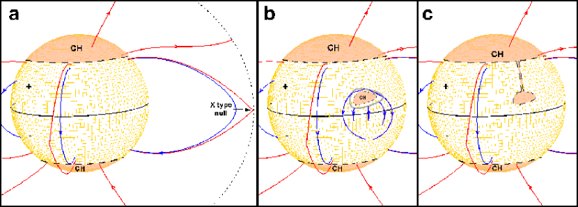
Figure 1: (a) Source-surface solution for a bipolar coronal field with two coronal holes indicated by the darker areas. The solid black line denotes the PIL at the equator, while the dashed black lines indicate the boundaries of the coronal holes. Red and blue solid lines denote open and closed field lines, respectively. (b) A hypothetical disconnected coronal hole is drawn in the northern hemisphere of (a). An example of an annulus of closed flux surrounding one of the holes is shown in grey, with hypothetical field lines that close across the equator in blue. (c) An example of an open field corridor connecting the coronal holes of panel (b).

and is shown in Figure 1a for $R_{S}=2.5$ with the solar radius normalized to unity.

Topologically, the magnetic field can be considered to define a mapping that connects the points along any field line in the volume. This mapping is given by integrating the equations for a field line:

$$\frac{dx}{ds}=\frac{B_{x}}{B},\quad\frac{dy}{ds}=\frac{B_{y}}{B},\quad{\rm and}\quad\frac{dz}{ds}=\frac{B_{z}}{B},$$ (3)

where $s$ is distance along a field line and $x,y$, and $z$ are the coordinates of the field line at the point $s$. It is apparent from these formulas that, in order for the mapping to be discontinuous, i.e., for field lines to“split”, either one of the components $B_{x},B_{y}$, or $B_{z}$, must be discontinuous, which implies the presence of a singularity in the current (a current sheet), or the magnitude $B$ must vanish. All the arguments below follow from this straightforward, but very powerful result: In the absence of singular currents, magnetic field lines can split only at locations where the field vanishes, such as true null points. Although we will use this result only in the context of solar coronal magnetic fields, we emphasize that it holds in general. For example, the classical model for the magnetosphere, a dipole embedded in a background field, exhibits the topological feature that the field lines split only at the magnetopause and distant-tail null points (Cowley, 1973; Stern, 1973; Lau & Finn, 1990).

Note that the field of Fig. 1a does vanish at the null line located on the equator of the source surface and, in fact, the field lines do split there. (For a source surface solution the null is of the X-type, whereas for a solution with a solar wind it would be of the Y-type; but this difference is irrelevant to our argument.) Equations 1 - 3 confirm our expectation that the mapping must be discontinuous across a coronal-hole boundary. This boundary is a true separatrix surface, just like the well-known fan surface described below. However the mapping defined by Equation (2) is continuous everywhere else, in particular, in the closed field region. Since there are no currents in the closed field corona of Fig. 1a, the field line mapping is especially simple; but, even if photospheric flows were applied that greatly deformed the polarity distribution and that generated strong current in the corona, the field line mapping would remain continuous as long as the flows were smooth (Antiochos, 1987). Note that we allow for the possibility of quasi-separatrix layers (QSL), where the mapping exhibits large gradients (Titov, Hornig, & Demoulin, 2002) as long as it is not truly discontinuous.

The key point in the argument for uniqueness is that the field lines in the closed-field region of Fig. 1a cannot split, because neither of the necessary conditions is met: a simple bipolar region contains no nulls and, by assumption, no current sheets are present there. If the field lines cannot split, it is straightforward to demonstrate that the positive and negative polarity regions of Fig. 1a can each contain only one coronal hole. Assume that a second disconnected hole exists, for example, in the northern hemisphere, (Fig. 1b). This second hole must be fully inside the northern polarity region, because as a direct consequence of the absence of current sheets:
A coronal hole boundary cannot intersect a polarity inversion line (PIL).
This condition must be generally valid, otherwise the heliospheric current sheet would extend all the way down to the photosphere, violating our fundamental assumptions. (Note that to avoid confusion with magnetic null lines, we will use the more-precise term PIL rather than the term “photospheric neutral line” that is also commonly used.) Since the coronal holes do not intersect each other or the PIL, there must exist an annulus of flux in the closed region that completely encircles one of the holes but not the other, as sketched in Fig. 1b. This annulus flux must map to a negative region across the equatorial PIL. Because the open flux of the coronal holes constitutes a barrier that extends to infinity, it is evident from Fig. 1b that the flux of any such annulus must go around at least one of the coronal holes in order to connect across the PIL; i.e., the field lines must split in the closed corona region. But this is not possible in the absence of current sheets; hence, a second disconnected coronal hole is forbidden.

This simple but compelling argument implies several important points. If open field is intermixed with the closed field, as in the interchange model, the topology is equivalent to many small coronal holes embedded in the larger scale closed field. Therefore, by reversing our argument, we conclude that the interchange model requires the presence of many current sheets in the corona. Furthermore, the current sheets must be inherently transient, because unlike the quasi-steady heliospheric current sheet, gas pressure cannot maintain current sheets in the low-beta corona.

3.2 Open Field Corridors

Another important point is that the coronal hole topology of Fig 1b requires only minor modification to make it agree with the uniqueness hypothesis: the addition of a very thin corridor of open field connecting the two holes, as illustrated in Fig. 1c. The geometry of the corridor can be arbitrary as long as it connects the holes, in which case it becomes impossible to find an annulus of closed field that passes between the two holes, and field-line splitting is no longer an issue. If the holes are connected, however, only one continuous coronal hole exists in the northern hemisphere, and uniqueness still holds. Note, however, that the corridor may be below observable resolution limits, so that the corona would appear to contain two disconnected holes, reconciling observations with our hypothesis. We contend that such narrow open-field corridors are likely to be present in the real corona, providing a natural explanation for the well-observed phenomenon of seemingly disconnected coronal holes (Kahler & Hudson, 2002).

It is easy to find open-field corridors in the source surface models of observed solar fields. Figure 2a shows the flux distribution for Carrington rotation 1922, and 2b shows the regions of open and closed field as calculated by the standard source surface model for this flux distribution. Although the polarity regions and the PILs are much more complex than the single dipole of Fig 1, both systems exhibit one dominant polarity in the north and one in the south with a PIL separating them. There are also numerous small opposite-polarity regions with their PILs separating them from the main polarities, but none of these appears to contain a coronal hole. It should be noted that the actual flux distribution at the photosphere used to calculate the source surface model of Fig. 2b contains many more opposite polarity regions than can be seen in Fig. 2a, which for ease of viewing, shows the flux slightly above the photosphere. These opposite polarity regions are responsible for the numerous, small closed-field circular regions near the boundary of the coronal hole in Fig. 2b. In fact, there are undoubtedly many more such regions throughout the polar coronal holes on the Sun than can be observed with present instrumentation, so a true coronal hole map must actually resemble a “swiss cheese” pattern. We will consider the effect of such opposite polarity regions later in this paper.

In the northern hemisphere near the center of Fig. 2b, the arrow points to a coronal hole that appears to be well separated from the main polar hole, but still in the same polarity region. If so, this would clearly violate uniqueness. In order to investigate this “disconnected” hole in detail, we calculate an analytic approximation to the field of Fig. 2a. Note that for Fig. 2a the solution was calculated numerically on a fixed grid using a finite-difference scheme to solve Laplace’s equation:

$$\nabla^{2}\Phi=0,$$ (4)

with $\Phi=0$ at the source surface. A finite-difference solution of Equation (4) is convenient for deriving initial conditions to a time-dependent code, but for examining the detailed topological properties of the source-surface model, a numerical solution is not as effective as an analytic one. Therefore, we have taken the magnetic flux distribution of Fig. 2a and calculated its spherical harmonic expansion out to large order $l=51$. Of course, a finite order expansion does not return the identical flux distribution on the boundary as in Fig. 2a, but this is not significant. Our only requirement is that the flux distribution be approximated sufficiently accurately that the “disconnected” hole is preserved.

Given the coefficients for the boundary-flux expansion, $C_{lm}$, we can then write down the exact source-surface solution in the domain (e.g., Wang & Sheeley, 1992),

$$\Phi=\sum_{l=1}^{L}\sum_{m=-l}^{l}C_{lm}\frac{Y_{lm}(\theta,\phi)}{r^{l+1}}\frac{(r^{2l+1}-R_{s}^{2l+1})}{(l+(l+1)R_{s}^{2l+1})},$$ (5)

where, as in Equation (2), the solar radius is normalized to unity. The advantage of this formulation is that, in principle, we can use the analytic solution given by Equation (5) to determine the field line mapping with arbitrary accuracy. (In practice, however, the computational time required may be prohibitive.) The other important advantage of the expansion above is that simply by using different values for the order of the expansion, $L$, we can investigate the effect of applying different levels of smoothing to the photospheric flux distribution.

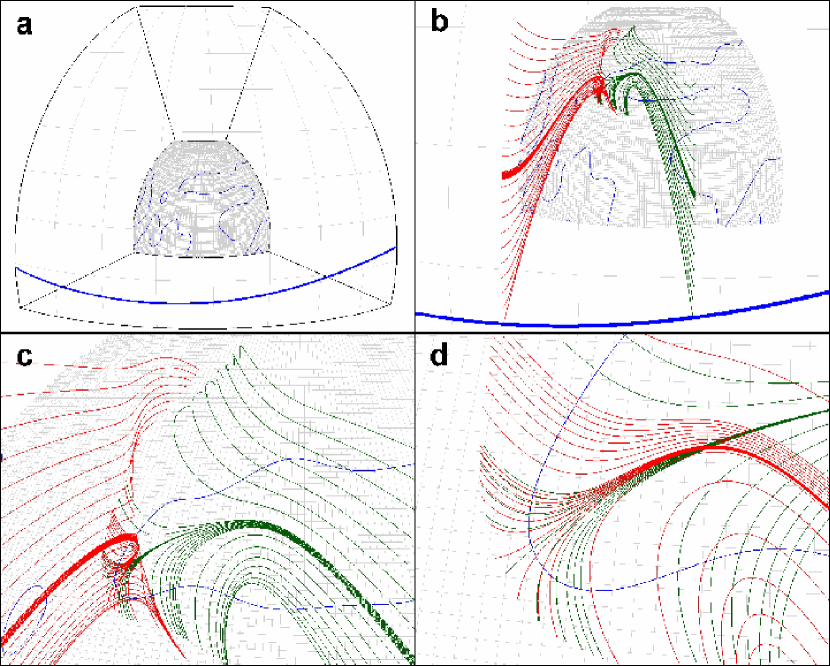
Figure 3: (a) Plotting domain for a spherical harmonic expansion solution with $L=31$. The blue contours correspond to the PILs on the photosphere and on the source surface. (b) Sets of field lines (red and green lines) traced from lines of constant longitude on the source surface down to the photosphere. (c) View of the photospheric footpoint positions of the field lines of the previous panel. (d) A close-up of the region near the tip of the negative polarity tongue showing that the footpoints of the red and green field lines become unresolvably close in this region.

We find that, for spherical harmonic solutions with order ranging up to $L=51$, all of the detailed open field structure evident in Fig. 2b disappears except for the “disconnected” hole in the north. Evidently, this hole is a robust feature of the photospheric polarity distribution. Fig. 3 presents results from the $L=31$ solution. The first panel (Fig. 3a) shows the domain used for plotting, along with the PIL on the photosphere (thin blue line) and the PIL on the source surface (thick blue line). The photospheric polarity is predominantly positive in the region shown, the north pole is all positive, but near the center of the region, there is an extended tongue of negative polarity oriented east-west. The “disconnected” hole of Fig. 2b lies south of this negative tongue. The next panel (Fig. 3b) shows two sets of open field lines (red and green) traced from the source surface down to the photosphere. The starting footpoints for the two sets are two lines of constant longitude separated by approximately $20^{\circ}$ in longitude on the source surface. Each set begins with a field line whose starting point is very close to the source surface PIL and whose end point on the photosphere lies in the “disconnected” hole, south of the negative polarity tongue. It is evident from Fig 3b that the field maps a line of constant longitude on the source surface to a line on the photosphere that passes from the small “disconnected” hole, around the tongue and into the main northern polar hole.

If the small hole were truly disconnected, then the field-line mapping would be discontinuous, and the line on the photosphere defined by each field-line set would contain a break. Figs 3c and 3d show closer views, (and from different perspectives), of the field line mapping at the photosphere. We note that the mapping is continuous, but as it passes around the tongue-like PIL, the mapping develops very large gradients there. We had to increase the density of starting footpoints on the source surface by two orders of magnitude in order to find field lines that map to locations near the tip of the tongue. For expansions of significantly higher order, such as $L=41$, the negative polarity tongue becomes more extended, and the mapping develops such large gradients that it becomes impossible with our numerical integration routine to find open field lines near the tip of the tongue by tracing downward from the source surface. To find such field lines one needs to begin the trace near the photosphere. This region of the field-line mapping can be considered to be an extreme example of a QSL. The key point, however, is that the field-line mapping is indeed continuous for all values of $L$, implying that a narrow corridor of open field must connect the southern hole to the main polar hole. Consequently, there is only one hole per unipolar region, in agreement with uniqueness.

As calculated from the spherical harmonic solution with $L=31$, the corridor has extremely narrow photospheric width, of order only 10 km at some locations. Note that the photospheric footpoints of the two field line sets are indistiguishable in Fig 3d, whereas the source-surface footpoints are separated by scales of order the solar radius. Such a small scale for the corridor width calls into question the quasi-steady assumption. A corridor of this scale on the Sun would be highly dynamic with field constantly opening and closing in response to small changes in the photospheric flux. But as long as the seemingly disconnected hole is present, then on average, a continuous corridor must exist. Note that additional, wider corridors can clearly be seen in the upper left of Fig. 2b. If enough corridors are present, then on a large scale the open and closed field will appear to be intermixed, so that near the coronal hole boundary the structure of the quasi-steady models may begin to resemble that of the interchange model. Furthermore, since they are likely to be continually dynamic the corridors could become an important source of the slow wind. This issue clearly needs further study.

3.3 Multipolar Topology

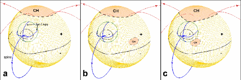
Figure 4: (a) Source-surface solution for a bipolar active region embedded in the global dipole of Fig. 1. For clarity, the southern coronal hole is not shown. A 3D null occurs at the point of intersection of all the blue field lines. The blue line closing into the negative south is the outer spine; the line closing into the negative spot is the inner spine. The other 4 lines lie on the fan surface. The green dotted line indicates the separatrix curve, the intersection of the photosphere and the fan surface. (b) A disconnected coronal hole in the topology of panel (a) that is forbidden by the annulus argument. (c) A hypothetical topology in which the nested-polarity separatrix curve intersects the two coronal holes, thereby circumventing the annulus argument and contradicting uniqueness.

The argument above was developed for a simple bipolar magnetic topology. The real corona, as seen in Fig. 2, usually contains other large-scale structures, such as active regions. These add topological complexity to the coronal field, especially null points where field lines do split. Therefore, the next step in the proof for uniqueness is to consider the effect on the arguments above of adding an active-region bipole to the topology of Figure 1. If the active region merely distorts the equatorial PIL, as in the well-studied case of May 12, 1997 (Arge et al., 2004), the topology of the closed field is still bipolar, and the annulus argument above holds. Similarly, if the active region emerges inside one of the open field regions, then the only effect is to produce a small closed-field region inside one of the polar holes, which again has no effect on the topology of the main closed region or on our argument. A significant change in topology occurs only if the active region produces a new PIL in the closed field photosphere, as in the field of Fig. 4a, where we have added a new low-latitude dipole source to Eq. (1). The potential is now given by:

$$\Phi=\Phi_{0}+\frac{\vec{d_{1}}\cdot\vec{r}}{|\vec{r}-\vec{r_{1}}|^{3}}-\frac{R_{S}^{3}r_{1}^{3}\vec{d_{1}}\cdot\vec{r}}{|r_{1}^{2}\vec{r}-R_{S}^{2}\vec{r_{1}}|^{3}},$$ (6)

where $\Phi_{0}$ is the potential of Equation (2), $\vec{d_{1}}=(0,A,0)$, and $\vec{r_{1}}=(.9,60^{\circ},0)$. In other words, a dipole pointing due north is placed at a latitude of $30^{\circ}$ and a depth of $0.1R_{\odot}$.

The addition of the active-region dipole produces a new PIL separating the negative active-region spot from its positive surroundings. We will use the term nested polarity region to refer to a configuration like the negative spot, which is wholly surrounded by a larger opposite-polarity region. The fact that some of the surroundings are in the form of a strong positive spot just south of the strong negative spot is not important to the topology. Associated with the active-region PIL is a null point in the corona, along with the usual dome-shaped fan separatrix surface and pair of spine lines (e.g., Greene, 1988; Lau & Finn, 1990; Antiochos, 1990; Priest & Titov, 1996). The intersection of the fan with the photosphere forms a closed separatrix curve defining the boundary between the positive flux connecting across the active-region PIL and that connecting across the equatorial PIL. Note that the field lines of the fan and spines all connect to the null and split there; consequently, the mapping is discontinuous at the fan and spines. The magnetic field of Fig. 4a is simply the well-known embedded bipole, the most likely topology if there are two PILs (three polarity regions) on the photosphere (Antiochos, 1998).

The only other possible topology for a two-PIL photosphere is that of a “bald patch” in which the null point occurs below the surface and the magnetic field over part of the nested PIL is concave up (e.g., Titov, Priest, & Demoulin, 1993). Bald patch topologies can occur only if the nested polarity region is small; therefore, they are unlikely to play a significant role in determining the large-scale solar field, such as the coronal hole topology. On the other hand, they have interesting implications for coronal dynamics, because we do not expect bald patch topologies to survive in open field regions (Antiochos & Mueller 2007 in preparation). Determining the evolution of bald patch topologies is problematic, however, because simple line-tied boundary conditions cannot be used wherever the coronal field is concave up at the photosphere (Antiochos, 1990; Karpen, Antiochos, & DeVore, 1990). Consequently, we will not consider bald patch topologies further in this paper.

It should be emphasized that the null-point topology of Fig. 4a is observed to be a generic feature of coronal magnetic fields. It was immediately seen by Skylab, where it was referred to as a “fountain” region (Tousey et al., 1973; Sheeley et al., 1975), and by Yohkoh where it was referred to as an “anemone” region (Shibata et al., 1994; Vourlidas et al., 1996). As demonstrated by numerous extrapolations of observed photospheric fields, it is ubiquitous throughout the Sun on a broad range of scales (e.g., Aulanier et al., 2000; Fletcher et al., 2001; Luhmann et al., 2003; Ugarte-Urra, Warren, & Winebarger, 2007). Of course, the true solar field is almost always more complex than that of a single active-region bipole. However, if the photospheric flux consisted of clearly separated embedded bipoles, each with its own PIL, then the topology would simply be that of a collection of non-intersecting fans and spines. Even for complex active regions, we expect that such regions also appear mainly bipolar, on the large scale that is important for determining the global field. Therefore, if uniqueness holds for the topology of Fig. 4a, it is likely to hold in general for all observed solar fields.

We now add a disconnected coronal hole to the system shown in Fig. 4a, and consider the implications of the null-point topology for our uniqueness conjecture. If the separatrix curve of the nested polarity does not intersect a coronal hole boundary as in Fig. 4b, then it is always possible to find an annulus of closed flux surrounding either hole that maps across the equatorial PIL. In this case the presence of the nested polarity is irrelevant, and the field of the annulus must split around one of the holes, which is disallowed. Thus, our earlier argument for uniqueness applies without change. But what happens if the active region moves or expands, such that its associated separatrix curve intersects the coronal holes as sketched in Fig. 4c? In this case there is no annulus of flux closing across the equator that encircles only one of the holes – all such annuli encircle both holes, so that no splitting of the field is required. Furthermore, any annulus of closed flux that encircles only one of the holes must cross the nested-polarity separatrix curve, in which case the annulus flux is allowed to split at the null point.

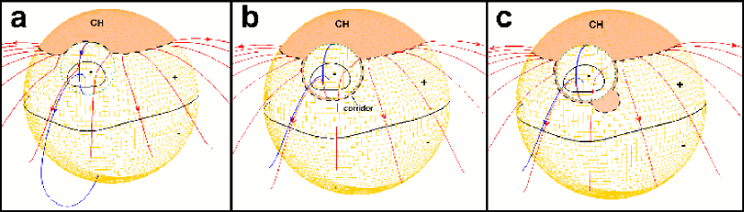
Figure 5: (a) Source-surface solution as in Fig. 4a, but for an active region dipole that is further north. (b) The source-surface solution for the dipole moved just $1^{\circ}$ north from (a). The outer spine is now open and the coronal hole boundary completely surrounds the nested polarity region. An open-field corridor separates the closed nested-polarity flux from the closed global flux. (c) The correct topology for the system of Fig. 4c.

Although a rigorous treatment of the topology implied by Fig. 4c requires a fully dynamic calculation, we can gain useful insight by considering the topology predicted by a sequence of static models in which a nested-polarity separatrix curve approaches a coronal hole boundary. Figure 5 shows the source-surface model topology for two slightly different positions of the embedded dipole. The dipole in Fig. 5a is located only $1^{\circ}$ south of that in 5b. The changes in location and shape of the PIL and the separatrix curve between Figs. 5a and 5b are imperceptible, but the open-field topologies are dramatically different. The coronal hole boundary passes completely north of the fan separatrix curve in 5a and completely south in 5b, so the separatrix and the coronal hole never actually intersect. A point of clarification is that, when the nested polarity is inside the coronal hole as in 5b, the fan separatrix, itself, can be considered to define a coronal hole boundary, because it separates the flux that closes across the nested polarity PIL from the surrounding open flux. Note, however, that this type of coronal hole boundary is confined to low heights, well below the source surface, because the fan field lines all connect to an X-type null low in the corona. For the issue of uniqueness, the only coronal hole boundaries that are important, and that we will refer to, are those that connect to the source surface.

Figure 5 shows the change in topology for a one degree shift in the embedded dipole’s position, but we find the same result no matter how small the shift: either the separatrix curve is fully inside the closed field region as in 5a, or it is fully inside the coronal hole as in 5b. The implication of the quasi-steady model, therefore, is that the open field topology undergoes a discontinuous jump as a nested polarity region approaches a coronal hole boundary. This result may seem unphysical, but it follows inevitably from the fan - spine topology of Fig. 4a, in which the spine lines split at the null to form the fan. The actual amount of flux in the spines and fan is a set of measure zero, so this picture is to be taken in the sense of a limit. The relevant point, however, is that any arbitrarily small but finite flux bundle enclosing the outer spine maps to an arbitrarily narrow but finite-width annulus on the photosphere surrounding the separatrix curve. Therefore, if the outer spine is closed (connects to the photosphere), then the fan is surrounded by closed flux and the nested polarity must be considered to be in the closed field region. For this case the null is inside the closed field region as in Fig. 5a. Conversely, if the outer spine is open (connects to the heliosphere), the fan must be surrounded by open flux and the nested polarity along with the null is in the coronal hole, as in Fig. 5b. The case where the outer spine is exactly on the coronal hole boundary corresponds to the fan being surrounded by an open region of vanishing width – a singular case that can be neglected.

We conclude that the configuration shown by Fig. 4c is impossible, because:
A nested polarity region must be surrounded by either all open or all closed field.
In other words, a separatrix curve cannot intersect a coronal hole boundary and, consequently, the correct topology for the system of Fig. 4c must actually be that shown in Fig. 5c: a seemingly disconnected coronal hole connected by an open-field corridor. But if separatrix curves and coronal hole boundaries cannot intersect, then the annulus argument can always be applied and uniqueness holds even in a multipolar topology like that of Fig. 4.

Since Fig. 5 shows only a sequence of potential-field states, a critical question that immediately arises is whether a true dynamical evolution will be compatible with this sequence. When a bipole is convected by photospheric flows toward a coronal hole, we expect that the null point will deform into a current sheet similar to the classic Syrovatskii (1981) theory, and that magnetic reconnection will occur between the spine and external flux. Such reconnection has been observed in many numerical experiments (e.g., Parnell & Galsgaard, 2004; Pontin & Galsgaard, 2004). This spine reconnection will act so as to exchange the outer spine with external flux, effectively moving the spine flux toward the coronal hole boundary (and also destroying the current sheet). When the spine reaches the coronal hole boundary, reconnection between open and closed flux will move the outer spine into the open field region. Once inside the coronal hole, any subsequent motion will result in further interchange reconnection, as has been proposed in models for heating the solar wind and coronal hole plumes (Parker, 1992; Axford & McKenzie, 1992; DeForest & Gurman, 1998). Although, this scenario awaits verification with fully time-dependent calculations, which are still in progress (Antiochos, 2006), it seems clear, however, that magnetic reconnection can readily produce the evolution implied by the source-surface solutions of Fig 5.

4 Coronal Hole Nesting

An important feature of the topology of Fig. 5b is the very thin (below the resolution of the Figure) open-field corridor, attached to the polar coronal hole at both ends, that passes around the south side of the fan, and right over the center of the strong positive spot there. Although the presence of the corridor implies that the coronal hole is no longer simply connected, it is still a single, unique coronal hole. Such corridors should form naturally on the Sun any time a bipolar region moves into a coronal hole. In fact, as noted in Section 3.2, such corridors can be seen at the edges of the polar coronal holes in Fig. 2b.

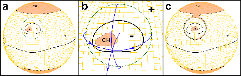
Figure 6: (a) Hypothetical topology satisfying uniqueness but still forbidden by the flux annulus argument. (b) Close-up of this topology inside the nested-polarity region. (c) Nested coronal hole topology that is not forbidden.

Open field corridors play a critical role in reconciling multipolar topologies with our uniqueness conjecture. Let us return to the topology of Fig. 4a, in which the active-region separatrix curve is well removed from the polar coronal-hole boundary, and consider the effect of opening a coronal hole inside the nested polarity, as sketched in Figs. 6a and 6b. This should be allowed by the uniqueness conjecture, because there would still be only one coronal hole per unipolar region on the Sun. But the annulus argument forbids the topology of Figs. 6a and 6b on two counts. First, consider any annulus of closed flux that surrounds the inner spine. The inner spine maps to the whole fan surface, which surrounds the nested polarity, therefore, any annulus surrounding the spine must map to an annulus surrounding the nested polarity. But in order to pass around the embedded polarity coronal hole, any such annulus of closed flux would have to split, which is not allowed. This problem is easily taken care by insisting that:
Any coronal hole that opens inside a nested polarity must encompass the spine.
This conclusion has important implications for models of CME initiation such as the breakout model (Antiochos, DeVore, & Klimchuk, 1999). It predicts that prior to eruption the inner spine should appear to move toward that part of the sheared PIL that eventually erupts. Furthermore, the amount of energy available for eruption will depend on how much the spine can move (Antiochos, DeVore, & Klimchuk, 1999; DeVore & Antiochos, 2005).

The second application of the annulus argument leads to a more surprising conclusion. Any annulus of closed flux that surrounds the polar coronal hole of Fig. 6a would clearly have to split even if the embedded coronal hole had a permissible, open-spine topology. It would appear, therefore, that the annulus argument implies not just one hole per unipolar region, but only one hole per polarity (i.e., only two on the whole Sun), which cannot be right. The resolution to this conundrum is illustrated by Fig. 6c – the formation of an open-field corridor that passes completely around the nested polarity region. In Fig. 6c, field line splitting is no longer a problem, because any annulus of closed flux that surrounds the main coronal hole must also surround the active-region hole. Also, any annulus of closed flux inside the nested region that surrounds the nested hole closes completely within the closed flux region of the nested polarity. These arguments imply that multiple coronal holes are, indeed, possible, but they must obey the following nesting conjecture:
Coronal holes of nested polarity regions must themselves be nested.

Although, the nesting conjecture imposes a powerful constraint on coronal hole topology, its importance for observed solar fields is uncertain. Nested coronal holes imply the presence of small conical current sheets in addition to the main heliospheric current sheet. In situ measurements usually indicate a single current sheet in the heliosphere, implying that there are only two coronal holes on the Sun. If so, then the issue of nested coronal holes becomes moot. Note that the nested polarity flux must be large in order to obtain a nested coronal hole within the context of the source surface model, in other words, a large active region far from the equator. This combination is rarely observed on the Sun, but still, it would be intriguing to search for any such nested holes in the published source surface maps, and then to search for their current sheets in the heliosphere.

Furthermore, the source surface model is likely to underestimate the occurrence of nested coronal holes, because this model does not include force balance between field and plasma. The topology of Fig. 5b contains a simple X-type null on the fan surface separating open and closed field. If plasma is added to the configuration of Fig. 5b, a difference in gas pressure will develop between the confined plasma inside the fan and the unconfined, solar wind plasma outside, just as there is a well-observed difference in the gas pressure between solar closed-field regions and coronal holes. For low beta, a gas pressure gradient across the fan or any other magnetic surface can readily be balanced by a small magnetic pressure gradient there; but, this is not possible near the null where the beta becomes infinite. It seems, therefore, that the plasma pressure would strongly deform the field near the null, and in some cases, may force open a finite region of flux around the inner spine even though the source surface model predicts no nested coronal hole. Of course, the nested polarity regions on the Sun are likely to be evolving via flux emergence or cancellation and photospheric motions. In fact, several models for accelerating the wind (Parker, 1992; Axford & McKenzie, 1992) and for forming polar plumes (DeForest & Gurman, 1998) invoke this process of interchange reconnection between the closed flux of an embedded bipole and surrounding open field. Therefore, it may be that any small nested holes are masked by the reconnection and dynamics. There are bound to be cases, however, where large quasi-static bipoles appear inside coronal holes. We predict that, at least for these cases, there would be a significant and possibly observable difference between the topology predicted by the source surface and the MHD model.

One situation in which the nesting conjecture is quite likely to play an important role is in long-lived dimming regions formed by CMEs. The dimming regions are believed to be transient coronal holes where the magnetic field has been forced open by a CME (Thompson et al., 2000). Since they are transient, it is not clear that our arguments above apply. If the holes are sufficiently long-lived (time scales of tens of hours), however, the quasi-steady assumption may still be valid. If so, then we can make two predictions on such “not-too-transient” holes. First, any dimming region that forms inside an active region PIL must encompass the inner spine. This prediction probably is difficult to test, because the inner spine is not easily observed (Aulanier et al., 2000). Second, the formation of such a dimming region must be accompanied by the formation of a transient coronal hole (possibly a very narrow open-field corridor) surrounding the PIL. This latter prediction may well be testable in some well-observed CMEs.

5 Discussion

Let us summarize our main findings and predictions on coronal hole topology. First, we list two supporting “lemmas”:
A coronal hole boundary cannot intersect a polarity inversion line.
This statement is rigorously valid for the quasi-steady models, because the heliospheric current sheet cannot extend down to the photosphere. In the interchange models, however, open flux is presumably free to diffuse across PILs, which emphasizes the striking difference between the two models.

A nested polarity region must be surrounded by either all open or all closed field.
The prediction from this result is that coronal hole boundaries undergo discontinuous jumps in response to bipolar regions entering or exiting the holes.

Next, application of the annulus-of-closed-flux argument leads to our two main results, the uniqueness and nesting conjectures:
Every unipolar region on the photosphere can contain at most one coronal hole.
We predict that seemingly disconnected holes are actually connected by observationally unresolved open field corridors. These corridors are likely to be dynamic, with the field continuously opening and closing in response to photospheric motions and flux emergence or submergence. Furthermore, we expect such corridors to be ubiquitous at the boundaries of coronal holes, causing these boundaries to have a fractal-like and inherently dynamic structure (see Fig. 2b). Consequently, the corridors may be an important source of the slow wind.

Coronal holes of nested polarity regions must themselves be nested.
The prediction is that if a coronal hole develops in an active region (i.e., a nested polarity region), then the polar coronal hole will grow to surround the nested polarity. This may hold even for transient coronal holes associated with CMEs. Related to this conjecture is the corollary:
Any coronal hole that opens inside a nested polarity must encompass the spine.

We emphasize that the statements are still conjectures, even for the quasi-steady models. The arguments presented in this paper used only basic topologies for the coronal field. It may well be that one can find counter-examples, especially in systems with special symmetries so that structures such as null lines or null surfaces appear in the corona. On the other hand, the coronal magnetic field is generally observed to have smooth structure without evidence for such topological pathologies. Note also that topologies such as null lines are structurally unstable, in general, so they would exist only as transient structures. Therefore, if our conjectures are valid for the topologies discussed above, it seems likely that they will hold for most observed solar magnetic fields.

We further emphasize that, for application to the Sun, all our results depend on the underlying assumption that the large-scale corona can be considered to be in a quasi-steady equilibrium state, as in the source surface and MHD models. If time-dependent effects dominate instead, as in the interchange models, then the statements above are unlikely to be valid. Consequently, observational testing of our conjectures may be the most effective method for determining the correct theory for the solar-heliospheric magnetic field.

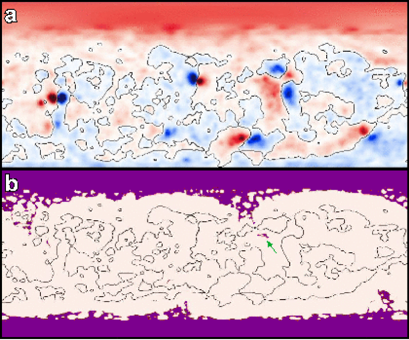
Figure 2: (a) Photospheric polarity from MDI magnetograms for Carrington rotation 1922. (b) Source surface solution showing open (purple) and closed (off white) regions along with the photospheric PIL (black lines). The apparently disconnected hole is marked by an arrow.

References

- Altschuler & Newkirk (1969) Altschuler, M. D. & Newkirk, G. 1969, Sol. Phys., 131
- Antiochos (1987) Antiochos, S. K. 1987, ApJ, 312, 886
- Antiochos (1990) Antiochos, S. K. 1990, J. Italian Astron. Soc., 61, 369
- Antiochos (1998) Antiochos, S. K. 1998, ApJ, 502, L181
- Antiochos, DeVore, & Klimchuk (1999) Antiochos, S. K., DeVore, C. R., & Klimchuk, J. A. 1999, ApJ, 510, 485
- Antiochos (2006) Antiochos, S. K. 2006, Eos Trans. AGU, 87(52), Fall Meet. Suppl., Abstract SH21B-04
- Arge & Pizzo (2000) Arge, C. N. & Pizzo, V. 2000, J. Geophys. Res., 105, 10465
- Arge et al. (2004) Arge, C. N., Luhmann, J. G., Odstrcil, D., Schrijver, C. J., & Li, Y. 2004, J. Atmos. Solar-Terrestrial Phys., 66, 1295
- Aulanier et al. (2000) Aulanier, G. DeLuca, E. E., Antiochos, S. K., McMullen, R. A., & Golub L. 2000, ApJ, 540, 1126
- Axford & McKenzie (1992) Axford, W. I. & McKenzie, J. F. 1992, in Solar Wind Seven, eds. E. Marsch & R. Schwenn (New York: Pergamon), 1
- Axford & McKenzie (1997) Axford, W. I. & McKenzie, J. F. 1997, in Cosmic Winds and the Heliosphere, eds. J. R. Jokipii, C. P. Sonnett, & M. S. Giampapa, (Tucson: Univ. of Ariz. Press), 31
- Cowley (1973) Cowley, S. W. H. 1973, Radio Science, 8, 903
- Crooker, Larson, & Kahler (2002) Crooker, N. U., Larson, D. E., & Kahler, S. W. 2002, J. Geophys. Res., 107:10.1029/2001JA000236
- DeForest & Gurman (1998) DeForest, C. E. & Gurman, J. B 1998, ApJ, 501, L217
- DeVore & Antiochos (2005) DeVore, C. R. & Antiochos, S. K. 2005, ApJ, 628, 1031
- Fan (2001) Fan, Y. 2001, ApJ, 554, L111
- Fisk, Zurbuchen, & Schwadron (1999) Fisk, L. A., Zurbuchen, T. H. & Schwadron, N. A. 1999, ApJ, 521, 868
- Fisk (2005) Fisk, L. A. 2005, ApJ, 626, 563
- Fisk & Zurbuchen (2006) Fisk, L. A. & Zurbuchen, T. H. 2006, J. Geophys. Res., 111:10.1029/2005JA011575
- Fletcher et al. (2001) Fletcher, L., Metcalf, T. R., Alexander, D., Brown, D. S., & Ryder, L. A. 2001, ApJ, 554, 451
- Forbes (2000) Forbes, T. G. 2000, J. Geophys. Res., 105, 23153
- Gosling (1990) Gosling, J. T. 1990, in Physics of Magnetic Flux Ropes, ed. C. T. Russell., E. R. Priest, & L. C. Lee, (AGU Geophys. Monograph 58), 373
- Greene (1988) Greene, J. M. 1988, J. Geophys. Res., 93, 8583
- Hoeksema (1991) Hoeksema, J. T. 1991, Adv. Space Res., 11, 15
- Howard et al. (1985) Howard, R. A., Sheeley, N. R., Jr., Michels, D. J., & Koomen, M. J. 1985, J. Geophys. Res., 90, 8173
- Hundhausen et al. (1984) Hundhausen, A. J., Sawyer, C. B., House, L., Illing, R. M. E., & Wagner, W. J. 1984, J. Geophys. Res., 89, 2639
- Jackson (1962) Jackson, J. D. 1962, Classical Electrodynamics, Ch. 2, (New York: Wiley & Sons)
- Kahler & Hudson (2002) Kahler, S. W. & Hudson, H. S. 2002, ApJ, 574, 467
- Karpen, Antiochos, & DeVore (1990) Karpen, J. T., Antiochos, S. K., & DeVore, C. R. 1990, ApJ, 356, L67
- Klimchuk (2001) Klimchuk, J. A. 2001, in Space Weather (AGU Monograph Series), eds P. Song, G. Siscoe, & H. Singer (Washington: AGU), 143
- Lau & Finn (1990) Lau, Y.-T. & Finn, J. M. 1990, ApJ, 350, 672
- Lin & Kahler (1992) Lin, R. P. & Kahler, S. W. 1992, J. Geophys. Res., 97, 8203
- Lin, Soon, & Baliunas (2003) Lin, J., Soon, W., & Baliunas, S. 2003, New Astronomy Reviews, 47, 53
- Linker et al. (1999) Linker, J. A. et al. 1999, J. Geophys. Res., 104, 9809
- Linker et al. (2003) Linker, J., Mikic, Z., Riley, P., Lionello, R., & Odstrcil, D. 2003, in SOLAR WIND TEN: Proceedings of the Tenth International Solar Wind Conference, AIP Conference Proceedings Vol. 679, 703
- Lionello et al. (2006) Lionello, R., Linker, J. A., Mikic, Z., & Riley, P. 2006, ApJ, 642, L69
- Low (2001) Low, B. C. 2001, J. Geophys. Res., 106, 25141
- Luhmann et al. (2002) Luhmann, J.G., Li, Y., Arge, C.N., Gazis, P. R., & Ulrich, R. 2002, J. Geophys. Res., 107, 1154
- Luhmann et al. (2003) Luhmann, J. G., Li, Y., Zhao, X., & Yashiro, S. 2003, Sol. Phys., 213, 367
- McComas et al. (1989) McComas, D. J., Gosling, J. L., Phillips, J. L., Bame, S. J., Luhmann, J., G., & Smith, E. J. 1989, J. Geophys. Res., 94, 6907
- McComas et al. (1991) McComas, D. J., Phillips, J. L., Hundhausen, A. J., & Burkepile, J. T. 1991, Geophys. Res. Lett., 18, 73
- Muller (1994) Muller, R. 1994, in Solar Surface Magnetism, ed. R. J. Rutten & C. J. Schrijver (Dordrecht: Kluwer), 55
- Odstrcil (2003) Odstrcil, D. 2003, Adv. Space. Res. 32, 497
- Pagel, Crooker, & Larson (2005) Pagel, C., Crooker, C. U., & Larson, D. E. 2005, Geophys. Res. Lett., 32:10.1029/2005GL023043
- Parker (1958) Parker, E. N. 1958, ApJ, 128, 664
- Parker (1983) Parker, E. N. 1983, ApJ, 264, 642
- Parker (1992) Parker, E. N. 1992, J. Geophys. Res., 97, 4311
- Parnell & Galsgaard (2004) Parnell, C. E. & Galsgaard, K 2004, A&A, 428, 595
- Pontin & Galsgaard (2004) Pontin, D. I. & Galsgaard, K 2007, J. Geophys. Res., 112:10.1029/2006JA011848
- Priest & Titov (1996) Priest, E. R., & Titov, V. S. 1996, Phil. Trans. R. Soc., 354, 2951
- Riley, Linker, & Mikic (2001) Riley, P., Linker, J., & Mikic, Z. 2001, J. Geophys. Res., 106, 15889
- Riley et al. (2003) Riley, P., Mikic, Z., Linker, J., & Zurbuchen, T. 2003, SOLAR WIND TEN: Proceedings of the Tenth International Solar Wind Conference, AIP Conference Proceedings 679, 79
- Roussev et al. (2003) Roussev, I. I., Gombosi, T. I., Sokolov, I. V., Velli, M., Manchester, W. IV, DeZeeuw, D., Liewer, P., Toth, G., & Luhmann, J. 2003, ApJ, 595, L57
- Schatten, Wilcox, & Ness (1969) Schatten, K., Wilcox, J. W., & Ness, N. F. 1969, Sol. Phys., 9, 442
- Schrijver et al. (1997) Schrijver, C. J. et al. 1997, Nature, 48, 424
- Schrijver & DeRosa (2003) Schrijver, C. J. & DeRosa, M. L. 2003, Sol. Phys., 212, 165
- Sheeley et al. (1975) Sheeley, N. R., Jr., Bohlin, J. D., Brueckner, G. E., Purcell, J. D., Scherrer, V., & Tousey, R. 1975, Sol. Phys., 40, 103
- Sheeley & Wang (2002) Sheeley, N. R., Jr. & Wang, Y.-M. 2002, ApJ, 579, 874
- Shibata et al. (1994) Shibata et al. 1994, ApJ, 431, L51
- Solanki (1993) Solanki, S. K. 1993, Space Sci. Rev. 63, 1
- Stern (1973) Stern, D. P. 1973, J. Geophys. Res., 78, 7292
- Syrovatskii (1981) Syrovatskii, S. I. 1981, ARA&A, 19, 163
- Thompson et al. (2000) Thompson, B. J., Cliver, E. W., Nitta, N., Delannee, C., & Delaboudiniere, J.-P. 2000, Geophys. Res. Lett., 27, 1431
- Timothy et al (1975) Timothy, A. F., Krieger, A. S. & Vaiana, G. S. 1975, Sol. Phys., 42, 135
- Titov, Priest, & Demoulin (1993) Titov, V. S., Priest, E. R., & Demoulin, P 1993, A&A, 276, 564
- Titov, Hornig, & Demoulin (2002) Titov, V. S., Hornig G., & Demoulin, P. 2002, J. Geophys. Res., 107:10.1029/2001JA000278
- Tousey et al. (1973) Tosey, R. et al. 1973, Sol. Phys., 33, 265
- Ugarte-Urra, Warren, & Winebarger (2007) Ugarte-Urra, I., Warren, H. P., & Winebarger A. R. 2007, ApJ, submitted
- van Ballegooijen (1985) van Ballegooijen, A. A 1985, ApJ, 298, 421
- Vourlidas et al. (1996) Vourlidas, A., Bastian, T. S., Nitta, N., & Aschwanden, M. J. 1996, Sol. Phys., 163, 99
- Wang & Sheeley (1990) Wang, Y-M. & Sheeley, N. R. Jr. 1990, ApJ, 365, 372
- Wang & Sheeley (1992) Wang, Y-M. & Sheeley, N. R. Jr. 1992, ApJ, 392, 310
- Wang, Hawley, & Sheeley (1996) Wang, Y.-M., Hawley, S. H., & Sheeley, N. R. Jr. 1996, Science, 271, 464
- Wu, Andrews, & Plunkett (2001) Wu, S.-T., Andrews, M., & Plunkett, S. 2001, Space Sci. Rev., 95, 191
- Zirker (1977) Zirker, J. B., ed. 1977, Coronal Holes and High-Speed Wind Streams, (Boulder: Colorado Associated University Press)
- Zurbuchen (2007) Zurbuchen, T. H. 2007, ARA&A, 45, in press