Scale-free avalanches in the multifractal random walk.

Abstract

Avalanches, or Avalanche-like, events are often observed in the dynamical behaviour of many complex systems which span from solar flaring to the Earth’s crust dynamics and from traffic flows to financial markets. Self-organized criticality (SOC) is one of the most popular theories able to explain this intermittent charge/discharge behaviour. Despite a large amount of theoretical work, empirical tests for SOC are still in their infancy. In the present paper we address the common problem of revealing SOC from a simple time series without having much information about the underlying system. As a working example we use a modified version of the multifractal random walk originally proposed as a model for the stock market dynamics. The study reveals, despite the lack of the typical ingredients of SOC, an avalanche-like dynamics similar to that of many physical systems. While, on one hand, the results confirm the relevance of cascade models in representing turbulent-like phenomena, on the other, they also raise the question about the current state of reliability of SOC inference from time series analysis.

1 Introduction

The theory of self-organized criticality (SOC) has been developed in the late eighty’s by Bak, Tang and Wiesenfeld Bak8788 , in order to explain the ubiquity of power laws in nature. The key concept of SOC is that complex systems “naturally” self-organize to a globally stationary intermittent state in which avalanche-like events are power law distributed. These features are similar to those found in physical systems at the critical point Jensen . The prototypical model of a system exhibiting SOC behaviour is the 2D sandpile Bak8788 . Here the cells of a grid are filled by randomly dropping grains of sand (external driving). When the gradient between two adjacent cells exceeds a certain threshold a redistribution of the sand occurs, leading to more instabilities and further redistributions. The characteristics of this system, indeed of all systems exhibiting SOC, is that the distribution of the avalanche sizes, their duration and the energy released, obey power laws.

Remarkably, this kind of scale-free intermittent evolution is similar to that observed in many physical and social systems. Examples include astrophysical and geophysical plasmas flares ; spplasma , earthquakes earthquake , evolutions of species Bak93 , traffic dynamics traffic , wars Roberts98 and the stock market Turcotte99 ; Bak93b ; Bak97 ; Feigenbaum03 (a recent review on the subject can be found in Ref. Turcotte99 ). Despite the theoretical interest, reliable tests to prove the presence of SOC in real systems are still in their infancy. Some attempts have been made in the contest of solar flaring Boffetta99 , astrophysical Bruno01 ; Lepreti04 and laboratory Spada01 ; Antoni01 plasmas and the stock market Bartolozzi05 . These works, while leaving open the question of a SOC behaviour, clearly show that the evolution of these systems can be well described by an avalanche-like dynamics characterized by power laws in the avalanche size, duration and waiting time between them. The presence of correlation between laminar times, that is the time elapsed between two avalanches, in particular, has raised objections to the relevance of SOC in these contexts. In fact, due to the lack of memory in the random external driving commonly used in the simulations of conservative SOC systems, the probability distribution function (PDF) of laminar times actually follows an exponential decay Wheatland98 . However, for non-conservative systems, power laws can still be observed in the presence of temporal correlations of the avalanches near the SOC state Freeman00 ; Carvalho00 . Such temporal correlation could also be due to the intrinsic memory process (possibly chaotic) in the driver DeLosRios97 ; Sanchez02 .

Motivated by recent observations of avalanche-like dynamics in financial time series Bartolozzi05 , we investigate a possible similar behaviour in the popular multifractal random walk (MRW) originally proposed in Ref. Bacry01 as a paradigm for the stock market behaviour. This model, although not presenting the characteristic mechanisms of SOC, such as a threshold triggering for the avalanches, is able to reproduce most of the stylized features of the stock market. Moreover, the MRW belongs to a family of cascade-like models widely used to reproduce the statistical features of the velocity fluctuations in hydrodynamic turbulence and, therefore, the discussions outlined in the next sections go beyond their application to finance but can be extended to every complex system which displaying a turbulent-like dynamics.

In the next section we introduce the asymmetric MRW proposed by Chen, Jayaprakash and Yuan Chen05 , which avalanche dynamics is investigate in detail in the rest of the paper. In Sec. 3 we introduce the method of analysis while the results are exposed in Sec. 4. Discussions and conclusions are left for the last section.

2 The MRW Model: the CJY Version

Recently, the study of the stock market, seen as a complex system, has attracted the attention of many physicists (for reviews see Refs. Mantegna99 ; Bouchaud99 ; Paul99 ; Feigenbaum03 ). Its dynamical behaviour is characterized by “stylized facts” mainly concerning the logarithmic returns, $r(t)=\ln\left[P(t)/P(t-1)\right]$ (where $P(t)$ is the stock price), and their absolute values, that can be regarded as a measure of the volatility, $v(t)=|r(t)|$. Such stylized facts have been used as a guide for validating phenomenological models of stock price fluctuations. Among them, the appearance of “fat tails” in the PDF of the logarithmic returns, related to frequent large fluctuations in price, and the long time correlations present in the volatility, a phenomenon known as volatility clustering, have been extensively investigated in the econophysics literature Kaizoji00 ; Krawiecki02 ; Takayasu9798 ; Bartolozzi . The evidence of leptokurtic distributions in financial time series leads to immediate analogies with the longitudinal fluctuations of turbulent flows where a similar dynamics is observed, although differences have been pointed out as well Mantegna99 . Motivated by the aforementioned evidence, cascade models, originally developed to reproduce the characteristic features of intermittency in hydrodynamic turbulence, have been applied, with success, to reproduce some stylized facts of the stock market dynamics.

In this framework, one of the most popular models is the MRW originally proposed by Bacry, Delour and Muzy Bacry01 . The version that we are going to use in the present investigation has been proposed by Chen, Jayaprakash and Yuan Chen05 , referred to as CJY in the rest of the paper. In the CJY model the returns are expressed by

$$r(t)=\delta_{t}\,z_{t},$$ (1)

where $z_{t}$ is a Gaussian random variable with zero mean and unitary standard deviation, while $\delta_{t}$ represents the one-step volatility. The dynamics of the model, and therefore the capability to reproduce the stylized facts of the stock market, is related to the dynamics of the variable $\delta_{t}$: small variations lead to an intermittent behaviour in $r(t)$, similar to the one observed in the financial markets. Specifically, we can write $\delta_{t}$ as

$$\delta_{t}=\delta_{0}\,\gamma^{n(t)},$$ (2)

where $\delta_{0}$ is related to the amplitude of the fluctuations while $\gamma$ to their intermittency. The term $n(t)$, the core of the model, is a bounded random walk with increments

$$\Delta n(t)=\eta_{t}+\alpha\,\Psi(t)-\beta\,\bar{\eta}.$$ (3)

Here

$$\Psi(t)=K_{1}\,\eta_{t}-K_{N_{c}+1}\,\eta_{t-N_{c}-1}+\sum_{i=1}^{N_{c}}[K_{i+1}-K_{i}]\,\eta_{t-i},$$ (4)

with $\eta_{t}$ independent random variables, with average $\bar{\eta}$, which assume the values +1 with probability $p$ and $-1$ with probability $1-p$. In our simulations $\bar{\eta}=2p-1<0$. This term, that alone can reproduce volatility clustering, has been found to be necessary in order to reproduce some scaling properties of the conditional fluctuations observed in financial data Chen05 . The second term in the increment, $\Psi(t)$, has the ability to recover the long-time correlations of the market volatility and, from now on, we will refer to it as the multifractal increment. Its strength coefficient, $\alpha$, is related to the degree of intermittency of the time series and, therefore, to the time scale of process. The kernel used in Eq.(4) for the convolution is $K_{i}=1/\sqrt{i}$ and we fix the memory steps to $N_{c}=1000$ in the simulations. The last term of Eq. (3), controls the drift rate in $n(t)$, instead, with strength $\beta$, and, therefore, adds more flexibility to the model. A more detailed discussion on the present model with $\alpha=\beta=0$ can be found in Ref. Chen03 . The parameter $\gamma$ is fixed to $1.05$ in all the simulations and, following Ref. Chen05 , it is linked to $\alpha$ and $p$ according to:

$$\alpha=\frac{\alpha_{0}}{\ln(\gamma)},$$ (5)

$$p=\frac{1}{1+\gamma^{2}}.$$ (6)

These particular choices are appropriate for a correct reproduction of the observed statistical features of the data. Note also that, for the previous choice of the parameter $\gamma$, namely 1.05, the probability distribution of the random variable in the multifractal increment, Eq.(6), becomes slightly asymmetric, $p=0.4756$, in contrast with the symmetry of the original MRW Bacry01 . As previously mentioned, we impose reflecting boundaries for $n(t)$ in order to prevent the realization of extremely large or small (unrealistic) fluctuations in the simulation of the market activity, namely $0\leq n(t)\leq n_{max}$, with $n_{max}=\ln(30)/\ln(\gamma)$. By doing that, $\delta_{t}$ in Eq.(1) is bounded between $\delta_{0}$ and $30\,\delta_{0}$.

In Fig. 1 we compare the time series generated with the model of Eqs. (2) and (3), Fig. 1 (b), and the time series of daily returns for the S&P500 index, Fig. 1 (a). The parameters used in the simulation, and reported in the caption of the figure, have been chosen in order to match the properties of the financial data set, as underlined by the similarities in the PDFs of the two processes, Fig. 1 (c). Note, however, some discrepancies in the tails of the PDFs. A possible explanation is that the dynamics of the extreme events differs from the dynamics of the bulk of the distribution (generated by the CYJ model, in this case) and they could be interpreted as “outliers” Johansen98 ; Sornette_book . However, finite size effect in the relatively short time series of the S&P500 should be also considered.

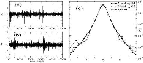
Figure 1: (a) Part of the time series of logarithmic returns for daily data of the S&P500 index, used to calculate the PDF in (c). The all set spans from 3/1/1950 to 18/7/2003. (b) Time series generated from the model of Eqs. (2) and (3) with parameters $\gamma=1.05$, $\alpha_{0}=0.1$, $\beta=1.3$ and $\delta_{0}=1$. The two time series shown in the plot have been standardized according to $r(t)\rightarrow(r(t)-\langle r\rangle)/\sigma(r)$, where $\langle\ldots\rangle$ and $\sigma$ represent, respectively, the average and the standard deviation over the period in examination. (c) Comparison between the PDFs in (a) and (b). The PDF generated with the parameters $\gamma=1.05$, $\alpha_{0}=0.2$, $\beta=4.0$ and $\delta_{0}=1$ is also shown.

3 Wavelet Transform Filtering and Analysis Method

As mentioned in the introduction, many complex systems show an intermittent activity: quiescent periods are suddenly interrupted by bursts of activity. This kind of non-stationary dynamics is often related to multi-scale phenomena and most of the time standard analysis techniques can fail to reveal some important events that are localized in time or scale Frisch . This is, for example, when using elementary filters: along with the noise background also meaningful information can be filtered out Bartolozzi05 .

In order to overcome these problems, wavelet based techniques are becoming more and more popular in complex systems applications Farge92 . This approach enables one to decompose the signal in terms of scale and time units and so to separate its coherent parts (or “avalanches”) – that is, the bursty periods related to the tails of the PDF – from the noise-like background, thus enabling an independent study of the intermittent and the quiescent intervals Farge99 ; Spada01 ; Bruno01 ; Kovacs01 ; Bartolozzi05 .

The idea behind the wavelet transform is similar to that of windowed Fourier analysis and it can be shown that the scale parameter is indeed inversely proportional to the classic Fourier frequency. The main difference between the two techniques lies in the resolution in the time-frequency domain. In Fourier analysis the resolution is scale independent, leading to aliasing of high and low frequency components that do not fall into the frequency range of the window. However, in the wavelet decomposition the resolution changes according to the scale (i.e. frequency). At smaller scales the temporal resolution increases at the expense of frequency localization, while for large scales we have the opposite. For this reason the wavelet transform can be considered a sort of mathematical “microscope”. While the Fourier analysis is still an appropriate method for the study of harmonic signals, where the information is equally distributed, the wavelet approach becomes fundamental when the signal is intermittent and the information localized.

For a time series analysis it is often preferable to use a discrete wavelet transform (DWT). The DWT can be seen as a appropriate sub-sampling of the continuous wavelet transform (CWT) by using dyadic scales. That is, one chooses $\lambda=2^{j}$, for $j=0,...,L-1$, where $L$ is the number of scales involved, and the temporal coefficients are separated by multiples of $\lambda$ for each dyadic scale, $t=n2^{j}$, with $n$ being the index of the coefficient at the $j$th scale. The DWT coefficients, $W_{j,n}$, can then be expressed as

$$W_{j,n}=\langle f,\psi_{j,n}\rangle=2^{-j/2}\int f(u)\psi(2^{-j}u-n)du,$$ (7)

where $\psi_{j,n}$ is the discretely scaled and shifted version of the mother wavelet. The wavelet coefficients are a measure of the correlation between the original signal, $f(t)$, and the mother wavelet, $\psi(t)$ at scale $j$ and time $n$. For the DWT, if the set of the mother wavelet and its translated and scaled copies form a complete orthonormal basis for all functions having a finite squared modulus, then the energy of the starting signal is conserved in the wavelet coefficients. This property is, of course, extremely important when analyzing physical time series Kovacs01 . Following Ref. Bartolozzi05 , we use the Daubechies-4 as mother wavelet Daubechies88 for the analysis presented in the next sections. Tests performed with different sets do not lead to any qualitative difference in the results. A more comprehensive discussions on the general properties of wavelets and their applications are given in Refs. Daubechies88 ; Farge92 .

The importance of the wavelet transform in the study of turbulent-like signals lies in the fact that the large amplitude wavelet coefficients are related to the extreme events in the tails of the PDF, while the laminar or quiescent periods are related to the ones with smaller amplitude Kovacs01 . In this way it is possible to define a criterion whereby one can filter the time series of the coefficients depending on the specific needs. In our case we adopt the method used in Refs. Kovacs01 ; Bruno01 ; Bartolozzi05 and originally proposed by Katul et al. Katul94 . In this method wavelet coefficients that exceed a fixed threshold are set to zero, according to

$$\tilde{W}_{j,n}=\left\{\begin{array}[]{ccc}W_{j,n}&{\rm if}&W^{2}_{j,n}<C\cdot\langle W^{2}_{j,n}\rangle_{n},\\ 0&{\rm otherwise},\end{array}\right.$$ (8)

here $\langle\ldots\rangle_{n}$ denotes the average over the time parameters at a certain scale and $C$ is the threshold coefficient. Once we have filtered the wavelet coefficients $\tilde{W}_{j,n}$ we perform an inverse wavelet transform, obtaining a smoothed version of the original time series.

The residuals of the original time series with the filtered one correspond to the bursty periods, or avalanches, which we aim to study. An example of the filtering technique in terms of PDFs is given in Fig. 2.

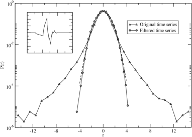
Figure 2: PDFs of the original time series, Fig. 3 (a), obtained with the model of Eq. (2) ($\gamma=1.05$, $\alpha_{0}=0.1$, $\beta=1.3$ and $\delta_{0}=1$) and its filtered version, Fig. 3 (b). A Gaussian is also plotted for visual comparison (dashed line). The Daubechies-4 wavelet used for the analysis is shown in the inset.

Once we have isolated the noise part from our signal series we are able to perform a reliable statistical analysis on the avalanches of the residual time series. In particular, we define the avalanches as the set of events during which the volatility of the residual time series, $v_{res}(t)\equiv|r_{res}(t)|$, is constantly above a positive small threshold, $\epsilon\approx 0$. It is also possible to find an optimal value for the choice of the threshold parameter $C$ in a way that the filtered time series is, as close as possible, uncorrelated Gaussian noise. From previous studies, this parameter is found to be $C\sim 1$ Bartolozzi05 . In any case, the resulting statistical analysis is qualitatively unchanged as long as $0\lesssim C\lesssim 4$ Kovacs01 ; Bartolozzi05 . A graphic example of the procedure for extracting the avalanches is illustrated in Fig. 3.

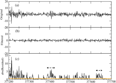
Figure 3: (a) Window of the time series obtained with the model of Eq. (2) ($\gamma=1.05$, $\alpha_{0}=0.1$, $\beta=1.3$ and $\delta_{0}=1$). (b) Filtered version of the time series in (a) obtained with the Daubechies-4 wavelet. In order to properly identify the avalanches we create a residual time series by subtracting the filtered time series from the original one. This noise removal technique presents advantages to standard threshold methods when applied to multiscale systems Bartolozzi05 . (c) Absolute value of the residuals, or residual volatility, used to extract the avalanches, as explained in the text. Two examples of avalanches, among the many preset, are underlined by the dashed lines in (c). The horizontal line slightly above zero represents the small threshold $\epsilon$.

In analogy with the dissipated energy in a turbulent flow, we define the size of an avalanche, $E$, as the integrated value of the squared volatility over each coherent event of the residual time series. The duration, $D$, is defined as the interval of time between the beginning and the end of a coherent event, while the laminar time, $L$, is the time elapsing between the end of an event and the beginning of the next one.

4 Time Series Analysis

In the previous section we have seen how the wavelet multi-scale filtering technique is an excellent tool to remove uncorrelated Gaussian noise from an input signal. In particular, this filtering method becomes relevant whenever the examined time series presents an intermittent behaviour, that is an irregular switching, between periods characterized by large fluctuations and noise-like ones. By using this technique, the avalanches, which characterize an emergent behaviour in the dynamics, are highlighted at the expense of the uninteresting background. In this way we can make a proper statistical analysis of the quantities that characterize these coherent events, Fig. 3.

The statistical study of the avalanches identified with the wavelet technique is of great interest, not only because this would further test the capability of this model to reproduce the stylized facts of the stock market, but it could also shed some light on the relevance of this test in distinguishing between SOC and non-SOC processes in a time series analysis.

The analysis is carried out by studying how the statistics of the avalanches change as we tune the parameters of the CJY model. The time series generated with this algorithm have a length $N\sim 5\cdot 10^{5}$ ($N=2^{19}$). Moreover, we investigate the specific relevance of each term composing the increments of the variable $n(t)$, Eq.(3). In order to do this, we independently analyze the time series generated with different expressions for the increments, $\Delta n(t)$: for each simulation we consider a random walk for $n(t)$ with boundaries $n_{min}=0$ and $n_{max}=\ln(30)/\ln(\gamma)$.

We also fix $C=1$ as the threshold coefficient for the wavelet analysis. This particular value of $C$ is close to the optimization value in the de-noise procedure. However a different choice of this parameter would not change the qualitative results of our analysis Bartolozzi05 .

4.1 The Role of Multifractal Increments

We first investigate the avalanche dynamics generated by the multifractal increments, that is the part of the CJY model that is related to the original formulation of the MRW. In this case Eq.(3) reads as

$$\Delta n(t)=\alpha\,\Psi(t),$$ (9)

where $\Psi(t)$ is given by Eq.(4) and the strength coefficient is expressed by $\alpha=\alpha_{0}/\ln(\gamma)$ with $\gamma=1.05$.

The avalanche analysis, resulting from the wavelet filtering, for the size $E$, duration $D$, and laminar times $L$, is carried out for different values of $\alpha_{0}$. This parameter, and $\alpha$ as a consequence, is related to the degree of intermittency of the time series and, therefore, to the time scale of the process. For $\alpha_{0}\lesssim 0.05$, the dynamics of $r(t)$ is dominated by noise and its PDF is a Gaussian. In the stock market contest, as well as in turbulence, this corresponds to observe the fluctuations at large scales. As we move this parameter toward larger values, the time series of $r(t)$ becomes more and more intermittent, giving rise to the large fluctuations which characterize the broad tails of the PDFs of turbulent phenomena at small scales. The results are shown in Figs. 4, 5 and  6.

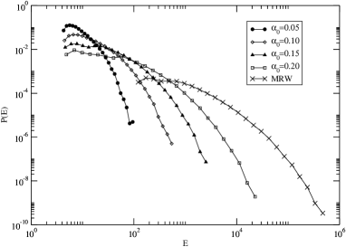
Figure 4: PDFs of the avalanche sizes, $E$, as a function of the parameter $\alpha_{0}$. For each value of this parameter the time series of $E$ is noise-like and the correspondent distribution displays an exponential decay. The strength $\alpha_{0}$ controls the decay rate of the distribution. The PDF for the MRW (X) with $\alpha=0.25$ is reported as well.

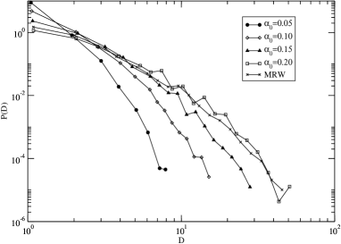
Figure 5: PDFs of the duration, $D$, for the purely multifractal model. No power law behaviour is observed and the same considerations as for the size, $E$, hold in this case. The PDF for the MRW (X) with $\alpha=0.25$ displays a similar behaviour.

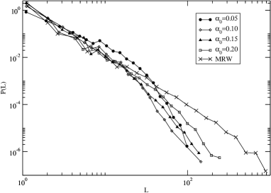
Figure 6: Distribution of laminar times, $L$, in the multifractal model. A slow convergence from an exponential decay to a power law one is observed for $\alpha_{0}\gtrsim 0.2$. The exponent of the power law, in this case, is $\nu\sim 2.3$. In this case the PDF for the MRW (X), with $\alpha=0.25$, displays a clearer power law behaviour compared to the CYJ version.

From these plots it is possible to observe how the purely multifractal model is not able to reproduce the power law behaviour observed in real data sets. In particular, the PDFs for $E$ and $D$ of the avalanches decay exponentially, independently on the value of $\alpha_{0}$. This is an indication of the randomness behind the avalanche generation process. The distribution of laminar times in Fig. 6, instead, show a Poisson-like shape for small values of this parameter, $\alpha_{0}=0.05$, while they start slowly to converge toward a power law shape, $P(L)\sim L^{-\nu}$, for $\alpha_{0}\gtrsim 0.2$. The resulting exponent, $\nu\sim 2.3$, is similar to the one found in the empirical studies Bartolozzi05 .

For completeness, we study also the avalanche dynamics by using the standard implementation of the MRW Sornette03 . In this case $\delta_{t}=\delta_{0}e^{n(t)}$ and $\Delta n(t)$ is given by Eq. (9) where, this time, $\eta_{t}$ is a Gaussian random variable with zero mean and unitary standard deviation. The shapes of the PDFs of $E$ and $D$ resulting from the analysis, shown in the Figs. 4 and  5 for $\alpha=0.25$, display a similar $\alpha$ dependence as the CYJ version, as expected. However, the PDF of laminar times, at least at small temporal scales, Fig.6, display a clearer power low behaviour compared to the CYJ model.

4.2 The Complete CJY Model

We turn now our attention to the complete CYJ model of Eq.(3). In this case, it has been shown Chen05 that a proper tuning of the parameters can reproduce most of the stylized features of the stock market. A particular good agreement between the model and the empirical data has been found by fixing $\gamma=1.05$ and $\delta_{0}=1.0$, for the two couples of parameters $(\alpha_{0}=0.1,\beta=1.3)$ and $(\alpha_{0}=0.2,\beta=4.0)$ as strength parameters for the memory term and the drift respectively. It is, therefore, of particular interest to explore the avalanche behaviour using these parameters. The results of the analysis are shown in Figs. 7, 8 and 9 for $E$, $D$ and $L$.

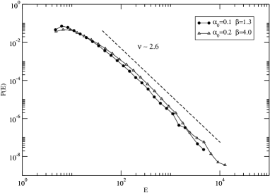
Figure 7: PDFs of the size, $E$, in the case $(\alpha_{0}=0.1,\beta=1.3)$ and $(\alpha_{0}=0.2,\beta=4.0)$. A similar power law shape, with exponent $\nu\sim 2.6$, is observed for the two distributions. A dashed line is also plotted for visual comparison.

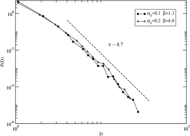
Figure 8: PDFs for the avalanches duration, $D$, for the same parameters of Fig. 7. In this case a power law with exponent $\nu\sim 4.7$, is observed.

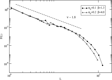
Figure 9: PDFs for the laminar times between avalanches, $L$. The parameters used are the same as in Fig. 7. A power law with exponent $\nu\sim 1.8$ and a cut-off at $L\sim 10^{2}$ is reported.

In this case, for some order of magnitude, we find a power law behaviour for the quantities under consideration. This is in qualitative agreement with the results found for the stock market. In particular, the exponents of the power laws seem to be close to the ones found for the analysis of the tick-by-tick Nasdaq E-mini Futures Bartolozzi05 . Note that a scale-free avalanche dynamics has also been observed in other reduced models of turbulence, the shell models Boffetta99 , via a simple threshold technique.

This result can have important consequences regarding the possible identification of SOC in the stock market, and other complex systems in general, through a time series analysis. In fact, we have shown that an avalanche-like behaviour can also be observed in models, such as the one presented in this work, in which the characteristic ingredients of SOC, such as threshold dynamics, are actually missing. This, of course, does not rule out the possibility of SOC but, nevertheless, more relevant and discriminating tests become necessary.

We further investigate our model by studying how the distribution of the $E$, $D$ and $L$ change with the drift strength $\beta$. In fact, different markets could have different power law exponents, no universality has been found until now, and we want to test the elasticity of the CYJ with respect to this parameter. The PDFs for $E$, $D$ and $L$ as functions of $\beta$ are reported, respectively, in Figs. 10, 11 and 12.

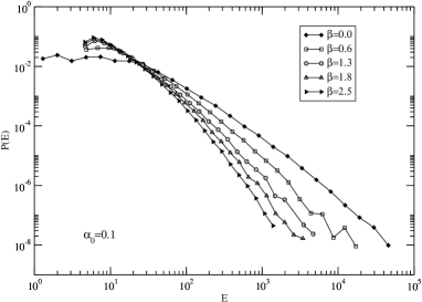
Figure 10: Dependence on the parameter $\beta$, with $\alpha_{0}=0.1$, for the PDF of the size, $E$, of the avalanche. The drift strength controls the slope of the power law, which appear to go to saturation for the higher values of $\beta$.

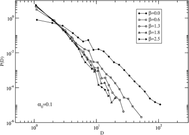
Figure 11: Dependence on the parameter $\beta$, with $\alpha_{0}=0.1$, for the PDF for the duration $D$ of the avalanches. Also in this case, the drift strength controls the slope of the PDF and saturates for large $\beta$.

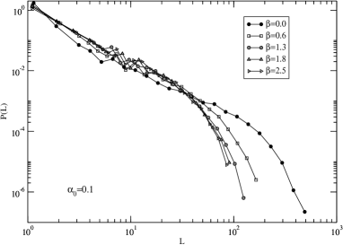
Figure 12: The exponent of the power law of the laminar times between the avalanches, $L$, do not seem to be sensitive to changes in the parameter $\beta$, which appear to be relevant just in changing the cut-off of the distribution.

The analysis shows how the parameter $\beta$ plays an important role in the dynamics of the model. In fact, although the shape of the PDFs for $E$ and $D$ are robust against variations of $\beta$, the exponent changes with this parameter. Higher values of $\beta$ imply a larger value for $\nu$. The same arguments do not hold for the statistics of the laminar times, $L$. In this case the resulting distribution is pretty much independent of $\beta$ and could constitute a limit in the present formulation of the model. A separate discussion is reserved for $\beta=0$. In this case the filtering procedure, with $C=1$ as optimal value, is not able to remove all the wavelet coefficients related to the large fluctuations. As a consequence, the excess of kurtosis, $K_{e}=\langle r^{4}\rangle/\langle r^{2}\rangle^{2}-3$, of the filtered time series, although still small in absolute value, $K_{e}\sim 0.2$, becomes more than one order of magnitude larger that in the previous analysis . This means, to some extent, that there is not enough Gaussian noise to be filtered out in the time series! Moreover, the shapes of the PDFs related to the avalanche dynamics, show a behaviour that is systematically different from the one observed once the drift is included, Figs. 10, 8 and 12.

As a final note, we consider, for $\beta=1.3$ fixed, how our analysis would change in the absence of the multifractal increment, $\alpha\,\Psi(t)$, in Eq.(3). In doing so, we compare the case with $\alpha_{0}=0.1$ and $\alpha_{0}=0$. The results are shown in Fig. 13.

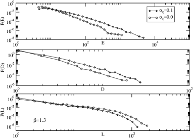
Figure 13: PDFs for $E$ (Top), $D$ (Middle) and $L$ (Bottom) for $\beta=1.3$ and $\alpha_{0}=0.1$, with multifractality, and with $\alpha_{0}=0$, without the multifractal term.

While the lack of the multifractal/memory term does not alter the distribution of laminar times between the clusters of volatility, it does increase the steepness of the distribution of $E$ and $L$. This result is actually expected since this term builds the correlations inside periods of high volatility of the market time series, that is the so-called volatility clustering. By removing it we explicitly cut off part of the correlations inside the model, resulting in shorter avalanches.

5 Discussion and conclusion

In the present work we investigated a possible avalanche-like dynamics in an extended version of the popular multifractal random walk, the CJY, proposed as a paradigm for the stock market dynamics. We have been able to identify avalanche-like events in the fluctuations generated by this model. Subsequently, the statistical properties of these events have been estimated. The identification of these clusters goes through an intermediate passage where we use a wavelet filtering technique in order to suppress the contribution of the noise background and, therefore, enhance the precision of our measures.

The results show that, for a broad range of the parameters, the distribution of size, duration and laminar time between avalanches follow a power law distribution. A very similar behaviour has been found in empirical studies on financial time series Bartolozzi05 . Therefore, we confirm the relevance of the cascade models, and in particular the CYJ version of the MRW, in modelling financial market. Our results also extend beyond the financial environment since this framework is quite general for describing dissipative, intermittent, systems, such as solar flaring or MHD turbulence, where an avalanche-like dynamics has been observed as well Boffetta99 ; Bruno01 ; Lepreti04 ; Spada01 ; Antoni01 .

Equally important, our results stress how models lacking of typical SOC mechanisms can, nevertheless, manifest an avalanche-like behaviour. In fact, the recognition of SOC “patterns” could be an artifact of the identification method itself. In this regard, it is worth mentioning that simple threshold techniques, when applied to time series generated by SOC-free processes, can lead to the identification of avalanches with size distributions (according to some specific definition) that are power laws. For example, it is well known that the “time for first return to the origin” of a random walk is power law distributed Sornette_book despite the lack of any correlation in the time series. A more sophisticated example is reported in Ref. Carbone04 where it has been shown that the behaviour of a self-affine fractional Brownian motion, when analyzed with a moving average technique, can mimic the avalanche dynamics of the Dhar-Ramaswamy sandpile. These results illustrate the technical ambiguity in the identification of SOC from time series. As long as we do not have any a priori information about the underlying dynamics of the system, it is very hard to tell if the avalanches that we observe are a result of a genuine SOC dynamics or any other diffusive process.

In conclusion, SOC has been claimed, perhaps too loosely, to play a role in many complex systems, but there is no method that is reliable enough to test its presence from the analysis of noisy time series. This is a very relevant issue since, in practical situations, all the available information regarding a system is encoded in its time series. Therefore, an extension of this theoretical framework, which would enable the present gap with empirical analysis to be filled, is of great practical importance and would probably settle many speculations on the subject.

References

- (1) P. Bak C. Tang and K. Wiesenfeld, Phys. Rev. Lett. 59, 381 (1987); P. Bak, C. Tang and K. Wiesenfeld, Phys. Rev. A 38, 364 (1988).
- (2) H. J. Jensen, Self-Organized Criticality: Emergent Complex Behavior in Physical and Biological Systems, (Cambridge University Press, Cambridge, 1998).
- (3) E.T. Lu and R.J. Hamilton, Astrophys.J. 380, L89 (1991); E.T. Lu et al., Astrophys.J. 412, 841 (1993).
- (4) T. Chang et al., Advances in Space Environmental Research, Vol.I, (Kluwer Academic Publisher,AH Dordrecht, The Netherlands, 2003); A. Valdiva et al., Advences in Space Environmental Research, Vol.I, (Kluwer Academic Publisher,AH Dordrecht, The Netherlands, 2003).
- (5) P. Bak and C. Tang, J. Geophys. Res. 94, 15 635 (1989); Sornette A. and Sornette D., Europhys. Lett. 9, 197 (1989); D. Sornette, P. Davy and A. Sornette, J. Geophys. Res. 95, 17 353 (1990); J. Huang et al., Europhys. Lett. 41, 43 (1998).
- (6) P. Bak and K. Snappen, Phys. Rev. Lett. 71, 4083 (1993).
- (7) K. Nagel and H.J. Herrmann, Physica A 199, 254 (1993); K. Nagel and M. Paczuski, Phys. Rev. E 51, 2909 (1995); T. Nagatani, J.Phys. A:Math.Gen. 28, L119 (1995); T. Nagatani, Fractals 4, 279 (1996).
- (8) D.C. Roberts and D.L. Turcotte, Fractals 6, 351 (1998).
- (9) D. L. Turcotte, Rep. Prog. Phys. 62, 1377 (1999).
- (10) P. Bak, K. Chen, J.Scheinkman and M. Woodford, Ric. Econ. 47, 3 (1993).
- (11) P. Bak, M. Paczuski and M. Shubik, Physica A 246, 430 (1997).
- (12) J. Feigenbaum, Rep. Prog. Phys. 66, 1611 (2003).
- (13) G. Boffetta et al., Phys. Rev. Lett. 83, 4662 (1999).
- (14) R. Bruno et. al., Planet. Space Sci.49, 045001 (2001).
- (15) F. Lepreti et. al., Planet. Space Sci.52, 957 (2004).
- (16) E. Spada et. al., Phys. Rev. Lett. 86, 3032 (2001).
- (17) V. Antoni et. al., Phys. Rev. Lett. 87, 045001 (2001).
- (18) M. Bartolozzi, D.B. Leinweber and A.W. Thomas, Physica A 350, 451 (2005); M. Bartolozzi, D.B. Leinweber and A.W. Thomas, Physica A 370, 132 (2006).
- (19) M.S. Wheatland, P.A. Sturrock, J.M. McTiernan, Astrophys.J.509, 448 (1998).
- (20) M.P. Freeman, N.W. Watkins and D.J. Riley, Phys. Rev. E 62, 8794 (2000).
- (21) J.X. Carvalho and C.P.C. Prado, Phys. Rev. Lett., 84, 4006 (2000).
- (22) P. De Los Rios, A. Valleriani and J.L. Vega, Phys. Rev. E 56, 4876 (1997).
- (23) R. Sanchez, D.E. Newman and B.A., Phys. Rev. Lett. 88, 068302-1 (2002).
- (24) E. Bacry, J. Delour and J.F. Muzy, Phys. Rev. E, 64, 026103 (2001); E. Bacry, J. Delour and J.F. Muzy, Physica A, 299, 84 (2001).
- (25) K. Chen, C. Jayaprakash and B. Yuan, arXiv: physics/0503157.
- (26) R. N. Mantegna and H. E. Stanley, An Introduction to Econophysics: Correlation and Complexity in Finance, (Cambridge University Press, Cambridge, 1999).
- (27) J.-P. Bouchaud and M. Potters, Theory of Financial Risk, (Cambridge University Press, Cambridge, 1999).
- (28) W. Paul and J. Baschnagel, Stochastic Processes: From Physics to Finance, (Spriger-Verlag, Berlin,1999).
- (29) T. Kaizoji, Physica A 287, 493 (2000).
- (30) A. Krawiecki, J.A. Holyst and D. and Helbing, Phys. Rev. Lett.89, 158701 (2002); A. Krawiecki and J.A. Holyst, Physica A 317, 597 (2003).
- (31) H. Takayasu, A.-H. Sato and M. Takayasu, Phys. Rev. Lett. 79, 966 (1997); H. Takayasu and M. Takayasu, Physica A 269, 24 (1999).
- (32) M. Bartolozzi and A.W. Thomas, Phys. Rev. E 69, 046112 (2004); M. Bartolozzi, D.B. Leinweber and A.W. Thomas, Phys. Rev. E 72, 046113 (2005).
- (33) U. Frisch, Turbulence, (Cambridge University Press, Cambridge, 1995).
- (34) S. Ghashghaie et al., Nature 381, 767 (1996).
- (35) A. Arneodo, J.F. Muzy and D. Sornette, Eur. Phys. J. B 2, 277 (1998).
- (36) W. Breymann, S. Ghashghaie and P. Talkner, International Journal of Theoretical and applied Finance 3, 357 (2000).
- (37) L. Calvet and A. Fisher, Journal of Econometrics 105, 27 (2001); L. Calvet and A. Fisher, Review of Economics and Statistics 84, 381 (2002).
- (38) T. Lux, Quant. Finance 1, 632 (2001); T. Lux, Int. J. Mod. Phys. C 15, 481 (2004).
- (39) D. Sornette, Y. Malevergne and J.F. Muzy, Risk Magazine 16(2), 67 (2003).
- (40) D. Sornette, Critical Phenomena in Natural Sciences, 2nd Edition, (Springer Series in Synergetics, Berlin, Germany, 2006).
- (41) K. Chen, C. Jayaprakash, Physica A 324, 207 (2003).
- (42) A. Johansen, D. Sornette, Eur. Phys. J. B 1, 141 (1998).
- (43) M. Farge, Annu. Rev. Fluid Mech. 24, 395 (1992).
- (44) M. Farge, K. Schneider and N. Kevlahan, Phys. Fluids 11, 2187 (1999).
- (45) P. Kovcs, V. Carbone and Z. Vrs, Planet. Space Sci. 49, 1219 (2001).
- (46) I. Daubechies, Comm. Pure Appl. Math. 41 (7), 909 (1988).
- (47) G.G. Katul et al., Wavelets in Geophysics, pp. 81-105, (Academic, San Diego, Calif. 1994).
- (48) A. Carbone, H.E. Stanley, Physica A 340, 544 (2004).