Mixed-up trees: the structure of phylogenetic mixtures

Abstract

In this paper we apply new geometric and combinatorial methods to the study of phylogenetic mixtures. The focus of the geometric approach is to describe the geometry of phylogenetic mixture distributions for the two state random cluster model, which is a generalization of the two state symmetric (CFN) model. In particular, we show that the set of mixture distributions forms a convex polytope and we calculate its dimension; corollaries include a simple criterion for when a mixture of branch lengths on the star tree can mimic the site pattern frequency vector of a resolved quartet tree. Furthermore, by computing volumes of polytopes we can clarify how “common” non-identifiable mixtures are under the CFN model. We also present a new combinatorial result which extends any identifiability result for a specific pair of trees of size six to arbitrary pairs of trees. Next we present a positive result showing identifiability of rates-across-sites models. Finally, we answer a question raised in a previous paper concerning “mixed branch repulsion” on trees larger than quartet trees under the CFN model.

Keywords: phylogenetics, model identifiability, mixture model, polytope, discrete Fourier analysis

Molecular phylogenetic inference methods reconstruct evolutionary history from sequence data. Many years of research have shown that if data evolves according to a single process under certain assumptions then the underlying tree can be found given sequence data of sufficient length. For an introduction to this literature see [3] or [12].

However, it is known that molecular evolution varies according to position, even within a single gene [13]. Between genes even more heterogeneity is observed [10], though it is not unusual for researchers to concatenate data from different genes for inference [11]. This poses a different challenge for theoretical phylogenetics: is it possible to reconstruct the tree from data generated by a combination of different processes?

This question is formalized as follows. The raw data for most phylogenetic inference techniques is site-pattern frequency vectors, i.e. normalized counts of how often certain data patterns occur. If multiple data sets are combined, the corresponding site-pattern frequency vectors are combined according to a weighted average. In statistical terminology, this is called a “mixture model.” In the phylogenetic setting, there are various means of generating a site-pattern frequency vector given a tree with edge parameters, for example the expected frequency vector under a mutation model.

Definition 1.

Assume some way of generating site-pattern frequency data from trees and edge parameters, i.e. a map $\psi$ from pairs $(T_{i},\underline{\xi_{i}})$ to site pattern frequency vectors. We define a phylogenetic mixture (on $h$ classes) to be any vector of the form

$$\sum_{i=1}^{h}\alpha_{i}\psi(T_{i},\underline{\xi_{i}})$$ (1)

where for each $i$, $\alpha_{i}>0$ and $\sum_{i}\alpha_{i}=1$. When all of the $T_{i}$ are the same, we call the phylogenetic mixture a phylogenetic mixture on a tree.

The formal version of our question is now “given a phylogenetic mixture (1) can we infer the trees $T_{i}$ and the edge parameters $\underline{\xi_{i}}$?”

The answer to this question is certainly “not always.” In 1994 Steel et. al. [14] presented the first “non-identifiable” examples, i.e. phylogenetic mixtures on a tree such that the underlying tree cannot be inferred from the data. More recently, Štefankovič and Vigoda [15] were the first to explicitly construct such examples. Even more recently, Matsen and Steel [7] showed the stronger statement that a phylogenetic mixture on one tree can “mimic” (i.e. give the same site-pattern frequency vector as) an unmixed process on a tree of another topology.

This raises several questions, some of which are answered in this paper for the two state models and some generalizations. First, now that we know these non-identifiable examples exist, is there some way of describing exactly which site-pattern frequency vectors correspond to non-identifiable mixtures? Below we note that the set of mixture distributions on a tree of a given topology forms a convex polytope with an simple description (Proposition 10); thus the non-identifiable patterns (being a finite intersection of polytopes) form a convex polytope as well. Now, computing dimensions shows that a “random” site-pattern frequency vector has a non-zero probability of being non-identifiable, which raises the question of the relative volumes of a given tree polytope and the non-identifiable polytopes. This question is answered by computer calculations for the quartet case in Table 1. We also show that surprisingly well-resolved trees sit inside the phylogenetic mixture polytope for the star tree (Proposition 22). This same proposition implies that the internal edge of a quartet tree must be long compared to the pendant edges if the corresponding site-pattern frequency vector is to be identifiable.

The second main section focuses on identifiability results for mixtures of two trees under various assumptions. These results partially “bookend” the non-identifiability results of [7, 15]. The first emphasis for this work is combinatorial, answering the question (Theorem 23) “if we know all of the splits associated to the restriction of a pair of trees to taxon subsets of size $k$, is it possible to reconstruct the pair of trees?” This gives a theorem which extends any identifiability result for a specific pair of trees of size six to arbitrary pairs of trees under a molecular clock (Theorem 28). A different approach shows identifiability of rates-across-sites models for pairs of trees (Theorem 30). Finally, we show that if a two class phylogenetic mixture on a single tree mimics the expected site-pattern frequency vector of a tree on another topology then the two topologies can differ by at most one nearest neighbor interchange.

1 Geometry of unbounded mixtures on one or more topologies

In this section we show that the space of phylogenetic mixtures under the random cluster model is the convex hull of a finite set of points, i.e. a convex polytope. The description of the vertices of the polytope has some interesting consequences discussed in Section 1.2. We then compute dimensions, which is motivated in part by the following theorem of Carathéodory:

Theorem 2.

If $X$ is a $d$–dimensional linear space over the real numbers, and $A$ is a subset of $X$, then every point of the convex hull of $A$ can be expressed as a convex combination of not more than $d+1$ points of $A$.

A proof can be found as statement 2.3.5 of [5]. Therefore if we know that the dimension of a certain set of phylogenetic mixture distributions is $d$, then any mixture distribution in that set can be expressed as a phylogenetic mixture with no more than $d+1$ classes.

We also show that the dimension of those site-pattern frequency vectors which can be written as phylogenetic mixtures on the star tree is equal to the corresponding dimension for all topologies together. This forms an interesting contrast to the genericity results in [1].

Convex polytopes are typically specified in one of two ways: by a V-description, as the convex hull of a finite set of points, or by an H-description, as the bounded intersection of finitely many half-spaces. Classical algorithms exist to go between the two descriptions; these are implemented in the software polymake [4]. We will make use of both descriptions; for example, the intersection of polytopes can be easily computed by taking the union of the two sets of inequalities describing the half-spaces of the $H$-descriptions. More introductory material about polytopes can be found in the texts of Grünbaum [5] and Ziegler [16].

From the phylogenetic perspective, we are interested in the set of site pattern frequency vectors which correspond to non-identifiable mixtures. In particular, one might ask the question: which site-pattern frequency vectors can be expressed as a phylogenetic mixture on any one of a collection of tree topologies? At least in the case of the random cluster model, the answer is the intersection of the corresponding phylogenetic mixture polytopes. Using polymake and Proposition 10 this becomes an easy exercise for small trees: simply take the union of the $H$-description inequalities for the polytope associated with each topology. Although the complexity of going from a $V$-description to an $H$-description is still open [6], in practice no fast algorithm is known and so our approach may not feasible for large trees. We analyze the polytopes associated with quartet trees in Section 1.2.

1.1 The random cluster model

In this section we define the random cluster model, which generalizes the two state symmetric (CFN) and Jukes-Cantor DNA models [3] in two ways: first, it allows an arbitrary number of states, and second, it allows non-uniform base frequencies. We will use the common convention that $[k]:=\{1,\ldots,k\}$. Assume $k$ states, and fix a distribution $\pi=(\pi_{i}:i\in[k])$ as the stationary distribution on those states. It is always assumed that $\pi_{i}>0$ for all $i\in[k]$. We will label the $n$ states $x_{1}$, …, $x_{n}$.

First we define a distribution on site patterns based on partitions. Informally, we sample once from $\pi$ for each set of the partition, and assign that value to each element of that set.

Definition 3.

Let $\mathcal{S}=\{S_{1},\ldots,S_{r}\}$ be a partition of $[n]$. We denote by $D_{\mathcal{S}}$ the probability distribution of the random vector $(x_{1},\ldots,x_{n})$ obtained by sampling $y_{i}$ independently from $\pi$ for each $i\in[r]$ and assigning state $y_{i}$ to all of the $x_{j}$ such that $j\in S_{i}$.

We make the following simple observations:

Lemma 4.

Assume $(x_{1},\ldots x_{n})$ is distributed according to $D_{\mathcal{S}}$. Then

• The marginal distribution of each $x_{i}$ is given by $\pi$.

• For all $S\in\mathcal{S}$ and $i,j\in S$ it holds that $x_{i}=x_{j}$.

• The collections of random variables $\{x_{S}:S\in\mathcal{S}\}$ are mutually independent, where

  $$x_{S}=\{x_{i}:i\in S\}.$$

∎

Definition 5.

For any tree $T=(V,E)$ and function $c:E\to[0,1]$, define the random cluster model as follows: For each edge $e$ declare the edge “closed” with probability $c(e)$ and declare it “open” otherwise. Let $S_{1},\ldots,S_{r}$ denote the maximal open-edge connected components of $V$. Now define the partition $\mathcal{S}=S_{1},\ldots,S_{r}$ and sample a site pattern from the distribution $D_{\mathcal{S}}$ as in Definition 3. We use $D_{T,c}$ denote the induced distribution of state assignments to the leaves.

We will also consider the case $k=\infty$ in which different clusters will always be assigned different states. Note that this particular case is what was referred to as the “random cluster model” in [9].

The CFN and Jukes-Cantor DNA models are random cluster models with $\pi$ the uniform distribution on $2$ and $4$ states respectively. In general, for any $k$-state model with uniform stationary frequencies, the corresponding probability in the random cluster model that an edge is closed is $k/(k-1)$ times the probability of mutation along that edge (see, e.g., [12] p.197).

Definition 6.

A binary edge vector is a mapping $g:E\rightarrow\{0,1\}$ taking the value 1 if the edge is closed and 0 if the edge is open.

Definition 7.

Given an edge probability vector $c:E\rightarrow[0,1]$ let $J_{c}$ be the associated distribution on binary edge vectors, i.e.

$$J_{c}(g)=\prod_{e\in E}c(e)^{g(e)}\left(1-c(e)\right)^{1-g(e)}.$$

The following lemma can be checked by substituting in the previous definition.

Lemma 8.

If $c_{1}$ and $c_{2}$ differ on at most one edge $e$ and if $c=\alpha c_{1}+(1-\alpha)c_{2}$, then

$$J_{c}(g)=\alpha J_{c_{1}}(g)+(1-\alpha)J_{c_{2}}(g).$$

∎

Let $\underline{x}:[n]\rightarrow[k]$ be an assignment of states to taxa, i.e. a site pattern. We can write out the probability of seeing this site pattern under the random cluster model as

$$D_{T,c}(\underline{x})=\sum_{g}P(\underline{x}|g)J_{c}(g)$$ (2)

where $P(\underline{x}|g)$ is the probability of seeing $\underline{x}$ assuming a binary edge vector $g$. Using this we have

Proposition 9.

For any tree $T$ and any $c$, the distribution $D_{T,c}$ is a convex combination of distributions $D_{T,c_{i}}$ where $c_{i}$ obtains only the values $0$ or $1$.

Proof.

Using Lemma 8 and (2) we can proceed stepwise: first we obtain (by averaging $D_{T,c_{i}}$) the set of vectors with the correct first coordinate of $c$ and arbitrary other coordinates chosen from $\{0,1\}$. Averaging these vectors one can obtain a set of vectors with the first two coordinates correct, and so on. ∎

By grouping all of the open-edge-connected subsets into a partition or by opening and closing edges according to a partition, one has the following lemma.

Proposition 10.

Let $T$ be a phylogenetic tree and let $c$ be edge probabilities, all of whose values are in $\{0,1\}$. Then $D_{T,c}=D_{\mathcal{S}}$ for some partition $\mathcal{S}$ of $[n]$. On the other hand, for every partition $\mathcal{S}$ of $[n]$ there exists a phylogenetic tree $T$ and edge probabilities $c\in\{0,1\}^{E}$ such that $D_{T,c}=D_{\mathcal{S}}$. ∎

In fact, the distributions $D_{\mathcal{S}}$ determine the convex geometry of phylogenetic mixtures.

Theorem 11.

The set of phylogenetic mixtures on trees over $n$ leaves is a convex polytope with vertices

$$\{D_{\mathcal{S}}:\mathcal{S}\mbox{ a partition of }[n]\}.$$

Proof. The set of phylogenetic mixtures is convex by definition. By Propositions 9 and 10 it follows that every phylogenetic mixture can be written as a convex sum of the elements $D_{\mathcal{S}}$. It thus remains to show that we cannot write $D_{\mathcal{S}}$ as a convex combination of $D_{\mathcal{S}_{1}},\ldots,D_{\mathcal{S}_{k}}$ if $\mathcal{S}\notin\{\mathcal{S}_{1},\ldots,\mathcal{S}_{k}\}$.

Assume by contradiction that

$$D_{\mathcal{S}}=\sum_{i}\alpha_{i}D_{\mathcal{S}_{i}},$$ (3)

where $\alpha_{i}>0$ for all $i$ and $\sum_{i}\alpha_{i}=1$.

Claim 12.

$\mathcal{S}$ is a refinement of $\mathcal{S}_{i}$ for all $i$.

Proof.

Suppose $\mathcal{S}$ does not refine $\mathcal{S}_{1}$. Thus there exist $i\neq j$ such that $i$ and $j$ belong to the same set in $\mathcal{S}$ but do not belong to the same set in $\mathcal{S}_{1}$. But this implies by definition that for $D_{\mathcal{S}}$ we have that $x_{i}=x_{j}$ with probability one while for $D_{\mathcal{S}_{1}}$ the variables $x_{i}$ and $x_{j}$ are independent. This is a contradiction. ∎

We use $D[f]$ to denote the expectation of $f$ under the distribution $D$. The following claim concludes the proof of the theorem.

Claim 13.

$D_{\mathcal{S}}$ cannot be written as a convex combination of the $D_{\mathcal{S}_{i}}$.

Proof.

By the previous claim, we may assume (3) where $\mathcal{S}$ is now a refinement of each of the $\mathcal{S}_{i}$. Let

$$f(x_{1},\ldots,x_{n})=\sum_{i,j}1(x_{i}=x_{j}).$$

Note that for a general partition $\mathcal{S}^{\prime}$ it holds that

$$D_{\mathcal{S}^{\prime}}[f]=|\mathcal{S}^{\prime}|_{2}^{2}+(n^{2}-|\mathcal{S}^{\prime}|_{2}^{2})|\pi|_{2}^{2}$$

where $\left|\mathcal{S}^{\prime}\right|_{2}^{2}=\sum_{S\in\mathcal{S}^{\prime}}|S|^{2}$ and $\left|\pi\right|_{2}^{2}=\sum_{x\in[k]}\pi_{x}^{2}$. In particular, it follows that since $\mathcal{S}$ is a refinement of $\mathcal{S}_{i}$ and $\mathcal{S}\neq\mathcal{S}_{i}$ for all $i$, we have $D_{\mathcal{S}_{i}}[f]>D_{\mathcal{S}}[f]$ for all $i$. Plugging this into (3) we obtain a contradiction. The proof of the claim follows, thereby completing the proof of Theorem 11. ∎

Now we calculate dimensions. The dimension of a convex polytope is defined to be the dimension of its affine hull. We do not give a general dimension formula here – instead we will just discuss the two state and infinite state models. We let $\mathcal{D}_{n}(1/2,1/2)$ denote the space of all distributions that can be written as a convex combination of phylogenetic trees on $n$ leaves under the CFN model, and let $\mathcal{D}^{\star}_{n}(1/2,1/2)$ denote those which can be written using sets of edge lengths on the star tree with $n$ leaves.

Proposition 14.

$$\dim(\mathcal{D}^{\star}_{n}(1/2,1/2))=\dim(\mathcal{D}_{n}(1/2,1/2))=2^{n-1}-1.$$

Proof.

We will work with the two-state Fourier transform $F$ as follows. Because in this case the stationary distribution is uniform, we can work with “collapsed” site-pattern frequency vectors; we index these by subsets $B\subseteq[n-1]$ (see, e.g., [12]). Now, rather than having the two states be 0 and 1, take them to be $-1$ and $1$. Thus, the $B$-coordinate of a site-pattern frequency vector is the probability of having $B$ be exactly the set of indices $i$ such that $x_{i}=-1$. Define for any $A\subseteq[n-1]$ and $D$ any distribution on (collapsed) site-pattern frequencies

$$F_{A}(D)=D\left[\prod_{i\in A}x_{i}\right].$$

To see the connection with the Fourier transform defined by a Hadamard matrix, pick some $B\subseteq[n-1]$ and take $D^{\prime}$ to be the distribution that assigns $-1$ exactly to the $x_{i}$ with $i\in B$ (with probability one). Then

$$F_{A}(D^{\prime})=\left(-1\right)^{|A\cap B|}.$$

This connection demonstrates that $F$ is invertible. Now, since the Fourier transform is linear and invertible, and we can compute the dimension of the $\mathcal{D}$’s by computing the dimension of their image under the Fourier transform.

By definition we have

$$F_{\emptyset}[D_{T,c}]=1,$$ (4)

and it is known that

$$F_{A}[D_{T,c}]=0\hbox{ for all }A\hbox{ of odd size}$$ (5)

for all $T$ and $c$. This last fact can be seen as follows. By Proposition 9 we can assume that $D_{T,c}$ is given by independent assignment of states (according to $\pi$) to clusters $S_{1},\ldots,S_{r}$. Because the cardinality of $A$ is odd, at least one of the $A\cap S_{j}$ must have odd size, and

$$D\left[\prod_{i\in A\cap S_{j}}x_{i}\right]=-1\cdot\frac{1}{2}+1\cdot\frac{1}{2}=0.$$

Equation (5) now follows because the expectation of a product of independent random variables is the product of the expectations.

It thus follows that equalities (4) and (5) hold for all distributions in $\mathcal{D}$. This implies that

$$\dim(\mathcal{D}_{n}(1/2,1/2))\leq 2^{n-1}-1.$$

We show next that

$$2^{n-1}-1\leq\dim(\mathcal{D}^{\star}_{n}(1/2,1/2))\leq\dim(\mathcal{D}_{n}(1/2,1/2))$$ (6)

which will imply the proposition. The second inequality follows by containment.

Now we show the first inequality. Given a set $S$, consider the partition $\rho(S)$ that has the sets $S$ and a singleton set corresponding to each element of $[n]\setminus S$. This partition can be achieved on the star tree by declaring all of the edges in $S$ to be closed with probability one and all of the other edges to be open with probability one. By the same argument as for (5),

$$F_{A}[D_{\rho(S)}]=1\mbox{ iff }A\subseteq S\mbox{ and }A\mbox{ is even}.$$

Thus $F_{A}[D_{\rho(\emptyset)}]$ is zero for all $A\neq\emptyset$. It follows (using the fact that $F_{\emptyset}[D_{T,c}]=1$ for any $T,c$) that in this case affine dimension coincides with linear dimension. Therefore to show the first inequality of (6) it suffices to find for every set $S$ of even order a linear combination of elements of $\mathcal{D}^{\star}_{n}(1/2,1/2)$ whose Fourier coefficient at $S$ is $1$ and is $0$ at all other sets. An inductive argument shows that in order to achieve this task, it suffices to show that for every even set $S$ there exists an element of $\mathcal{D}$ whose Fourier coefficient at every even subset of $S$ is $1$ and is zero on all other sets. This is exactly $D_{\rho(S)}$ as described above. The proof follows. ∎

We now analyze the random cluster for $k=2$ when the distribution $\pi$ is not uniform. Define $\mathcal{D}^{\star}_{n}(r,1-r)$ and $\mathcal{D}_{n}(r,1-r)$ for the case of non-uniform $\pi=(r,1-r)$ analogous to the symmetric (CFN) case for any $0<r<1$.

Proposition 15.

Let $0<r<1$ and $r\neq 1/2$. Then

$$\dim(\mathcal{D}^{\star}_{n}(r,1-r))=\dim(\mathcal{D}_{n}(r,1-r))=2^{n}-n-1.$$

Proof.

Here we need a variant of the above-described Fourier transform— now we take the state space to be $\{r-1,r\}$, with $\pi$ giving the first state with probability $r$ and the second state with probability $1-r$. Again $F$ will denote the Fourier transform so that

$$F_{A}(D)=D\left[\prod_{i\in A}x_{i}\right].$$

However, there is one subtle difference, which is that because the stationary distributions are not uniform, we cannot collapse the site-pattern frequency vectors. Thus the above $A$ is a subset of $[n]$, and the coordinates of $D$ are now indexed by subsets of $[n]$. The matrix representation of this transform in the $n=1$ case in the basis $\{\emptyset,\{1\}\}$ is thus

$$X=\left(\begin{matrix}1&1\\ r&r-1\end{matrix}\right).$$

For $n>1$, the matrix representation is the $n$-fold Kronecker product of $X$; it follows that this transform is invertible for all $0<r<1$. As before we calculate the dimension of the Fourier transform of the $\mathcal{D}$. By definition

$$F_{\emptyset}[D_{T,c}]=1,$$

and if $A$ is a singleton then

$$F_{A}\left[D_{T,c}\right]=0,$$

for all $T$ and $c$ by a similar argument to before. It thus follows that the equalities above hold for all distributions in the $\mathcal{D}$. This implies that

$$\dim(\mathcal{D}_{n}(r,1-r))\leq 2^{n}-n-1.$$

As before, given a set $S$, consider the partition $\rho(S)$ that has the sets $S$ and a singleton set corresponding to each element of $[n]\setminus S$. Then

$$F_{S}[D_{\rho(S)}]=r\,(r-1)^{|S|}+(1-r)\,r^{|S|}=r\,(r-1)\left((r-1)^{|S|-1}+r^{|S|-1}\right)\neq 0,$$

since $0<r<1,r\neq 1/2$ and $|S|>1$. On the other hand, if $A$ is not a subset of $S$ then

$$F_{A}[D_{\rho(S)}]=0$$

by an argument as in the previous proof.

As before the affine dimension coincides with the linear dimension. To prove the corresponding lower bound it suffices to find for every set $S$ of size at least two a linear combination of elements of $\mathcal{D}^{\star}_{n}(r,1-r)$ whose Fourier coefficient at $S$ is one and is zero at all other sets. An inductive argument using $D_{\rho(S)}$ again concludes the proof. ∎

We have just seen how for the CFN model the affine dimension of the space of phylogenetic mixtures (which has exponential order in $n$) is much smaller than the number of extremal points (which is the number of partitions of $n$). In contrast, for $k=\infty$, the dimension equals the number of extremal points. This follows from the following proposition.

Proposition 16.

The distributions $D_{\mathcal{S}}$ where $\mathcal{S}$ runs over all partitions of $[n]$ are linearly independent.

Proof.

Recall that in the $k=\infty$ model, each partition is assigned a different state. Thus there is nothing to prove as the probability space we are working in is the space of partitions of $[n]$. ∎

1.2 The phylogenetic mixture polytope for the CFN model

This section specializes to the case of phylogenetic mixtures under the CFN model. As mentioned previously, the CFN model is equivalent to the random cluster model with two states and a uniform stationary distribution. Rather than probabilities of edges being open and closed, however, it is described in terms of “branch lengths.” For a given branch length $\gamma$ we will call $\theta=\exp(-2\gamma)$ the “fidelity” of an edge, which ranges between zero (infinite length edge) and one (zero length edge) for non-negative branch lengths. The closed-edge probability $c$ for that edge is then $1-\theta$ which is twice the probability of a state change along that edge.

Corollary 17.

The set of phylogenetic mixtures under the CFN model on a given tree is a convex set whose extremal points are given (perhaps with repetition) by branch length assignments to that topology taken from the set $\{0,\infty\}$.

Proof.

A branch length of zero corresponds to an edge being open in the random cluster model with probability one, and a branch length of infinity corresponds to an edge being closed with probability one. The corollary now follows from Proposition 9. ∎

Before analyzing various associated polytopes, we fix some notation and remind the reader of some facts. Denote site patterns on $n$ taxa using subsets $A\subseteq[n-1]$ in the “collapsed” notation as before. Note that one could equivalently use even sized subsets of $[n]$ via the $f(A)$ below as in [7]. We will use $p_{A}$ to denote the probability of a collapsed site pattern $A$ and $q_{A}$ to denote the $A$th component of the Fourier transform as in [7, 12]. We will denote the corresponding vectors by $\underline{p}$ and $\underline{q}$. The Hadamard matrices will be denoted $H$; $H$ is symmetric and $HH=2^{n-1}I$ when $H$ is $n$ by $n$. We will denote inner product of $v$ and $w$ by $\langle v,w\rangle$ and will often use the fact that $\langle Hv,w\rangle=\langle v,Hw\rangle$. We will take $e_{A}$ to be the vector with $A$’th component one and other components zero. We will also use the following lemma, from the the proof of Theorem 8.6.3 of [12].

Lemma 18.

For any subset $A\subseteq\{1,\ldots,n-1\}$ of even order, let

$$f(A)=\left\{\begin{split}&A\hbox{ if }|A|\hbox{ is even}\\ &A\cup\{n\}\hbox{ otherwise.}\end{split}\right.$$

Then

$$q_{A}=\prod_{e\in\mathcal{P}(T,f(A))}\theta(e)$$ (7)

where $\mathcal{P}(T,f(A))$ is the unique set of edges which lie in the set of edge-disjoint paths connecting the taxa in $f(A)$ to each other. ∎

We will abuse notation by taking $\mathit{Co}(T_{1},\ldots,T_{n})$ to denote the convex hull of phylogenetic mixtures on trees $T_{1},\ldots,T_{n}$ of the same number of leaves.

There are four tree topologies on four taxa: the star tree $T_{\star}$ and the three resolved trees on four taxa $T_{1}$, $T_{2}$, and $T_{3}$. Thus, up to isomorphism, there are six convex polytopes of interest in this case, with inclusions as indicated:

$$\mathit{Co}(T_{\star}) \subseteq \mathit{Co}(T_{1})\cap\mathit{Co}(T_{2})\cap\mathit{Co}(T_{3})$$ (8)

$$\subseteq \mathit{Co}(T_{1})\cap\mathit{Co}(T_{2})$$ (9)

$$\subseteq \mathit{Co}(T_{1})$$ (10)

$$\subseteq \mathit{Co}(T_{1},T_{2})$$ (11)

$$\subseteq \mathit{Co}(T_{1},T_{2},T_{3}).$$ (12)

It will be shown below that the inclusion in (8) is an equality.

From a phylogenetic perspective, polytope (8) represents those site-pattern frequency vectors which can be realized as a mixture on any of the four topologies. Polytope (9) contains the distributions from mixtures on two of the resolved topologies. Polytopes (10), (11), and (12) correspond to mixtures on one, two, or three resolved topologies.

Polytopes (8) and (9) are of special interest, as they represent mixtures which are non-identifiable for phylogenetic reconstruction. In Observations 20 and 21 we are able to precisely delineate the set of non-identifiable mixtures; these generalize the non-identifiable mixture examples of [7, 15]. The drawback is that the mixtures found here may use as many as eight sets of branch lengths (recall Theorem 2) rather than just two, and that we may mix trees with extreme branch lengths.

There is one more polytope which we will investigate, which is that cut out by inequalities known to be satisfied for phylogenetic mixtures. We will call this polytope $L$. Specifically, $L$ is the polytope cut out by $0\leq q_{A}\leq 1$ for any $A$, and the Fourier transform of the inequalities $0\leq p_{A}\leq p_{\emptyset}$ for any $A$ and the equality $\sum_{A}p_{A}=1$. Note that the equality is equivalent to $q_{\emptyset}=1$. The inequality $p_{A}\geq 0$ is equivalent to $\langle e_{A},\underline{p}\rangle\geq 0$ (where $e_{A}$ is the unit vector defined just prior to Lemma 18), and this is equivalent to

$$\langle He_{A},\underline{q}\rangle\geq 0.$$ (13)

The following observation notes further redundancies.

Observation 19.

$\langle He_{A},\underline{q}\rangle\geq 0$ and $q_{A}\geq 0$ for every split $A$ implies $q_{\emptyset}\geq q_{A}$ for every split $A$. These same hypotheses also imply that the corresponding probability distribution on splits is “conservative,” i.e. that $p_{\emptyset}\geq p_{A}$ for any $A$.

Proof.

Assume there are $n$ taxa. For the first assertion, let $J$ be the $n$ by $n$ matrix with all entries one. Then $J-H$ is a matrix with non-negative entries. Therefore $\langle He_{A},\underline{q}\rangle\geq 0$ for every split $A$ implies that $\langle H(J-H)e_{A},\underline{q}\rangle\geq 0$ for every split $A$. But $HJe_{A}=H\underline{1}=2^{n-1}e_{\emptyset}$ and $HH=2^{n-1}I$, giving the first assertion. For the second assertion, note that $He_{\emptyset}-He_{A}$ is a vector with non-negative entries, since $He_{\emptyset}$ has all entries equal to $+1$ while $He_{A}$ has half its entries equal to $+1$ and half equal to $-1$. Thus $\langle He_{\emptyset}-He_{A},\underline{q}\rangle$ is non-negative given the assumptions. Thus $\langle e_{\emptyset}-e_{A},\underline{p}\rangle\geq 0$, which is equivalent to the second assertion. ∎

Because of these observations we note that $L$ is the polytope in Fourier transform space cut out by $q_{A}\geq 0$ and (13) for each $A$, as well as $q_{\emptyset}=1$.

The following is a simple use of polymake to go from a $V$-representation to an $H$-representation.

Observation 20.

$\mathit{Co}(T_{\star})$ is defined by $q_{\emptyset}=1$, $q_{123}\geq 0$ and the inequalities (13) and $q_{A}\geq q_{123}$ for each $A$. ∎

Another polymake calculation demonstrates

Observation 21.

The inclusion in (8) is an equality. In phylogenetic terms, the site-pattern frequency vectors obtainable as a phylogenetic mixture on a tree for each of the three resolved quartet topologies are exactly those obtainable as a phylogenetic mixture on the four taxon star tree. ∎

We can now see what trees sit inside the star tree polytope $\mathit{Co}(T_{\star})$.

Proposition 22.

The resolved quartet trees whose site-pattern frequency vectors are obtainable as a phylogenetic mixtures on the four taxon star tree are exactly those such that the internal branch length is shorter than the sum of the branch lengths for any pair of non-adjacent edges.

This proposition may come as a surprise for phylogenetics researchers: even though a given data set may not have any evidence for a particular split, the data can appear to be exactly that generated on a tree with an internal edge which is longer than any of the pendant edges. Said another way, in order for the vector of expected site-pattern frequencies for a quartet tree to be identifiable, it is necessary that the internal edge must be longer than the sum of the branch lengths for a single pair of non-adjacent pendant edges.

Proof.

Let $\underline{q}$ denote the Fourier transform of the site-pattern frequency vector for the tree in question, which we assume without loss of generality to have topology $12|34$. This $\underline{q}$ can be expressed as a phylogenetic mixture on the star tree exactly when it satisfies the conditions in Observation 20. Because $\underline{q}$ is the Fourier transform of a site-pattern frequency vector generated on a tree, by the above $q_{\emptyset}=1$, $q_{123}\geq 0$, and the inequality (13) is thus satisfied for any $A$. Now for each $A\subseteq\{1,2,3\}$ we investigate the consequences of the inequality $q_{A}\geq q_{123}$. For $A=\{1\}$, the inequality becomes by (7)

$$\theta_{1}\theta_{5}\theta_{4}\geq\theta_{1}\theta_{2}\theta_{3}\theta_{4}\Leftrightarrow\theta_{5}\geq\theta_{2}\theta_{3}.$$

Repeating the process for $A=\{2\},\{1,3\},\{2,3\}$ and simplifying gives

$$\theta_{5}\geq\max\{\theta_{1}\theta_{3},\theta_{1}\theta_{4},\theta_{2}\theta_{3},\theta_{2}\theta_{4}\}.$$

The cases $A=\{1,2\},\{3\}$ give $1\geq\theta_{3}\theta_{4}$ and $1\geq\theta_{1}\theta_{2}$, which are trivially satisfied, as is the case of $A=\{1,2,3\}$. Taking logarithms and dividing by $-2$ gives

$$\gamma_{5}\leq\min\{\gamma_{1}+\gamma_{3},\gamma_{1}+\gamma_{4},\gamma_{2}+\gamma_{3},\gamma_{2}+\gamma_{4}\}.$$

∎

In the previous section we showed that the dimension of those site-pattern frequency vectors which can be realized as a phylogenetic mixture on the star tree is equal to the dimension of those pattern probabilities which can be realized as an arbitrary phylogenetic mixture. This means that given a sample from any nowhere-zero probability distribution on arbitrary phylogenetic mixtures there is a non-zero probability of having the sample be realizable from the set of mixture distributions on the star tree. However, it does not give any quantitative information. Quantitative answers for this and related questions for the uniform distribution on site-pattern frequencies can be calculated by using polymake to calculate volumes. Results are reported in Table 1.

For example, assume we uniformly choose a random probability distribution on patterns obtained by a phylogenetic mixture on a given tree. Then there is a probability of approximately $0.57$ ($\approx 0.173/0.302$) that it is non-identifiable, i.e. that it can be written as a phylogenetic mixture on another tree. More work on the relevant geometry is needed to determine if such mixtures pose problems in the parameter regimes usually found in phylogenetics.

polytope	relative volume (approx.)	absolute volume
$\mathit{Co}(T_{\star})$	0.143	5/1008
$\mathit{Co}(T_{1})\cap\mathit{Co}(T_{2})$	0.173	13/2160
$\mathit{Co}(T_{1})$	0.303	53/5040
$\mathit{Co}(T_{1},T_{2})$	0.566	11/560
$\mathit{Co}(T_{1},T_{2},T_{3})$	0.909	53/1680
$L$	1	5/144

Table 1: Relative volumes of the polytopes described in the text. The absolute volume is that computed in Fourier transform (i.e. $q$-) space.

2 Mixtures of two trees

In this section we specialize to the case of phylogenetic mixtures on two trees, but we generalize the set of mutation models considered.

2.1 Combinatorics

In this section we establish a new combinatorial property that allows pairs of binary phylogenetic trees to be reconstructed from their induced subtrees of size at most six (Theorem 23). The statistical significance of this result is described in Corollary 25 and the next section. We begin with some definitions.

Let $B(X)$ denote the collection of binary phylogenetic $X$–trees (up to isomorphism) and let $B(X,k)$ denote the subsets of $B(X)$ of size at most $k$. For $T\in B(X)$ and $Y\subseteq X$, let $T|_{Y}$ denote the induced binary phylogenetic $Y$–tree obtained from $T$ by restricting the leaf set to $Y$. For $\mathcal{P}=\{T_{1},\ldots,T_{j}\}\in B(X,k)$ let $\mathcal{P}|_{Y}:=\{T_{1}|_{Y},\ldots,T_{j}|_{Y}\}\in B(Y,k)$. We will often stray from standard set theoretical notation when writing restrictions, for example $T|_{\{a,b,c,d\}}$ will be written $T|_{abcd}$.

We say that a collection $M$ of subsets of $X$ disentangles $B(X,k)$ if one can reconstruct any $\mathcal{P}$ from the corresponding collection $\{\mathcal{P}|_{Y}:Y\in M\}$. This is equivalent to the condition that for any pair $\mathcal{P},\mathcal{P}^{\prime}\in B(X,k)$ we have

$$\mathcal{P}=\mathcal{P}^{\prime}\Leftrightarrow\mathcal{P}|_{Y}=\mathcal{P}^{\prime}|_{Y}\mbox{ for all }Y\in M.$$

If in addition, there is a polynomial time (in $|X|$) algorithm that reconstructs $\mathcal{P}$ from the set $\{\mathcal{P}|_{Y}:Y\in M\}$ we say that $M$ efficiently disentangles $B(X,k)$.

For example, it is well known that when $k=1$ the collection $M$ of subsets of $X$ of size four efficiently disentangles $B(X,1)(=B(X))$; indeed we may further restrict $M$ to just those subsets of size four that contain a particular element, say $x$, of $X$ (see, e.g., Theorem 6.8.8 of [12]). However, the subsets of $X$ of size four do not suffice to to disentangle $B(X,2)$; moreover, neither do the subsets of $X$ of size at most five. To establish this last claim, let $X=\{1,2,\ldots,6\}$, and consider two pairs of trees shown in Figure 1. Then $\{T_{1}|_{Y},T_{2}|_{Y}\}=\{T_{1}^{\prime}|_{Y},T_{2}^{\prime}|_{Y}\}$ for all subsets $Y$ of size at most five, yet $\{T_{1},T_{2}\}\neq\{T_{1}^{\prime},T_{2}^{\prime}\}$. However, allowing subsets of $X$ of size at most six allows for the following positive result.

Figure 1: Two pairs of trees which have the same combined set of splits.

Theorem 23.

$B(X,2)$ can be efficiently disentangled by the subsets of $X$ of size at most six.

To establish this result we require the following lemma.

Lemma 24.

Let $T$ be a binary phylogenetic tree on a set $Y$ of seven leaves, and suppose that $S=\{a,b,c\}$ is a subset of $Y$ of size three. Let $x,y$ be any two distinct elements of $Y-S$. Then the quartet tree $T|_{S\cup\{x\}}$ is determined by the collection of quartet trees $T|_{q}$ as $q$ ranges across the following four values:

• $\{a,b,x,y\},\{a,c,x,y\},\{b,c,x,y\}$, and

• $\{a,b,c,y\}$.

Proof.

Consider $T|_{abcy}$. Without loss of generality we may suppose that $T|_{abcy}=ab|cy$. If $T|_{abxy}=ab|xy$ then $T|_{S\cup\{x\}}=ab|cx$. On the other hand, if $T|_{abxy}=ax|by$ (or $ay|bx$) then $T|_{S\cup\{x\}}=ax|bc$ (or $ac|bx$, respectively). ∎

Proof of Theorem 23.

Consider the collection $Q$ of quartets of $X$ that contain a given element $x\in X$. The quartets in $Q$ are of two types: let $Q_{1}$ denote the quartets $q$ in $Q$ for which $T_{1}|_{q}=T_{2}|_{q}$ (i.e. $\mathcal{P}|_{q}$ consists of just one tree) and let $Q_{2}=Q-Q_{1}$. Set $\mathcal{Q}_{1}:=\{T_{1}|_{q}\ (=T_{2}|_{q}):q\in Q_{1}\}$ and set

$$\mathcal{Q}_{2}:=\{T_{1}|_{q}:q\in Q_{2}\}\cup\{T_{2}|_{q}:q\in Q_{2}\}.$$

From $\mathcal{Q}_{2}$ we construct a graph $G(\mathcal{Q}_{2})$ that has vertex set $\mathcal{Q}_{2}$ and that has an edge between two quartet trees, say $ij|kl$ and $i^{\prime}j^{\prime}|k^{\prime}l^{\prime}$, precisely if one of the trees in $\mathcal{P}$ displays both of these quartet trees. Note that $G(\mathcal{Q}_{2})$ is the disjoint union of two cliques. Moreover, for any two quartets $q,q^{\prime}\in Q_{2}$, each of the two trees in $\mathcal{Q}_{2}$ that correspond to $q$ is adjacent (in $G(\mathcal{Q}_{2})$) to precisely one of the two trees in $\mathcal{Q}_{2}$ that correspond to $q^{\prime}$, and the resulting two edges form a matching for these four vertices.

Now, provided $q\cup q^{\prime}$ has cardinality at most six we can determine this matching since we can, by hypothesis, construct $\mathcal{P}|_{q\cup q^{\prime}}$ which must consist of two trees, and this pair of trees tells us how to match the two resolutions provided by $\mathcal{P}$ for $q$ (viz. $\{T_{1}|_{q},T_{2}|_{q}\}$) with the two resolutions of $q^{\prime}$ (viz. $\{T_{1}|_{q^{\prime}},T_{2}|_{q^{\prime}}\}$). In particular we can determine the two edges of $G(\mathcal{Q}_{2})$ that connect these four vertices of $G(\mathcal{Q}_{2})$.

We claim that we can also determine (in polynomial time using just $\mathcal{P}|_{Y}$ for choices of $Y$ of size at most $six$) the matching between these four vertices of $G(\mathcal{Q}_{2})$ in the remaining case where $q\cup q^{\prime}$ has cardinality seven.

Accepting for moment this claim, this allows us to reconstruct all the edges of $G(\mathcal{Q}_{2})$ and in particular the two disjoint cliques of $G(\mathcal{Q}_{2})$, which bipartition $\mathcal{Q}_{2}$. Taking the union of each clique with $\mathcal{Q}_{1}$ provides the pair of subsets $\{\{T_{1}|_{q}:q\in Q\},\{T_{2}|_{q}:q\in Q\}\}$ from which $\{T_{1},T_{2}\}$ can be recovered. Furthermore all of this can be achieved in polynomial time.

Thus it remains to establish the claim. Take two quartets $q=\{a,b,c,x\}$ and $q^{\prime}=\{a^{\prime},b^{\prime},c^{\prime},x\}$ from $Q_{2}$ where we are assuming (since $|q\cup q^{\prime}|=7$) that

$$\{a,b,c\}\cap\{a^{\prime},b^{\prime},c^{\prime}\}=\emptyset.$$

We will now invoke Lemma 24 with $S=\{a,b,c\}$ and $Y=q\cup q^{\prime}$. Assume all of the four quartets in Lemma 24 are in $Q_{1}$; by the conclusion of the lemma the quartet tree $T|_{abcx}$ is uniquely determined. Thus $\{a,b,c,x\}\in Q_{1}$, which contradicts our assumption. Therefore at least one of the four quartets of type (i) or (ii) in Lemma 24 is in $Q_{2}$.

Suppose there exists a a quartet $q^{*}$ of type (i) in Lemma 24. Then $q\cup q^{*}$ and $q^{\prime}\cup q^{*}$ both have cardinality at most six (for the latter, note that $y$ in Lemma 24 must be one of the elements $a^{\prime},b^{\prime},c^{\prime}$ as $y\in Y-q$) and so we can determine the matching. Similarly, since $\{a^{\prime},b^{\prime},c^{\prime},x\}\in Q_{2}$ we can invoke Lemma 24 with $S=\{a^{\prime},b^{\prime},c^{\prime}\}$ and the pair $x,y^{\prime}$ where $y^{\prime}$ is an element of $Y-S$ different from $x$. By similar logic, at least one of the quartets satisfying condition (i) or (ii) in Lemma 24 must also be in $Q_{2}$ for this choice of $S$. Once again if we can find a quartet satisfying condition (i) of Lemma 24 we can determine the matching. A remaining possibility is that in both cases (i.e. for $S=\{a,b,c\}$ and $S=\{a^{\prime},b^{\prime},c^{\prime}\}$) we can only find a quartet in each case that satisfies condition (ii) of Lemma 24. Call these two quartets $q_{1}=\{a,b,c,y\}$ and $q_{1}^{\prime}=\{a^{\prime},b^{\prime},c^{\prime},y^{\prime}\}$, respectively. Then the three sets $q\cup q_{1}$, $q^{\prime}\cup q_{1}^{\prime}$ and $q_{1}\cup q_{1}^{\prime}$ each have cardinality at most $6$ (for the last case, note that $y^{\prime}$ is one of $a,b,c$ and $y$ is an element of $a^{\prime},b^{\prime},c^{\prime}$) and so we can determine the matching for these three pairs. This allows construction of $T_{i}|_{q\cup q^{\prime}\cup q_{1}\cup q_{1}^{\prime}}$ for $i=1,2$ from the corresponding quartet trees; the matching for the four vertices of $G(\mathcal{Q}_{2})$ corresponding to $q\cup q^{\prime}$ are then available by restriction. This completes the proof. ∎

An immediate consequence of Theorem 23 is the following.

Corollary 25.

Suppose a model has the property that from an arbitrary mixture of processes on two trees with the same leaf set of size six we can reconstruct the topology of the two trees. Then the same property applies for phylogenetic mixtures on two trees for any leaf set $X$ (of any size greater than six), and by an algorithm that is polynomial in $|X|$.

Remarks  Peter Humphries has extended Theorem 23 to obtain analogous results for $B(X,k)$ for $k>2$ (manuscript in preparation.)

The algorithm for disentangling two trees outlined in the proof of Theorem 23 would run in polynomial time, and a straightforward implementation of the method would have a run time complexity of $O(|X|^{7})$. However, it is quite possible that a more efficient algorithm could be developed for this problem (and thereby for Corollary 25).

2.2 Models

Clocklike mixtures

Suppose one has a phylogenetic mixture on two trees $T_{1}$ and $T_{2}$. In this section we are interested in whether one can reconstruct the pair $\{T_{1},T_{2}\}$ (or some information about this pair) from sufficiently long sequences. In the case where for each tree there is a stationary reversible Markov process (possibly also with rate variation across sites), and the (positive, finite) branch lengths of $T$ satisfy a molecular clock some positive results are possible.

Observation 26.

The union of the splits in two trees $T_{1}$ and $T_{2}$ on the same taxon set can be recovered from a phylogenetic mixture on the two trees under a molecular clock.

To see this we simply consider the function $p:X\times X\rightarrow[0,1]$ defined by setting $p(x,y)$ to be the probability that species $x$ and $y$ are assigned different states by the mixture distribution (i.e. $p(x,y)$ is the expected normalized Hamming distance between the sequences). Then $p=d_{1}+d_{2}$ where (by the molecular clock assumption) $d_{1}$ and $d_{2}$ are monotone transformations of tree metrics realized by $T_{1}$ and $T_{2}$ respectively. By split decomposition theory ([2]) it follows that $\Sigma(T_{1})\cup\Sigma(T_{2})$ can be recovered from $p$.

Note that $\Sigma(T_{1})\cup\Sigma(T_{2})$ does not determine the set $\{T_{1},T_{2}\}$ as the two pairs of trees in Figure 1 shows. However this example is somewhat special:

Lemma 27.

Suppose $\{T_{1},T_{2}\}$ and $\{T_{1}^{\prime},T_{2}^{\prime}\}$ are two pairs of binary phylogenetic trees on the same set $X$ of six leaves, and that

$$\Sigma(T_{1})\cup\Sigma(T_{2})=\Sigma(T_{1}^{\prime})\cup\Sigma(T_{2}^{\prime}).$$

Then either $\{T_{1},T_{2}\}=\{T_{1}^{\prime},T_{2}^{\prime}\}$ or the two pairs of trees are as shown in Figure 1 (up to symmetries).

Proof.

The proof is simply a case-by-case check of split compatibility graphs. A split compatibility graph is a graph where each split is represented by a vertex and an edge connects two splits which are compatible. In this case there are three nontrivial splits for each tree topology; three splits being realizable on a tree is equivalent to those three splits forming a clique in the split compatibility graph. Thus the lemma is equivalent to saying that up to symmetries there is only one subset of the vertices of the split compatibility graph for six taxa which can be expressed as two three-cliques in two different ways.

There are two unlabeled topologies on binary trees of six leaves: the caterpillar (with symmetry group of size eight) and the symmetric tree (with symmetry group of size 48). First we divide the problem into the case of two caterpillar topologies, then the case of one caterpillar and one symmetric topology, finally two symmetric topologies. We label the two types of splits as follows: we call a split with three taxa on either side (such as $123|456$) “type $x$”, and a split with two taxa on one side and four on the other (such as $12|3456$) “type $y$.”

Assume $\{T_{1},T_{2}\}\neq\{T_{1}^{\prime},T_{2}^{\prime}\}$. In the case of two caterpillar topologies it can be seen by eliminating cases that $T_{1}$ and $T_{2}$ cannot share a split of type $y$. Therefore the four type $y$ splits of $T_{1}$ and $T_{2}$ must form a square of distinct vertices in the split compatibility graph. Further elimination shows that the two trees in Figure 1 are the only ones possible up to symmetries.

The cases involving a symmetric tree are even easier, as the choice of two splits in a symmetric tree determines the third. In the case of one caterpillar and one symmetric topology, this implies that there can be at most four type $y$ splits in $T_{1}$ and $T_{2}$. Checking cases quickly eliminates all possibilities. Similar reasoning deals with the two symmetric topology case, proving the lemma.

∎

Theorem 28.

Suppose that for a reversible stationary model (possibly with rate variation across sites) there is a method that is able to distinguish a phylogenetic mixture on trees $T_{1}$ and $T_{2}$ from a phylogenetic mixture on trees $T_{1}^{\prime}$ and $T_{2}^{\prime}$ (see Figure 1) under branch lengths that satisfy a molecular clock on each tree. Then from any phylogenetic mixture on two binary trees for a leaf set $X$ with both sets of branch lengths subject to a clock, one can recover the two trees by an algorithm that runs in polynomial ($O(|X|^{7})$) time.

Proof.

Combine Theorem 23, Observation 26, and Lemma 27. For the time efficiency estimate, the distance matrix can be estimated in $O(|X|^{2})$ time, and the split decomposition can be done in $O(|X|^{4})$ time [2]. ∎

Non-clocklike mixtures

In [7] it was shown that under two-state symmetric (CFN) model one can have a mixture of two processes on one tree giving the same site-pattern frequency vector as a single process on a different tree. This requires that the two sets of branch lengths being mixed to be quite different and carefully adjusted. For example, we have:

Corollary 29.

If a two class phylogenetic mixture on a tree $R$ has the same site-pattern frequency vector as a tree of a different topology $S$, then the two sets of branch lengths cannot be clock-like (even for different rootings of the tree), nor can one branch length set be a scalar multiple of the other.

Proof.

There must be a taxon set $abcd$ such that $R|_{abcd}=ab|cd$ and $S|_{abcd}=ac|bd$. Using the notation of [7], (also explained in Section 2.3) clocklike mixtures must have a pair of adjacent taxa (say $a$ and $b$) such that $k_{a}=k_{b}$. For one set of branch lengths to be a nontrivial scalar multiple of another, all of the pendant $k_{i}$’s must be either less than or greater than one. Either of these cases contradicts Proposition 7 of [7]. ∎

However, one could ask if a more complex phylogenetic mixture on a tree could mimic an unmixed process on a different tree. Again a molecular clock rules this out, and for branch lengths that scale proportionately (as in a rates-across-sites distributions) we now show that identifiability of the underlying tree still holds.

Theorem 30.

Consider two binary phylogenetic trees $T$ and $T^{\prime}$ on the same leaf set $X$ of size $n$ generating data under the CFN model. For $T$ suppose we have a mixture of such processes that can be described by a set of branch lengths and a distribution $\mathcal{D}$ of rates across sites which generates the same distribution on site patterns as that produced by an (unmixed) set of branch lengths on $T^{\prime}$. Then $T=T^{\prime}$ and $\mathcal{D}$ is the degenerate distribution that assigns all sites the same rate.

Proof.

It suffices to prove the result for $n=4$ and $X=\{1,2,3,4\}$, with $T$ the tree $12|34$, and $T^{\prime}$ the tree $13|24$. We denote the edge of $T$ (resp. $T^{\prime}$) that is incident with leaf $i$ by $e_{i}$ (resp. $e_{i}^{\prime}$) and the interior edge of $T$ (resp. $T^{\prime}$) by $e_{0}$ (resp. $e_{0}^{\prime}$). Let $\theta_{i}^{\prime}:=1-2p(e_{i}^{\prime})$ and let $\lambda_{i}$ denote the branch length of edge $e_{i}$ so that the probability of a change along $e_{i}$ is $\frac{1}{2}(1-f(2\lambda_{i}))$ where $f(x)={\mathbb{E}}_{\mathcal{D}}[\exp(\mu x)]$ is the moment generating function for the distribution of the rate parameter $\mu$ in $\mathcal{D}$.

Then we have (see, e.g., Lemma 8.6.4 and Theorem 8.8.1 of [12]):

$$f(-2\lambda_{1}-2\lambda_{2}-2\lambda_{0})=\theta_{1}^{\prime}\theta_{2}^{\prime}\hbox{ and }f(-2\lambda_{3}-2\lambda_{4}-2\lambda_{0})=\theta_{3}^{\prime}\theta_{4}^{\prime},$$

and thus

$$f(-2\lambda_{1}-2\lambda_{2}-2\lambda_{0})\cdot f(-2\lambda_{3}-2\lambda_{4}-2\lambda_{0})=\theta_{1}^{\prime}\theta_{2}^{\prime}\theta_{3}^{\prime}\theta_{4}^{\prime}.$$

Also,

$$\theta_{1}^{\prime}\theta_{3}^{\prime}\theta_{2}^{\prime}\theta_{4}^{\prime}=f(-2\lambda_{1}-2\lambda_{2}-2\lambda_{3}-2\lambda_{4}).$$

Combining these last two equations and setting $r:=-2\lambda_{1}-2\lambda_{2},s:=-2\lambda_{3}-2\lambda_{4}$;

$$f(r+s)=f(r-2\lambda_{0})f(s-2\lambda_{0})\leq f(r)f(s),$$ (14)

with equality precisely if $\lambda_{0}=0$. However, $\exp(\mu x)$ is an increasing function of $\mu$ for positive $x$. It follows that the random variables $\exp(\mu r)$ and $\exp(\mu s)$ are positively correlated, i.e.

$$f(r+s)\geq f(r)f(s)$$

with equality precisely if $\mathcal{D}$ is a degenerate distribution. Consequently, (14) is an equality; thus $\mathcal{D}$ is a degenerate distribution and $T^{\prime}=T$. ∎

Remark Theorem 30 extends to provide an analogous result for the uniform distribution random cluster model on any even number $q=2r$ of states, since such a model induces the random cluster model on two states by partitioning the $2r$ states into two sets, each of size $r$.

2.3 Mixed branch repulsion: larger trees

In this section we find results analogous to those in [7] for trees larger than quartet trees. The main result is that two class phylogenetic mixtures on a tree can only mimic a tree which is topologically one nearest neighbor interchange away from the original tree.

Let $\ell(T)$ denote the set of leaves of a given tree $T$. We will write $R\rightarrowtail S$ to mean that there exists a two class phylogenetic mixture on $R$ which gives exactly the same site-pattern frequency vector as some branch length set on a tree of topology $S$ under the CFN model. Of course, if $R\rightarrowtail S$ then $\ell(R)=\ell(S)$.

Theorem 31.

Assume $R$ and $S$ are two topologically distinct trees on at least four leaves such that $R\rightarrowtail S$. Then $R$ and $S$ differ topologically by one nearest neighbor interchange (NNI). Furthermore, assume the NNI partitions $\ell(R)$ into the sets $X_{1},\ldots,X_{4}$. Then $R|_{X_{i}}=S|_{X_{i}}$ for any $i$ (equality as rooted trees with branch lengths).

For this proof we will draw notation and several ideas from the proof of the main result of [7]. For a four taxon tree with taxon labels $1$ through $4$ we will label the the pendant edges with the corresponding numbers. We will write the quartet tree with the $ab|cd$ split as simply $ab|cd$. Given two sets of branch lengths on a given tree we use $k_{i}$ to denote the ratio of the fidelities (see Section 1.2) of the two branch lengths for the edge $i$. We will constantly use the simple fact that if the edge of an induced subtree consists of a sequence of edges then the induced $k_{i}$ for that edge consists of the product of the $k_{i}$’s for the sequence of the edges (this holds because the fidelities are multiplicative along a path, and therefore their ratios are also).

Lemma 32.

The quartet splits $ab|cd$, $ac|bd$ and $ad|bc$ are invariant under the action of the Klein four group

$$K_{4}=\{1,(ab)(cd),(ac)(bd),(ad)(bc)\}.$$

∎

The following lemma can be checked by hand.

Lemma 33.

Given numbers $k_{a},k_{b},k_{c}$, there exists $\sigma\in K_{4}$ such that

$$k_{\sigma(a)}\geq k_{\sigma(b)}\hbox{ and }k_{\sigma(a)}\geq k_{\sigma(c)}.$$

∎

The following lemma is a rephrasing of Proposition 3 of [7]:

Lemma 34.

If $ab|cd\rightarrowtail ab|cd$ then the following two statements must be satisfied:

• $k_{a}=k_{b}$ or $k_{c}=k_{d}$

• $k_{a}=k_{b}^{-1}$ or $k_{c}=k_{d}^{-1}$.

∎

Lemma 35.

If $ab|cd\rightarrowtail ac|bd$ then

• There is some element $\sigma\in K_{4}$ such that $k_{\sigma(a)}>k_{\sigma(c)}>k_{\sigma(d)}>k_{\sigma(b)}$

• none of $k_{a},\ldots,k_{d}$ are equal to one

• either exactly one or exactly three of $k_{a},\ldots,k_{d}$ are greater than one

• $k_{a}\neq k_{b}^{-1}$ and $k_{c}\neq k_{d}^{-1}$.

Proof.

Each item in the list is from Proposition 7 of [7] with the exception of the last one. By Lemma 32 we can relabel such that $k_{a}>k_{c}>k_{d}>k_{b}$. Let $f(x)=\frac{x^{2}-1}{x}$. Note that $f(x^{-1})=-f(x)$, $f(x)$ is positive for $x\geq 1$ and strictly increasing for $x>0$. By equation (12) of [7],

$$f(k_{a})f(k_{d})+f(k_{b})f(k_{c})>0.$$

Assume first that $k_{a}>k_{c}>k_{d}>1>k_{b}$. Then the above properties of $f$ imply the following deductive chain:

$$f(k_{a})f(k_{c})+f(k_{b})f(k_{c}) > 0$$

$$f(k_{a})+f(k_{b}) > 0$$

$$f(k_{a}) > f(k_{b}^{-1}),$$

implying $k_{a}\neq k_{b}^{-1}$. The case where $k_{a}>1>k_{c}>k_{d}>k_{b}$ is similar, as is the proof that $k_{c}\neq k_{d}^{-1}$. ∎

The proof of Theorem 31 rests on the following observation.

Lemma 36.

If $R\rightarrowtail S$ then $R|_{F}\rightarrowtail S|_{F}$ for any $F\subset\ell(R)$. ∎

We will use this lemma by restricting taxon sets of the larger tree to sets of size five, then analyzing for which ordered pairs $(R,S)$ of five leaf subtrees it holds that $R\rightarrowtail S$. There are 225 ordered pairs of five leaf trees, however in the following lemma we show that symmetry considerations reduce the relevant number of interest to four. For ease of notation, we will write the five leaf subtree $W_{abcde}$ as shown in Figure 2.

Figure 2: Definition of $W_{abcde}$.

Lemma 37.

Given trees on five leaves $R$ and $S$, the question of whether $R\rightarrowtail S$ or not is equivalent to the question of if one of the following is true:

$$W_{12345} \rightarrowtail W_{12345}$$ (15)

$$W_{12345} \rightarrowtail W_{13245}$$ (16)

$$W_{12345} \rightarrowtail W_{12354}$$ (17)

$$W_{12345} \rightarrowtail W_{13254}$$ (18)

Proof.

It can be assumed that $R$ is $W_{12345}$ by renumbering. Note that the symmetries of a five leaf tree are generated by $(12)$, $(34)$, and $(13)(24)$ on the tree $W_{12345}$. A combination of these symmetries applied to $R$ and renumbering means that these symmetries can then be applied to the labels of $S$ while still assuming that $R$ is $W_{12345}$. Using these symmetries $S$ can be assumed to be either $W_{abcd4}$ or $W_{abcd5}$. There are six such trees; a further application of the symmetries shows that the cases of $S=W_{13254}$ and $S=W_{23154}$ are equivalent, as are $S=W_{13245}$ and $S=W_{14235}$. ∎

Lemma 38.

Mixture (16) is impossible, i.e. $W_{12345}\,\not\!\rightarrowtail W_{13245}.$

Proof.

Assume the contrary, and that $k_{i}$’s are labeled as in Figure 2. By (clear extensions of) Lemmas 32 and 33 we can assume that $k_{1}\geq k_{2}$ and $k_{1}\geq k_{3}$ on these trees. By restricting to the taxon set to 1234, and noting that by Lemma 36 $12|34\rightarrowtail 13|24$, we have $k_{1}>k_{3}>k_{4}>k_{2}$ and that $k_{3}$ and $k_{4}$ are either both greater than one or both less than one by Lemma 35. By restricting to $1235$, it is clear that $k_{5}\neq 1$. Assume $k_{5}<1$. Restricting the taxon set to 2345 means that $25|34\rightarrowtail 24|35$; by testing elements of $K_{4}$ in Lemma 35 and using the fact that $k_{3}$ and $k_{4}$ are either both greater than one or both less than one and that $k_{5}<1$, one must have $k_{2}k_{6}>k_{4}>k_{3}>k_{5}$. This contradicts the above statement that $k_{3}>k_{4}$. The case where $k_{5}>1$ follows similarly by restricting to $1345$. ∎

Lemma 39.

Mixture (18) is impossible, i.e. $W_{12345}\,\not\!\rightarrowtail W_{13254}.$

Proof.

Assume the contrary. First restrict to the taxon set $1345$. For this taxon set $15|34\rightarrowtail 13|45$, showing by Lemma 35 that $k_{3}\neq k_{4}$, $k_{3}\neq k_{4}^{-1}$, and $k_{5}\neq 1$. Second, restrict to taxon set $2345$. For this taxon set the induced mixture is $25|34\rightarrowtail 25|34$, therefore we can apply Lemma 34. Because $k_{3}\neq k_{4}$ and $k_{3}\neq k_{4}^{-1}$, it must be true that $k_{2}k_{6}=k_{5}$ and $k_{2}k_{6}=k_{5}^{-1}$. This contradicts the fact that $k_{5}\neq 1$. ∎

Therefore we are left with mixtures (15) and (17), implying the following corollary.

Corollary 40.

Assume $R\rightarrowtail S$ for two five-leaf trees $R$ and $S$. Then $R$ and $S$ share a nontrivial split. ∎

We now present two more lemmas which will be used in the proof of Theorem 31. Given rooted trees $R$ and $S$ let $R\hbox{---}\,S$ denote the unrooted tree obtained by joining the roots of $R$ and $S$ together with an edge.

Lemma 41.

Assume $R_{1}\hbox{---}\,R_{2}\rightarrowtail S_{1}\hbox{---}\,S_{2}$, $\ell(R_{1})=\ell(S_{1})$, and all of the $k$’s for the edges in $R_{1}$ are one. Then $R_{1}=S_{1}$ (equality with branch lengths).

Proof.

Add a taxon $e$ at the root of $R_{1}$ (resp. $S_{1}$) to obtain the unrooted tree $R_{U}$ (resp. $S_{U}$). We will show that the between-leaf distance matrices for $R_{U}$ and $S_{U}$ are the same, which implies that $R_{U}=S_{U}$ and thus $R_{1}=S_{1}$. Pick $c$ and $d$ distinct in $\ell(R_{2})$. Pick an arbitrary $a$ and $b\in\ell(R_{1})$ and restrict to the taxon set $abcd$. By Proposition 4 of [7], the pairwise distance between $a$ and $b$ in $R_{1}$ and $S_{1}$ (and thus in $R_{U}$ and $S_{U}$) will be the same. To show that distances from taxa $a\in\ell(R_{1})$ to the root taxon $e$ are the same in $R_{U}$ and $S_{U}$, repeat the same process but for any $a$ choose $b$ such that the MRCA of $a$ and $b$ in $R_{1}$ is the root of $R_{1}$. Another application of Proposition 4 of [7] in this case proves the proposition. ∎

Lemma 42.

If $R_{1}\hbox{---}\,R_{2}\rightarrowtail S_{1}\hbox{---}\,S_{2}$, $\ell(R_{1})=\ell(S_{1})$ and $\Sigma(R_{2})\neq\Sigma(S_{2})$ then $R_{1}=S_{1}$ (equality with branch lengths.)

Proof.

For $x,y\in\ell(R_{2})$, let $C_{y}(x)$ be the set of edges in the path from $x$ to the MRCA of $x$ and $y$. Define

$$\varphi_{y}(x)=\prod_{e\in C_{y}(x)}k_{e}.$$

This takes the place (for induced subtrees) of a single $k_{e}$. The idea of the proof is to use the previous lemma by showing that $k_{e}$ for any edge $e$ in $R_{1}$ is one. However, by induction it is enough to show that $\varphi_{y}(x)=\varphi_{x}(y)=1$ for any $x,y\in\ell(R_{2})$.

Since $\Sigma(R_{2})\neq\Sigma(S_{2})$ but $\ell(R_{2})=\ell(S_{2})$ there exists a subset $\{a,b,c\}\subset\ell(R_{2})$ such that $R_{2}$ restricted to the taxon set $abc$ is the tree $(ab)c$, while $S_{2}$ restricted to $abc$ is $(ac)b$. Pick any $x,y\in\ell(R_{1})$. First restrict to taxon set $abcx$, for which $ab|cx\rightarrowtail ac|bx$. By Lemma 35, $\varphi_{b}(a)\neq\varphi_{a}(b)$ and $\varphi_{b}(a)\neq[\varphi_{a}(b)]^{-1}.$ Now restrict to the taxon set $abxy$, for which $ab|xy\rightarrowtail ab|xy$. By Lemma 34, $\varphi_{y}(x)=\varphi_{x}(y)$ and $\varphi_{y}(x)=[\varphi_{x}(y)]^{-1}$, implying that each $\varphi$ is one. The lemma now follows. ∎

The final lemma allows for the combination of splits; it is a special case of Lemma 2 of [8]. We present an argument here for completeness.

Lemma 43.

Let $T$ be a phylogenetic tree. If $A\cup\{x\}|B\in\Sigma(T|_{A\cup B\cup\{x\}})$ and $A\cup\{y\}|B\in\Sigma(T|_{A\cup B\cup\{y\}})$ then $A\cup\{x,y\}|B\in\Sigma(T|_{A\cup B\cup\{x,y\}})$.

Proof.

First we note that if $A|B\in\Sigma(T|_{A\cup B})$ then one of $A|B\cup\{x\}$ or $A\cup\{x\}|B$ is contained in $\Sigma(T|_{A\cup B\cup\{x\}})$, otherwise the restriction of $T|_{A\cup B\cup\{x\}}$ to $A\cup B$ cannot contain the split $A|B$.

Applying this fact to the two splits $A\cup\{x\}|B$ and $A\cup\{y\}|B$ implies either the conclusion of the lemma or that $A\cup\{x\}|B\cup\{y\}$ and $A\cup\{y\}|B\cup\{x\}$ are both in $\Sigma(T|_{A\cup B\cup\{x,y\}})$. This latter option is excluded by split compatibility. ∎

Proof of Theorem 31.

Because $R$ and $S$ are topologically distinct yet have the same number of leaves, there must be at least one split in $R$ which is not in $S$. Say this split is given by the edge $e_{0}$. The edge $e_{0}$ must induce a nontrivial split, and therefore assign $e_{1},\ldots,e_{4}$ and $T_{1},\ldots,T_{4}$ such that $R$ can be drawn as in Figure 3.

Pick any $i\in\{1,\ldots,4\}$. We claim that the split induced by edge $e_{i}$ is in $\Sigma(S)$. If $|\ell(T_{i})|=1$ then there is nothing to prove, so assume that $|\ell(T_{i})|\geq 2$. Construct a five-leaf tree by choosing two leaves $a,b$ from $\ell(T_{i})$ and also leaves $c,d,e$: one from each of the other three $T_{j}$. Because the split induced by $e_{0}$ is not in $S$ by hypothesis, it also cannot be in $S|_{abcde}$. An application of Corollary 40 now implies that the split induced by $e_{i}$ must be in $\Sigma(S|_{abcde})$. This is true for each such choice of $abcde$: of these choices combined via Lemma 43 show that the split induced by the edge $e_{i}$ is in $\Sigma(S)$.

Four applications of Lemma 42 now prove the theorem. ∎

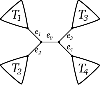
Figure 3: Notation used in the proof of Theorem 31.

The following proposition says that the sort of mixture described in Theorem 31 is possible (assuming the main result of [7]). It is a simple general fact.

Proposition 44.

Let $T_{1},\ldots,T_{4}$ be rooted trees and $R$ and $S$ two trees on the taxon set $\{1,2,3,4\}$. Let $\tilde{R}$ and $\tilde{S}$ be the trees obtained from $R$ and $S$ by attaching tree $T_{i}$ in place of taxon $i$. Now if $R\rightarrowtail S$ then $\tilde{R}\rightarrowtail\tilde{S}$.

Proof.

Let the vector $\underline{y}$ represent the state vector for the terminal taxa on $R$ and $S$ and let $\underline{x_{i}}$ represent the state vector for the tree $T_{i}$. Let $p_{\gamma}^{T}(\underline{z})$ mean the probability of state vector $\underline{z}$ on a tree $T$ with branch lengths $\underline{\gamma}$; $\underline{\gamma}$ will be omitted if understood. The statement $R\rightarrowtail S$ means exactly that there exist $\underline{\gamma_{1}}$, $\underline{\gamma_{2}}$, $\underline{\gamma_{3}}$ and $\alpha$ such that

$$\alpha p_{\underline{\gamma_{1}}}^{R}(\underline{y})+(1-\alpha)p_{\underline{\gamma_{2}}}^{R}(\underline{y})=p_{\underline{\gamma_{3}}}^{S}(\underline{y})$$

for any state vector $\underline{y}$. We observe that

$$p^{\tilde{W}}(\underline{x_{1}},\ldots,\underline{x_{4}})=\sum_{\underline{y}}\,p^{W}(\underline{y})\prod_{i=1}^{4}p^{T_{i}}(\underline{x_{i}}|y_{i})$$

for $W=R,S$, where $p^{T_{i}}(\underline{x_{i}}|y_{i})$ is the probability of state vector $\underline{x_{i}}$ assuming the root of $T_{i}$ is in state $y_{i}$. This implies

$$\begin{split}\alpha p_{\underline{\tilde{\gamma}_{1}}}^{\tilde{R}}(\underline{x_{1}},\ldots,\underline{x_{4}})+(1-\alpha)p_{\underline{\tilde{\gamma}_{2}}}^{\tilde{R}}(&\underline{x_{1}},\ldots,\underline{x_{4}})\\ &=\sum_{\underline{y}}\,\left(\alpha p_{\underline{\gamma_{1}}}^{R}(\underline{y})+(1-\alpha)p_{\underline{\gamma_{2}}}^{R}(\underline{y})\right)\prod_{i=1}^{4}p^{T_{i}}(\underline{x_{i}}|y_{i})\\ &=p_{\underline{\tilde{\gamma}_{3}}}^{\tilde{S}}(\underline{x_{1}},\ldots,\underline{x_{4}})\end{split}$$

where the $\underline{\tilde{\gamma}_{j}}$ are simply the $\underline{\gamma_{j}}$ along with the branch lengths of the $T_{i}$.

∎

For completeness we also record when a two class phylogenetic mixture on a tree can mimic a tree of the same topology under the CFN model.

Proposition 45.

If a two class phylogenetic mixture on a tree mimics a tree of the same topology under the binary symmetric model, then all branch lengths between the two sets must be the same with the possible exception of those for a quartet of adjacent edges sitting inside the tree.

Proof.

Assume a counter-example to Proposition 45: i.e. that there exists a tree $R$ with two branch length sets which differ by more than a quartet of adjacent edges but which mix to mimic a tree of the same topology $S$ under the binary symmetric model. Therefore, there exists a partitioning of $R$ into subtrees $A$, $B$, and $C$ meeting at a node such that there is an edge in each of $A$ and $B$ which differs in terms of branch length between the two sets. Note that if two branch length sets differ on a nontrivial rooted tree, then by induction one can find an induced rooted subtree of size two which differs in terms of branch length between the two branch length sets. Therefore there must be an induced rooted subtree of size two in each of $A$ and $B$ which differs in terms of branch length between the two branch length sets. Number the taxa thus chosen from $A$ with 1 and 2, and the taxa chosen from $B$ with 3 and 4. Label an arbitrary taxon from $C$ with 5. Now consider the induced 5-taxon tree induced by restricting the taxon set to 1 through 5. Label the edges as in Figure 2, and assign (induced) $k_{i}$’s as before.

From the above we can assume (perhaps after renumbering) that $k_{1}\neq 1$ and $k_{3}\neq 1$. By restricting $R$ to the taxon set $1234$ we have by Lemma 34 that $k_{1}=k_{2}^{-1}$ and $k_{3}=k_{4}$ (perhaps after renumbering.) Because $k_{3}\neq 1$, we have $k_{3}\neq k_{4}^{-1}$. Thus using Lemma 34, by restricting to $1534$ we have $k_{1}k_{6}=k_{5}$ and by restricting to $2534$ we have $k_{2}k_{6}=k_{5}$. Therefore $k_{1}=k_{2}=1$, which is a contradiction. ∎

3 Conclusion

We have presented a number of new results which help to clarify when non-identifiable phylogenetic mixtures may pose a problem for reconstruction. However, the message isn’t completely straightforward. The first section shows that the space of site-pattern frequency vectors for phylogenetic mixtures on many quartet trees contains a relatively large non-identifiable region. Furthermore, this non-identifiable region under the CFN model contains site-pattern frequencies for resolved trees with substantial internal branch lengths. Yet, these spaces were constructed using specific trees of extreme branch lengths, raising the question of whether corresponding results hold for more reasonable parameter regimes and “random” sets of trees which one might find from data. Furthermore, we wonder if it is possible to find simple $H$-descriptions of the phylogenetic mixture polytope for larger star trees.

On the other hand, the second section shows generally that phylogenetic mixtures on just two trees may not pose so much of a problem. In particular, our results make progress towards showing that clocklike two class phylogenetic mixtures may be identifiable under further assumptions. We also show that pairs of trees under CFN rates-across-sites mixtures are identifiable. Finally, we show that two class phylogenetic mixtures on a tree cannot “change” the topology too much.

In general, many interesting questions remain and we look forward to seeing further progress in this field.

Acknowledgements

The authors are grateful to Sebastien Roch for helpful discussions on this work, and to the two anonymous referees for their many helpful comments.

References

- [1] E. S. Allman and J. A. Rhodes. The identifiability of tree topology for phylogenetic models, including covarion and mixture models. J. Comput. Biol., 13(5):1101–1113, 2006.
- [2] H. J. Bandelt and A. W. M. Dress. A canonical decomposition theory for metrics on a finite set. Adv. Math., 92:47–105, 1992.
- [3] J. Felsenstein. Inferring Phylogenies. Sinauer Press, Sunderland, MA, 2004.
- [4] E. Gawrilow and M. Joswig. Geometric reasoning with polymake. arXiv:math.CO/0507273, 2005.
- [5] B. Grünbaum. Convex Polytopes. Springer-Verlag, Berlin, 2003.
- [6] Volker Kaibel and Marc E. Pfetsch. Some algorithmic problems in polytope theory. In Algebra, geometry, and software systems, pages 23–47. Springer, Berlin, 2003.
- [7] F. A. Matsen and M. Steel. Phylogenetic mixtures on a single tree can mimic a tree of another topology. arXiv:0704.2260v1 [q-bio.PE], 2007.
- [8] C. A. Meacham. Theoretical and computational considerations of the compatibility of qualitative taxonomic characters. In J. Felsenstein, editor, Numerical taxonomy, volume G1 of NATO ASI Series, pages 304–314. Springer-Verlag, Berlin, 1983.
- [9] E. Mossel and M. Steel. A phase transition for a random cluster model on phylogenetic trees. Math. Biosci., 187(4):189–203, 2004.
- [10] H. Ochman, J. G. Lawrence, and E. A. Groisman. Lateral gene transfer and the nature of bacterial innovation. Nature, 405(6784):299–304, 2000.
- [11] A. Rokas, B. L. Williams, N. King, and S. B. Carroll. Genome-scale approaches to resolving incongruence in molecular phylogenies. Nature, 425(6960):798–804, 2003.
- [12] C. Semple and M. Steel. Phylogenetics, volume 24 of Oxford Lecture Series in Mathematics and its Applications. Oxford University Press, Oxford, 2003.
- [13] C. Simon, L. Nigro, J. Sullivan, K. Holsinger, A. Martin, A. Grapputo, A. Franke, and C. McIntosh. Large differences in substitutional pattern and evolutionary rate of 12S ribosomal RNA genes. Mol Biol Evol, 13(7):923–932, 1996.
- [14] M. A. Steel, L. A. Szekely, and M. D. Hendy. Reconstructing trees when sequence sites evolve at variable rates. J. Comput. Biol., 1(2):153–163, 1994.
- [15] D. Štefankovič and E. Vigoda. Phylogeny of mixture models: Robustness of maximum likelihood and non-identifiable distributions. J. Comput. Biol., 14(2):156–189, 2007.
- [16] G. M. Ziegler. Lectures on Convex Polytopes. Springer-Verlag, Berlin, 1994.