Stability of isentropic viscous shock profiles in the high-Mach number limit

Abstract

By a combination of asymptotic ODE estimates and numerical Evans function calculations, we establish stability of viscous shock solutions of the isentropic compressible Navier–Stokes equations with $\gamma$-law pressure (i) in the limit as Mach number $M$ goes to infinity, for any $\gamma\geq 1$ (proved analytically), and (ii) for $M\geq 2,500$, $\gamma\in[1,2.5]$ (demonstrated numerically). This builds on and completes earlier studies by Matsumura–Nishihara and Barker–Humpherys–Rudd–Zumbrun establishing stability for low and intermediate Mach numbers, respectively, indicating unconditional stability, independent of shock amplitude, of viscous shock waves for $\gamma$-law gas dynamics in the range $\gamma\in[1,2.5]$. Other $\gamma$-values may be treated similarly, but have not been checked numerically. The main idea is to establish convergence of the Evans function in the high-Mach number limit to that of a pressureless, or “infinitely compressible”, gas with additional upstream boundary condition determined by a boundary-layer analysis. Recall that low-Mach number behavior is incompressible.

1 Introduction

The isentropic compressible Navier-Stokes equations in one spatial dimension expressed in Lagrangian coordinates take the form

$$\begin{split}v_{t}-u_{x}&=0,\\ u_{t}+p(v)_{x}&=\left(\frac{u_{x}}{v}\right)_{x},\end{split}$$ (1)

where $v$ is specific volume, $u$ is velocity, and $p$ pressure. We assume an adiabatic pressure law

$$p(v)=a_{0}v^{-\gamma}$$ (2)

corresponding to a $\gamma$-law gas, for some constants $a_{0}>0$ and $\gamma\geq 1$. In the thermodynamical rarified gas approximation, $\gamma>1$ is the average over constituent particles of $\gamma=(n+2)/n$, where $n$ is the number of internal degrees of freedom of an individual particle Ba : $n=3$ ($\gamma=1.66...$) for monatomic, $n=5$ ($\gamma=1.4$) for diatomic gas. For dense fluids, $\gamma$ is typically determined phenomenologically H . In general, $\gamma$ is usually taken within $1\leq\gamma\leq 3$ in models of gas- or fluid-dynamical flow, whether phenomenological or derived by statistical mechanics Sm ; Se.1 ; Se.2 .

It is well known that these equations support viscous shock waves, or asymptotically-constant traveling-wave solutions

$$(v,u)(x,t)=({\hat{v}},{\hat{u}})(x-st),\qquad\lim_{z\to\pm\infty}({\hat{v}},{\hat{u}})(z)=(v,u)_{\pm},$$ (3)

in agreement with physically-observed phenomena. In nature, such waves are seen to be quite stable, even for large variations in pressure between $v_{\pm}$. However, it is a long-standing mathematical question to what extent this is reflected in the continuum-mechanical model (1), that is, for which choice of parameters $(v_{\pm},u_{\pm},\gamma)$ are solutions of (3) time-evolutionarily stable in the sense of PDE; see, for example, the discussions in IO ; BE .

The first result on this problem was obtained by Matsumura and Nishihara in 1985 MN using clever energy estimates on the integrals of perturbations in $v$ and $u$, by which they established stability with respect to the restricted class of perturbations with “zero mass”, i.e., perturbations whose integral is zero, for shocks with sufficiently small amplitude

$$|p(v_{+})-p(v_{-})|\leq C(v_{-},\gamma),$$

with $C\to\infty$ as $\gamma\to 1$, but $C<<\infty$ for $\gamma\neq 1$. There followed a number of works by Liu, Goodman, Szepessy-Xin, and others L.1 ; Go.2 ; SX ; L.2 toward the treatment of general, nonzero mass perturbations; see ZH ; Z.2 ; Z.3 and references therein. A complete result of stability with respect to general $L^{1}\cap H^{3}$ perturbations of small-amplitude shocks of system (1) was finally obtained in 2004 by Mascia and Zumbrun MZ.2 using pointwise semigroup techniques introduced by Zumbrun and Howard ZH ; Z.4 in the strictly parabolic case.

The result of MZ.2 , together with the small-amplitude spectral stability result of Humpherys and Zumbrun HuZ.2 generalizing that of MN , in fact yields stability of small-amplitude shocks of general symmetric hyperbolic-parabolic systems, largely settling the problem of small-amplitude shock stability for continuum mechanical systems.

However, there remains the interesting question of large-amplitude stability. The main result in this direction, following a general strategy proposed in ZH , is a “refined Lyapunov theorem” established by Mascia and Zumbrun MZ.4 ; Z.3 for general symmetric hyperbolic–parabolic systems, stating that linearized and nonlinear $L^{1}\cap H^{3}\to L^{1}\cap H^{3}$ orbital stability (the standard notions of stability) are equivalent to spectral stability, or nonexistence of nonstable (nonnegative real part) eigenvalues of the linearized operator $L$ about the wave, other than the single zero eigenvalue arising through translational invariance of the underlying equations.

This reduces the problem of large-amplitude stability to the study of the associated eigenvalue equation $(L-\lambda)u=0$, a standard analytically and numerically well-posed (boundary value) problem in ODE, which can be attacked by the large body of techniques developed for asymptotic, exact, and numerical study of ODE. In particular, there exist well-developed and efficient numerical algorithms to determine the number of unstable roots for any specific linearized operator $L$, independent of its origins in the PDE setting; see, e.g., Br.1 ; Br.2 ; BrZ ; BDG ; HuZ.2 and references therein. In this sense, the problem of determining stability of any single wave is satisfactorily resolved, or, for that matter, of any compact family of waves. To determine stability of a family of waves across an unbounded parameter regime, however, is another matter. It is this issue that we confront in attempting to decide the stability of general isentropic Navier–Stokes shocks.

As pointed out in ZH ; HuZ.1 , zero-mass stability implies (and in a practical sense is roughly equivalent to) spectral stability. Thus, the original results of Matsumura and Nishida MN imply small-amplitude shock stability for general $\gamma$ and large-amplitude stability as $\gamma\to 1$. Recently, Barker, Humpherys, Rudd, and Zumbrun BHRZ have carried out a numerical Evans function study indicating stability on the large, but still bounded, parameter range $\gamma\in[1,3]$, $1\leq M\leq 3,000$, where $M$ is the Mach number associated with the shock. For discussion of the Evans function, see Section 2.4. Recall that Mach number is an alternative measure of shock strength, with $1$ corresponding to $|p(v_{+})-p(v_{-})|=0$ and $M\to\infty$ corresponding to $|p(v_{+})-p(v_{-})|\to\infty$; see Appendix A, BHRZ , or Section 2.1 below. Mach $3,000$ is far beyond the hypersonic regime $M\sim 10^{1}$ encountered in current aerodynamics. However, the mathematical question of stability across arbitrary $\gamma$, $M$ remains open up to now.

In this paper, we resolve this question, using a combination of asymptotic ODE estimates and Evans function calculations to conclude, first, stability of isentropic Navier–Stokes shocks in the large Mach number limit $M\to\infty$ for any $\gamma\geq 1$, and, second, stability for all $M\geq 2,500$ for $\gamma\in[1,2.5]$ (for $\gamma\in[1,2]$, we obtain in fact stability for $M\geq 500$.) The first result is obtained analytically, the second by a systematic numerical study. Together with the numerical results of BHRZ , this gives convincing numerical evidence of unconditional stability for $\gamma\in[1,2.5]$, independent of shock amplitude. As in BHRZ , our numerical study is not a numerical proof, but contains the necessary ingredients for one; see discussion, Section 6. The restriction to $\gamma\in[1,2.5]$ is an arbitrary one coming from the choice of parameters on which the numerical study BHRZ was carried out; stability for other $\gamma$ can be easily checked as well.

Our method of analysis is straightforward, though somewhat delicate to carry out. Working with the rescaled and conveniently rearranged versions of the equations introduced in BHRZ , we observe that the associated eigenvalue equations converge uniformly as Mach number goes to infinity on a “regular region” $x\leq L$, for any fixed $L>0$, to a limiting system that is well-behaved (hence treatable by the standard methods of MZ.3 ; PZ ; BHRZ ) in the sense that its coefficient matrix converges uniformly exponentially in $x$ to limits at $x=\pm\infty$, but is underdetermined at $x=+\infty$.

On the complementary “singular region” $x\geq L$, the convergence is only pointwise due to a fast “inner structure” featuring rapid variation of the converging coefficient matrices near $x=+\infty$, but the behavior at $x=+\infty$ is of course determinate. Performing a boundary-layer analysis on the singular region and matching across $x=L$, we are able to show convergence of the Evans function of the original system as the Mach number goes to infinity to an Evans function of the limiting system with an appropriately imposed additional condition at $x=+\infty$, upstream of the shock. This reduces the question of stability in the high-Mach number limit to existence or nonexistence of zeroes of the limiting Evans function on $\Re e\lambda\geq 0$, a question that can be resolved by routine numerical computation as in BHRZ , or by energy estimates as in Appendix B.

The limiting system can be recognized as the eigenvalue equation associated with a pressure-less ($\gamma=0$) gas, that is, the “infinitely-compressible” limit one might expect as the Mach number goes to infinity. Recall that behavior in the low Mach number limit is incompressible KM ; KLN ; Ho . However, the upstream boundary condition has to our knowledge no such simple interpretation. Indeed, to carry out the boundary-layer analysis by which we derive this condition is the main technical difficulty of the paper.

Besides their independent interest, the results of this paper seem significant as prototypes for future analyses. Our calculations use some properties specific to the structure of (1). In particular, we make use of surprisingly strong energy estimates carried out in BHRZ in confining unstable eigenvalues to a bounded set independent of shock strength (or Mach number). Also, we use the extremely simple structure of the eigenvalue equation to carry out the key analysis of the eigenvalue flow in the singular region near $x=+\infty$ essentially by hand. However, these appear to be conveniences rather than essential aspects of the analysis. It is our hope that the basic argument structure of this paper together with BHRZ can serve as a blueprint for the study of large-amplitude stability in more general situations.

In particular, we expect that the analysis will carry over to the full (nonisentropic) equations of gas dynamics with ideal gas equation of state, which, formally, decouple in the high-Mach number limit into the equations of isentropic pressureless gas dynamics studied here, augmented with a separate temperature equation governed by simple diffusion/Fourier’s law.

2 Preliminaries

We begin by recalling a number of preliminary steps carried out in BHRZ . Making the standard change of coordinates $x\rightarrow x-st$, we consider instead stationary solutions $(v,u)(x,t)\equiv({\hat{v}},{\hat{u}})(x)$ of

$$\begin{split}v_{t}-sv_{x}-u_{x}&=0,\\ u_{t}-su_{x}+(a_{0}v^{-\gamma})_{x}&=\left(\frac{u_{x}}{v}\right)_{x}.\end{split}$$ (4)

Under the rescaling

$$(x,t,v,u)\rightarrow(-\varepsilon sx,\varepsilon s^{2}t,v/\varepsilon,-u/(\varepsilon s)),$$ (5)

where $\varepsilon$ is chosen so that $0<v_{+}<v_{-}=1$, our system takes the convenient form

$$\begin{split}v_{t}+v_{x}-u_{x}&=0,\\ u_{t}+u_{x}+(av^{-\gamma})_{x}&=\left(\frac{u_{x}}{v}\right)_{x},\end{split}$$ (6)

where $a=a_{0}\varepsilon^{-\gamma-1}s^{-2}$.

2.1 Profile equation

Steady shock profiles of (6) satisfy

$$\begin{split}v^{\prime}-u^{\prime}&=0,\\ u^{\prime}+(av^{-\gamma})^{\prime}&=\left(\frac{u^{\prime}}{v}\right)^{\prime},\end{split}$$

subject to boundary conditions $(v,u)(\pm\infty)=(v_{\pm},u_{\pm})$, or, simplifying,

$$v^{\prime}+(av^{-\gamma})^{\prime}=\left(\frac{v^{\prime}}{v}\right)^{\prime}.$$

Integrating from $-\infty$ to $x$, we get the profile equation

$$v^{\prime}=H(v,v_{+}):=v(v-1+a(v^{-\gamma}-1)),$$ (7)

where $a$ is found by setting $x=+\infty$, thus yielding the Rankine-Hugoniot condition

$$a=-\frac{v_{+}-1}{v_{+}^{-\gamma}-1}=v_{+}^{\gamma}\frac{1-v_{+}}{1-v_{+}^{\gamma}}.$$ (8)

Evidently, $a\to\gamma^{-1}$ in the weak shock limit $v_{+}\to 1$, while $a\sim v_{+}^{\gamma}$ in the strong shock limit $v_{+}\to 0$. The associated Mach number $M$ may be computed as in BHRZ , Appendix A, as

$$M=(\gamma a)^{-1/2}$$ (9)

so that $M\sim\gamma^{-1/2}v_{+}^{-\gamma/2}\to+\infty$ as $v_{+}\to 0$ and $M\to 1$ as $v_{+}\to 1$; that is, the high-Mach number limit corresponds to the limit $v_{+}\to 0$.

2.2 Eigenvalue equations

Linearizing (6) about the profile $({\hat{v}},{\hat{u}})$, we obtain the eigenvalue problem

$$\begin{split}&\lambda v+v^{\prime}-u^{\prime}=0,\\ &\lambda u+u^{\prime}-\left(\frac{h({\hat{v}})}{{\hat{v}}^{\gamma+1}}v\right)^{\prime}=\left(\frac{u^{\prime}}{{\hat{v}}}\right)^{\prime},\end{split}$$ (10)

where

$$h({\hat{v}})=-{\hat{v}}^{\gamma+1}+a(\gamma-1)+(a+1){\hat{v}}^{\gamma}.$$ (11)

We seek nonstable eigenvalues $\lambda\in\{\Re e(\lambda)\geq 0\}\setminus\{0\}$, i.e., $\lambda$ for which (10) possess a nontrivial solution $(v,u)$ decaying at plus and minus spatial infinity. As pointed out in ZH ; HuZ.1 , by divergence form of the equations, such solutions necessarily satisfy $\int_{-\infty}^{+\infty}v(x)dx=\int_{-\infty}^{+\infty}u(x)dx=0$, from which we may deduce that

$$\tilde{u}(x)=\int_{-\infty}^{x}u(z)dz,\quad\tilde{v}(x)=\int_{-\infty}^{x}v(z)dz$$

and their derivatives decay exponentially as $x\rightarrow\infty$. Substituting and then integrating, we find that $(\tilde{u},\tilde{v})$ satisfies the integrated eigenvalue equations (suppressing the tilde)

$$\lambda v+v^{\prime}-u^{\prime}=0,$$ (12a)

$$\lambda u+u^{\prime}-\frac{h({\hat{v}})}{{\hat{v}}^{\gamma+1}}v^{\prime}=\frac{u^{\prime\prime}}{{\hat{v}}}.$$ (12b)

This new eigenvalue problem differs spectrally from (10) only at $\lambda=0$, hence spectral stability of (10) is equivalent to spectral stability of (12). Moreover, since (12) has no eigenvalue at $\lambda=0$, one can expect more uniform stability estimates for the integrated equations in the vicinity of $\lambda=0$ MN ; Go.1 ; ZH .

2.3 Preliminary estimates

The following estimates established in BHRZ indicate the suitability of the rescaling chosen in Section 2.1. For completeness, we prove these in Appendix A.

Proposition 1 (BHRZ )

For each $\gamma\geq 1$, $0<v_{+}\leq 1$, (7) has a unique (up to translation) monotone decreasing solution $\hat{v}$ decaying to its endstates with a uniform exponential rate, independent of $v_{+}$, $\gamma$. In particular, for $0<v_{+}\leq\frac{1}{12}$ and $\hat{v}(0):=v_{+}+\frac{1}{12}$,

$$|{\hat{v}}(x)-v_{+}| \leq\Big{(}\frac{1}{12}\Big{)}e^{-\frac{3x}{4}}\quad x\geq 0,$$ (13a)

$$|{\hat{v}}(x)-v_{-}| \leq\Big{(}\frac{1}{4}\Big{)}e^{\frac{x+12}{2}}\quad x\leq 0.$$ (13b)

Proposition 2 (BHRZ )

Nonstable eigenvalues $\lambda$ of (12), i.e., eigenvalues with nonnegative real part, are confined for any $0<v_{+}\leq 1$ to the region

$$\Re e(\lambda)+|\Im m(\lambda)|\leq\Big{(}\sqrt{\gamma}+\frac{1}{2}\Big{)}^{2}.$$ (14)

2.4 Evans function formulation

Following BHRZ , we may express (12) concisely as a first-order system

$$W^{\prime}=A(x,\lambda)W,$$ (15)

$$A(x,\lambda)=\begin{pmatrix}0&\lambda&1\\ 0&0&1\\ \lambda{\hat{v}}&\lambda{\hat{v}}&f({\hat{v}})-\lambda\end{pmatrix},\quad W=\begin{pmatrix}u\\ v\\ v^{\prime}\end{pmatrix},\quad\prime=\frac{d}{dx},$$ (16)

where

$$f({\hat{v}})={\hat{v}}-{\hat{v}}^{-\gamma}h({\hat{v}})=2{\hat{v}}-a(\gamma-1){\hat{v}}^{-\gamma}-(a+1),$$ (17)

with $h$ as in (11) and $a$ as in (8), or, equivalently,

$$f({\hat{v}})=2{\hat{v}}-(\gamma-1)\Big{(}\frac{1-v_{+}}{1-v_{+}^{\gamma}}\Big{)}\Big{(}\frac{v_{+}}{{\hat{v}}}\Big{)}^{\gamma}-\Big{(}\frac{1-v_{+}}{1-v_{+}^{\gamma}}\Big{)}v_{+}^{\gamma}-1.$$ (18)

Eigenvalues of (12) correspond to nontrivial solutions $W$ for which the boundary conditions $W(\pm\infty)=0$ are satisfied. Because $A(x,\lambda)$ as a function of ${\hat{v}}$ is asymptotically constant in $x$, the behavior near $x=\pm\infty$ of solutions of (16) is governed by the limiting constant-coefficient systems

$$W^{\prime}=A_{\pm}(\lambda)W,\qquad A_{\pm}(\lambda):=A(\pm\infty,\lambda),$$ (19)

from which we readily find on the (nonstable) domain $\Re e\lambda\geq 0$, $\lambda\neq 0$ of interest that there is a one-dimensional unstable manifold $W_{1}^{-}(x)$ of solutions decaying at $x=-\infty$ and a two-dimensional stable manifold $W_{2}^{+}(x)\wedge W_{3}^{+}(x)$ of solutions decaying at $x=+\infty$, each of which may be chosen analytically in $\lambda$. With additional care, these may be extended analytically to the whole set $\Re e\lambda\geq 0$, i.e., to $\lambda=0$ GZ . Defining the Evans function $D$ associated with operator $L$ as the analytic function

$$D(\lambda):=\det(W_{1}^{-}W_{2}^{+}W_{3}^{+})_{\mid x=0},$$ (20)

we find that eigenvalues of $L$ correspond to zeroes of $D$ both in location and multiplicity; see, e.g., AGJ ; GZ ; MZ.3 ; Z.3 for further details.

Equivalently, following PW ; BHRZ , we may express the Evans function as

$$D(\lambda)=\big{(}\widetilde{W}_{1}^{+}\cdot W_{1}^{-}\big{)}_{\mid x=0},$$ (21)

where $\widetilde{W}_{1}^{+}(x)$ spans the one-dimensional unstable manifold of solutions decaying at $x=+\infty$ (necessarily orthogonal to the span of $W_{2}^{+}(x)$ and $W_{3}^{+}(x)$) of the adjoint eigenvalue ODE

$$\widetilde{W}^{\prime}=-A(x,\lambda)^{*}\widetilde{W}.$$ (22)

The simpler representation (21) is the one that we shall use here.

3 Description of the main results

We can now state precisely our main results.

3.1 Limiting equations

Under the strategic rescaling (5), both profile and eigenvalues equations converge pointwise as $v_{+}\to 0$ to limiting equations at $v_{+}=0$. The limiting profile equation (the limit of (7)) is evidently

$$v^{\prime}=v(v-1),$$ (23)

with explicit solution

$$\hat{v}_{0}(x)=\frac{1-\tanh(x/2)}{2},$$ (24)

while the limiting eigenvalue system (the limit of (16)) is

$$W^{\prime}=A^{0}(x,\lambda)W,$$ (25)

$$A^{0}(x,\lambda)=\begin{pmatrix}0&\lambda&1\\ 0&0&1\\ \lambda{\hat{v}}_{0}&\lambda{\hat{v}}_{0}&f_{0}({\hat{v}}_{0})-\lambda\end{pmatrix},$$ (26)

where

$$f_{0}({\hat{v}}_{0})=2{\hat{v}}_{0}-1=-\tanh(x/2).$$ (27)

Indeed, this convergence is uniform on any interval $\hat{v}_{0}\geq\epsilon>0$, or, equivalently, $x\leq L$, for $L$ any positive constant, where the sequence is therefore a regular perturbation of its limit. We will call $x\in(-\infty,L]$ the “regular region” or “regular side”. For $\hat{v}_{0}\to 0$ on the other hand, or $x\to\infty$, the limit is less well-behaved, as may be seen by the fact that $\partial f/\partial\hat{v}\sim\hat{v}^{-1}$ as $\hat{v}\to v_{+}$, a consequence of the appearance of $\big{(}\frac{v_{+}}{\hat{v}}\big{)}$ in the expression (18) for $f$. Similarly, in contrast to $\hat{v}$, $A(x,\lambda)$ does not converge to $A_{+}(\lambda)$ as $x\to+\infty$ with uniform exponential rate independent of $v_{+}$, $\gamma$, but rather as $C\hat{v}^{-1}e^{-x/2}$. We call $x\in[L,+\infty)$ therefore the “singular region ” or “singular side”. (This is not a singular perturbation in the usual sense but a weaker type of singularity, at least as we have framed the problem here.)

3.2 Limiting Evans function

We should now like to define a limiting Evans function following the asymptotic Evans function framework introduced in PZ and establish convergence to this function in the $v_{+}\to 0$ limit, thus reducing the stability problem as $v_{+}\to 0$ to the study of the (fixed) limiting Evans function. However, we face certain difficulties due to the (mild) singularity of the limit, as can be seen even at the first step of defining an Evans function for the limiting system.

For, the limiting coefficient matrix

$$A^{0}_{+}(\lambda):=A^{0}(+\infty,\lambda)=\begin{pmatrix}0&\lambda&1\\ 0&0&1\\ 0&0&-1-\lambda\end{pmatrix}$$ (28)

is nonhyperbolic (in ODE sense) for all $\lambda$, having eigenvalues $0,0,-1-\lambda$; in particular, the stable manifold drops to dimension one in the limit $v_{+}\to 0$. Thus, the subspace in which $W_{2}^{+}$ and $W_{3}^{+}$ should be initialized at $x=+\infty$ is not self-determined by (28), but must be deduced by a careful study of the double limit $v_{+}\to 0$, $x\to+\infty$. But, the computation

$$\lim_{v_{+}\to 0}A(+\infty,\lambda)=\begin{pmatrix}0&\lambda&1\\ 0&0&1\\ 0&0&-\gamma-\lambda\end{pmatrix}\neq A^{0}_{+}(\lambda)=\lim_{x\to\infty}\lim_{v_{+}\to 0}A(x,\lambda)$$ (29)

shows that these limits do not commute, except in the special case $\gamma=1$ already treated in MN by other methods.

The rigorous treatment of this issue is the main work of the paper. However, the end result can be easily motivated on heuristic grounds. A study of $\lim_{v_{+}\to 0}A(+\infty,\lambda)$ on the set $\Re e\lambda\geq 0$ of interest reveals that eigenmodes decouple into a single “fast” (stable subspace) decaying mode $(*,*,1)^{T}$ associated with eigenvalue $-\gamma-\lambda$ of strictly negative real part and a two-dimensional (center) subspace of neutral modes $(r,0)^{T}$ associated with Jordan block $\begin{pmatrix}0&\lambda\\ 0&0\end{pmatrix},$ of which there is only a single genuine eigenvector $(1,0,0)^{T}$. For $v_{+}$ small, therefore, $A_{+}(\lambda)$ has also a single fast, decaying, eigenmode with eigenvalue near $-\gamma-1$ and two slow eigenmodes with eigenvalues near zero, one decaying and the other growing (recall, Section 2.4, that the stable subspace of $A_{+}$ has dimension two for $\Re e\lambda\geq 0$, $\lambda\neq 0$ and the unstable subspace dimension one).

Focusing on the single slow decaying eigenvector of $A_{+}$, and considering its limiting behavior as $v_{+}\to 0$, we see immediately that it must converge in direction to $\pm(1,0,0)^{T}$. For, the sequence of direction vectors, since continuously varying and restricted to a compact set, has a nonempty, connected set of accumulation points, and these must be eigenvectors of $\lim_{v_{+}\to 0}A_{+}$ with eigenvalues near zero. Since $\pm(1,0,0)^{T}$ are the unique candidates, we obtain the result. Indeed, both growing and decaying slow eigenmodes must converge to this common direction, making the limiting analysis trivial.

The same argument shows that $\pm(1,0,0)^{T}$ is the limiting direction of the slow stable eigenmode of $A^{0}(x,\lambda)$ as $x\to+\infty$, that is, in the alternate limit $\lim_{x\to\infty}\lim_{v_{+}\to 0}A(x,\lambda)$. That is, $V_{2}^{+}:=(1,0,0)^{T}$ is the common limit of the slow decaying eigenmode in either of the two alternative limits $\lim_{v_{+}\to 0}A_{+}$ and $\lim_{v_{+}\to 0}A_{+}$; it thus seems a reasonable choice to use this limiting slow direction to define an Evans function for the limiting system (26). On the other hand, the stable eigenmode

$$V_{3}:=(a^{-1}(\lambda/a+1),a^{-1},1)^{T},$$

$a=-1-\lambda$, of $A^{0}_{+}$ is forced on us by the system itself, independent of the limiting process.

Combining these two observations, we require that solutions $W^{0+}_{2}$ and $W^{0+}_{3}$ of the limiting eigenvalue system (26) lie asympotically in directions $V_{2}$ and $V_{3}$, respectively, thus determining a limiting, or “reduced” Evans function

$$D^{0}(\lambda):=\det(W_{1}^{0-}W_{2}^{0+}W_{3}^{0+})_{\mid x=0},$$ (30)

or alternatively

$$D^{0}(\lambda)=\big{(}\widetilde{W}_{1}^{0+}\cdot W_{1}^{0-}\big{)}_{\mid x=0},$$ (31)

with $\widetilde{W}_{1}^{0+}$ defined analogously as a solution of the adjoint limiting system lying asymptotically at $x=+\infty$ in direction

$$\widetilde{V}_{1}:=(0,1,\bar{a}^{-1})^{T}=(0,1,(1+\bar{\lambda})^{-1})^{T}$$ (32)

orthogonal to the span of $V_{2}$ and $V_{3}$, where “ $\bar{}$ ” denotes complex conjugate. (The prescription of $W_{1}^{0-}$ in the regular region is straightforward: it must lie on the one-dimensional unstable manifold of $A_{-}^{0}$ as in the $v_{+}>0$ case.)

3.3 Physical interpretation

Alternatively, the limiting equations may be derived by taking a formal limit as $v_{+}\to 0$ of the rescaled equations (6), recalling that $a\sim v_{+}^{\gamma}$, to obtain a limiting evolution equation

$$\begin{split}v_{t}+v_{x}-u_{x}&=0,\\ u_{t}+u_{x}&=\left(\frac{u_{x}}{v}\right)_{x}\end{split}$$ (33)

corresponding to a pressure-less gas, or $\gamma=0$, then deriving profile and eigenvalue equations from (33) in the usual way. This gives some additional insight on behavior, of which we make important mathematical use in Appendix B. Physically, it has the interpretation that, in the high-Mach number limit $v_{+}\to 0$, effects of pressure are concentrated near $x=+\infty$ on the infinite-density side, as encoded in the special upstream boundary condition $(u,u^{\prime},v,v^{\prime})\to c(1,0,0,0)$ as $x\to+\infty$ for the integrated eigenvalue equation, which may be seen to be equivalent to the conditions imposed on $W_{j}^{+}$ in the previous subsection.

3.4 Analytical results

Defining $D^{0}$ as in (30)–(31), we have the following main theorems.

Theorem 3.1

For $\lambda$ in any compact subset of $\Re e\lambda\geq 0$, $D(\lambda)$ converges uniformly to $D^{0}(\lambda)$ as $v_{+}\to 0$.

Corollary 1

For any compact subset $\Lambda$ of $\Re e\lambda\geq 0$, $D$ is nonvanishing on $\Lambda$ for $v_{+}$ sufficiently small if $D^{0}$ is nonvanishing on $\Lambda$, and is nonvanishing on the interior of $\Lambda$ only if $D^{0}$ is nonvanishing there.

Proof

Standard properties of uniform limit of analytic functions.

Corollary 2

Isentropic Navier–Stokes shocks are stable in the high-Mach number limit $v_{+}\to 0$ if $D^{0}$ is nonvanishing on the wedge

$$\Lambda:\Re e(\lambda)+|\Im m(\lambda)|\leq\Big{(}\sqrt{\gamma}+\frac{1}{2}\Big{)}^{2},\quad\Re e\lambda\geq 0$$ (34)

and only if $D^{0}$ is nonvanishing on the interior of $\Lambda$.

Proof

Corollary 1 together with Proposition 2.

Remark 1

Likewise, on any compact subset of $\Re e\lambda\geq 0$, $|D|$ is uniformly bounded from zero for $v_{+}$ sufficiently small ($M$ sufficiently large) if and only if $|D^{0}|$ is uniformly bounded from zero. Thus, isentropic Navier–Stokes shocks are “uniformly stable” for sufficiently small $v_{+}$, in the sense that $|D|$ is bounded from below independent of $v_{+}$, if and only if $D^{0}$ is nonvanishing on $\Lambda$ as defined in (34).

The following result completes our abstract stability analysis. The proof, given in Appendix B, is by an energy estimate analogous to that of MN .

Proposition 3

The limiting Evans function $D^{0}$ is nonzero on $\Re e\lambda\geq 0$.

Corollary 3

For any $\gamma\geq 1$, isentropic Navier–Stokes shocks are stable for Mach number $M$ sufficiently large (equivalently, $v_{+}$ sufficiently small).

3.5 Numerical computations

Unfortunately, the energy estimate used to establish 3, though mathematically elegant, yields only the stated, abstract result and not quantitative estimates. A simpler and more general approach, that does yield quantitative information, is to compute the reduced Evans function numerically. We carry out this by-now routine numerical computation using the methods of BHRZ . Specifically, we map a semicircle $\partial(\{\Re e\lambda\geq 0\}\cap\{|\lambda|\leq 10\})$ enclosing $\Lambda$ for $\gamma\in[1,3]$ by $D^{0}$ and compute the winding number of its image about the origin to determine the number of zeroes of $D^{0}$ within the semicircle, and thus within $\Lambda$. For details of the numerical algorithm, see BHRZ ; BrZ ; HuZ.1 .

The result is displayed in Figure 1, clearly indicating stability. More precisely, the minimum of $|D|$ on the semicircle is found to be $\approx 0.2433$. Together with Rouchés Theorem, this gives explicit bounds on the size of the Mach number for which shocks are stable, as displayed in Table 1, Section 6: specifically, $M\geq 50$ for $\gamma\in[1,2]$, $M\geq 2,400$ for $\gamma\in[2,2.5]$, and $M\geq 13,000$ for $\gamma\in[2.5,3]$, all corresponding approximately to $v_{+}=10^{-3}$. In Figure 2, we superimpose on the image of the semicircle by $D^{0}$ its (again numerically computed) image by the full Evans function $D$, for a monatomic gas $\gamma=1.66...$ at successively higher Mach numbers $v_{+}=$1e-1,1e-2,1e-3,1e-4,1e-5,1e-6, graphically demonstrating the convergence of $D$ to $D^{0}$ as $v_{+}$ approaches zero.

Indeed, we can see a great deal more from Figure 2. For, note that the displayed contours are, to the scale visible by eye, “monotone” in $v_{+}$, or nested, one within the other (they do not appear so at smaller scales). Thus, lower-Mach number contours are essentially “trapped” within higher-Mach number contours, with the worst-case, outmost contour corresponding to the limiting Evans function $D^{0}$. From this observation, we may conclude with confidence stability down to the smallest value $M\approx 5.5$ displayed in the figure, corresponding (see Table 2) to $v_{+}=10^{-1}$. That is, a great deal of topological information is encoded in the analytic family of Evans functions indexed by $v_{+}$, from which stability may be deduced almost by inspection. Behavior for other $\gamma\in[0,3]$ is similar. See, for example, the case $\gamma=3$ displayed in Figure 4, which is virtually identical to Figure 2.

Such topological information does not seem to be available from other methods of investigating stability such as direct discretation of the linearized operator about the wave KL or studies based on linearized time-evolution or power methods BB ; BMFC . This represents in our view a significant advantage of the Evans function formulation.

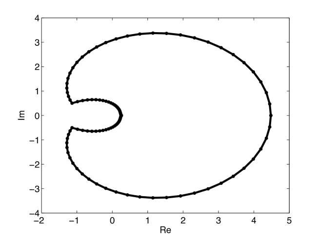
Figure 1: The image of the semi-circular contour via the Evans function for the reduced system. Note that the winding number of this graph is zero. Hence, there are no unstable eigenvalues in the semi-circle.

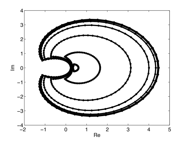
Figure 2: Convergence to the limiting Evans function as $v_{+}\to 0$ for a monatomic gas, $\gamma=1.66...$. The contours depicted, going from inner to outer, are images of the semicircle under $D$ for $v_{+}=$1e-1,1e-2,1e-3,1e-4,1e-5,1e-6. The outermost contour is the image under $D^{0}$, which is nearly indistinguishable from the image for $v_{+}=$1e-6.

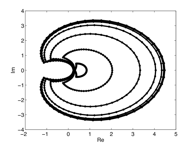
Figure 3: Convergence to the limiting Evans function as $v_{+}\to 0$ for $\gamma=1$. The contours depicted, going from inner to outer, are images of the semicircle under $D$ for $v_{+}=$1e-1,1e-2,1e-3,1e-4,1e-5,1e-6. The outermost contour is the image under $D^{0}$, which is nearly indistinguishable from the image for $v_{+}=$1e-6.

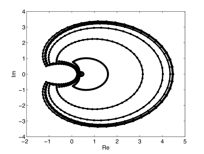
Figure 4: Convergence to the limiting Evans function as $v_{+}\to 0$ for $\gamma=3$. The contours depicted, going from inner to outer, are images of the semicircle under $D$ for $v_{+}=$1e-1,1e-2,1e-3,1e-4,1e-5,1e-6. The outermost contour is the image under $D^{0}$, which is nearly indistinguishable from the image for $v_{+}=$1e-6.

Remark 2

Recall that the Evans function is not determined uniquely, but only up to a nonvanishing analytic factor AGJ ; GZ . The simple contour structure in Figure 2 is thus partly due to a favorable choice of $D$ induced by the initialization at $\pm\infty$ by Kato’s ODE Kato , as described in BrZ ; HuZ.2 ; BHRZ . A canonical algorithm for tracking bases of evolving subspaces, this in some sense minimizes “action”; see HSZ for further discussion.

Remark 3

Note that the limiting equations, and the limiting Evans function $D^{0}$ are both independent of $\gamma$. To study high-Mach number stability for $\gamma>3$, therefore, requires only to examine $D^{0}$ on successively larger semicircles. Thus, our methods in combination with the those of BHRZ , allow us to determine stability in principle over any bounded interval in $\gamma$, for $\gamma>1$ and for all Mach numbers $M\geq 1$.

Remark 4

As Figure 2 suggests, an alternative method for determining stability, without reference to $D^{0}$, is to compute the full Evans function for sufficiently high Mach number. That is, nonvanishing of $D^{0}$, and thus stability of sufficiently high Mach number shocks for $\gamma\in[1,3]$, can already be concluded by large-but-finite Mach number study of BHRZ together with the fact that a limit $D\to D^{0}$ exists (see also Remark 1).

3.6 Conclusions

The analytical result of Corollary 3 guarantees stability for $\gamma\geq 1$, $M$ sufficiently large. For $\gamma\in[1,2.5]$, our numerical results indicate stability for $M\geq 2,500$ by a crude Rouche bound, and indeed much lower if further structure is taken into account. Together with the small and intermediate Mach number studies of MN ; BHRZ for $M\leq 3,000$, this yields unconditional stability of isentropic Navier–Stokes shocks for $\gamma\in[1,2.5]$ and $M\geq 1$. There is no inherent restriction to $\gamma\in[1,2.5]$; as discussed in Remark 3, numerical computations can be carried out for any value of $\gamma$ to determine stability (or instability) for all $M\geq 1$. Indeed, our method of analysis indicates that the large-$\gamma$ limit is quite analogous to the high-Mach number limit $v_{+}\to 0$, suggesting the possibility to establish still more general results encompassing all $\gamma\geq 1$, $M\geq 1$.

Our numerical results reveal also an unexpected “universality” of behavior in the high-Mach number regime, beyond just convergence to the limiting system. Namely, we see (cf. Figures 2 and 4) that behavior for a given $v_{+}$ is virtually independent of the value of $\gamma$. This also indicates that $v_{+}$ and not $M$ is the more useful measure of shock strength in this regime.

4 Boundary-layer analysis

We now carry out the main work of the paper, analyzing the flow of (16) in the singular region. Our starting point is the observation that

$$A(x,\lambda)=\begin{pmatrix}0&\lambda&1\\ 0&0&1\\ \lambda\hat{v}&\lambda\hat{v}&f(\hat{v})-\lambda\end{pmatrix}$$ (35)

is approximately block upper-triangular for $\hat{v}$ sufficiently small, with diagonal blocks $\begin{pmatrix}0&\lambda\\ 0&0\\ \end{pmatrix}$ and $\begin{pmatrix}f(\hat{v})-\lambda\end{pmatrix}$ that are uniformly spectrally separated on $\Re e\lambda\geq 0$, as follows by

$$f(\hat{v})\leq 2\hat{v}-1\leq-1/2.$$ (36)

We exploit this structure by a judicious coordinate change converting (16) to a system in exact upper triangular form, for which the decoupled “slow” upper lefthand $2\times 2$ block undergoes a regular perturbation that can be analyzed by standard tools introduced in PZ . Meanwhile, the fast, lower righthand $1\times 1$ block, since scalar, may be solved exactly.

The global structure of this argument loosely follows the general strategy of PZ of first decoupling fast and slow modes, then treating slow modes by regular perturbation methods. However, there are interesting departures that may be of use in other degenerate situations. First, we only partially decouple the system, to block-triangular rather than block-diagonal form as in more standard cases, and second, we introduce a more stable method of block-reduction taking account of usually negligible derivative terms in the definition of block-triangularizing transformations, which, if ignored, would in this case lead to unacceptably large errors.

4.1 Preliminary transformation

We first block upper-triangularize by a static (constant) coordinate transformation the limiting matrix

$$A_{+}=A(+\infty,\lambda)=\begin{pmatrix}0&\lambda&1\\ 0&0&1\\ \lambda v_{+}&\lambda v_{+}&f(v_{+})-\lambda\end{pmatrix}$$ (37)

at $x=+\infty$ using special block lower-triangular transformations

$$R_{+}:=\begin{pmatrix}I&0\\ \lambda v_{+}\theta_{+}&1\\ \end{pmatrix},\qquad L_{+}:=R_{+}^{-1}=\begin{pmatrix}I&0\\ -\lambda v_{+}\theta_{+}&1\\ \end{pmatrix},$$ (38)

where $I$ denotes the $2\times 2$ identity matrix and $\theta_{+}\in\mathbb{C}^{1\times 2}$ is a $1\times 2$ row vector.

Lemma 1

On any compact subset of $\Re e\lambda\geq 0$, for each $v_{+}>0$ sufficiently small, there exists a unique $\theta_{+}=\theta_{+}(v_{+},\lambda)$ such that $\hat{A}_{+}:=L_{+}A_{+}R_{+}$ is upper block-triangular,

$$\hat{A}_{+} =\begin{pmatrix}\lambda(J+v_{+}{1\!\!1}\theta_{+})&{1\!\!1}\\ 0&f(\hat{v})-\lambda-\lambda v_{+}\theta_{+}{1\!\!1}\\ \end{pmatrix},$$ (39)

where $J=\begin{pmatrix}0&1\\ 0&0\end{pmatrix}$ and ${1\!\!1}=\begin{pmatrix}1\\ 1\\ \end{pmatrix}$, satisfying a uniform bound

$$|\theta_{+}|\leq C.$$ (40)

Proof

Setting the $2-1$ block of $\hat{A}_{+}$ to zero, we obtain the matrix equation

$$\theta_{+}(aI-\lambda J)=-{1\!\!1}^{T}+\lambda v_{+}\theta_{+}{1\!\!1}\theta_{+},$$

where $a=f(v_{+})-\lambda$, or, equivalently, the fixed-point equation

$$\theta_{+}=(aI-\lambda J)^{-1}\Big{(}-{1\!\!1}^{T}+\lambda v_{+}\theta_{+}{1\!\!1}\theta_{+}\Big{)}.$$ (41)

By $\det(aI-\lambda J)=a^{2}\neq 0$, $(aI-\lambda J)^{-1}$ is uniformly bounded on compact subsets of $\Re e\lambda\geq 0$ (indeed, it is uniformly bounded on all of $\Re e\lambda\geq 0$), whence, for $|\lambda|$ bounded and $v_{+}$ sufficiently small, there exists a unique solution by the Contraction Mapping Theorem, which, moreover, satisfies (40).

4.2 Dynamic triangularization

Defining now $Y:=L_{+}W$ and

$$\hat{A}(x,\lambda) =L_{+}A(x,\lambda)R_{+}(x,\lambda)$$ (42)

$$=\begin{pmatrix}\\ \lambda(J+v_{+}{1\!\!1}\theta_{+})&{1\!\!1}\\ \lambda(\hat{v}-v_{+}){1\!\!1}^{T}-\lambda v_{+}(f(\hat{v})-f(v_{+}))\theta_{+}&f(\hat{v})-\lambda-\lambda v_{+}\theta_{+}{1\!\!1}\\ \end{pmatrix},$$

we have converted (16) to an asymptotically block upper-triangular system

$$Y^{\prime}=\hat{A}(x,\lambda)Y,$$ (43)

with $\hat{A}_{+}=\hat{A}(+\infty,\lambda)$ as in (39). Our next step is to choose a dynamic transformation of the same form

$$\tilde{R}:=\begin{pmatrix}I&0\\ \tilde{\Theta}&1\\ \end{pmatrix},\qquad\tilde{L}:=\tilde{R}^{-1}=\begin{pmatrix}I&0\\ -\tilde{\Theta}&1\\ \end{pmatrix},$$ (44)

converting (43) to an exactly block upper-triangular system, with $\tilde{\Theta}$ uniformly exponentially decaying at $x=+\infty$: that is, a regular perturbation of the identity.

Lemma 2

On any compact subset of $\Re e\lambda\geq 0$, for $L$ sufficiently large and each $v_{+}>0$ sufficiently small, there exists a unique $\Theta=\Theta_{+}(x,\lambda,v_{+})$ such that $\tilde{A}:=\tilde{L}\hat{A}(x,\lambda)\tilde{R}+\tilde{L}^{\prime}\tilde{R}$ is upper block-triangular,

$$\tilde{A} =\begin{pmatrix}\lambda(J+v_{+}{1\!\!1}\theta_{+})+{1\!\!1}\tilde{\Theta}&{1\!\!1}\\ 0&f(\hat{v})-\lambda-\lambda\theta_{+}{1\!\!1}-\tilde{\Theta}{1\!\!1}\\ \end{pmatrix},$$ (45)

and $\tilde{\Theta}(L)=0$, satisfying a uniform bound

$$|\tilde{\Theta}(x,\lambda,v_{+})|\leq Ce^{-\eta x},\qquad\eta>0,\,x\geq L,$$ (46)

independent of the choice of $L$, $v_{+}$.

Proof

Setting the $2-1$ block of $\tilde{A}$ to zero and computing

$$\tilde{L}^{\prime}\tilde{R}=\begin{pmatrix}0&0\\ -\tilde{\Theta}^{\prime}&0\end{pmatrix}\begin{pmatrix}I&0\\ \tilde{\Theta}&I\end{pmatrix}=\begin{pmatrix}0&0\\ -\tilde{\Theta}^{\prime}&0,\end{pmatrix}$$

we obtain the matrix equation

$$\tilde{\Theta}^{\prime}-\tilde{\Theta}\big{(}aI-\lambda(J+v_{+}{1\!\!1}\theta_{+})\big{)}=\zeta+\tilde{\Theta}{1\!\!1}\tilde{\Theta},$$ (47)

where the forcing term

$$\zeta:=-\lambda(\hat{v}-v_{+}){1\!\!1}^{T}+\lambda v_{+}(f(\hat{v})-f(v_{+}))\theta_{+}$$

by derivative estimate $df/d\hat{v}\leq C\hat{v}^{-1}$ together with the Mean Value Theorem is uniformly exponentially decaying:

$$|\zeta|\leq C|\hat{v}-v_{+}|\leq C_{2}e^{-\eta x},\qquad\eta>0.$$ (48)

Initializing $\tilde{\Theta}(L)=0$, we obtain by Duhamel’s Principle/Variation of Constants the representation (supressing the argument $\lambda$)

$$\tilde{\Theta}(x)=\int_{L}^{x}S^{y\to x}(\zeta+\tilde{\Theta}{1\!\!1}\tilde{\Theta})(y)\,dy,$$ (49)

where $S^{y\to x}$ is the solution operator for the homogeneous equation

$$\tilde{\Theta}^{\prime}-\tilde{\Theta}\big{(}aI-\lambda(J+v_{+}{1\!\!1}\theta_{+})\big{)}=0,$$

or, explicitly,

$$S^{y\to x}=e^{\int_{y}^{x}a(y)dy}e^{-\lambda(J+v_{+}{1\!\!1}\theta_{+})(x-y)}.$$

For $|\lambda|$ bounded and $v_{+}$ sufficiently small, we have by matrix perturbation theory that the eigenvalues of $-\lambda(J+v_{+}{1\!\!1}\theta_{+})$ are small and the entries are bounded, hence

$$|e^{-\lambda(J+v_{+}{1\!\!1}\theta_{+})z}|\leq Ce^{\epsilon z}$$

for $z\geq 0$. Recalling the uniform spectral gap $\Re ea=f(\hat{v})-\Re e\lambda\leq-1/2$ for $\Re e\lambda\geq 0$, we thus have

$$|S^{y\to x}|\leq Ce^{\eta(x-y)}$$ (50)

for some $C$, $\eta>0$. Combining (48) and (50), we obtain

$$\Big{|}\int_{L}^{x}S^{y\to x}\zeta(y)\,dy\Big{|} \leq\int_{L}^{x}C_{2}e^{-\eta(x-y)}e^{-(\eta/2)y}dy$$ (51)

$$=C_{3}e^{-(\eta/2)x}.$$

Defining $\tilde{\Theta}(x)=:\tilde{\theta}(x)e^{-(\eta/2)x}$ and recalling (49) we thus have

$$\tilde{\theta}(x)=f+e^{(\eta/2)x}\int_{L}^{x}S^{y\to x}e^{-\eta y}\tilde{\theta}{1\!\!1}\tilde{\theta}(y)\,dy,$$ (52)

where $f:=e^{(\eta/2)x}\int_{L}^{x}S^{y\to x}\zeta(y)\,dy$ is uniformly bounded, $|f|\leq C_{3}$, and $e^{(\eta/2)x}\int_{L}^{x}S^{y\to x}e^{-\eta y}\tilde{\theta}{1\!\!1}\tilde{\theta}(y)\,dy$ is contractive with arbitrarily small contraction constant $\epsilon>0$ in $L^{\infty}[L,+\infty)$ for $|\tilde{\theta}|\leq 2C_{3}$ for $L$ sufficiently large, by the calculation

$$\Big{|}e^{(\eta/2)x}\int_{L}^{x}S^{y\to x}e^{-\eta y}\tilde{\theta}_{1}{1\!\!1}\tilde{\theta}_{1}(y)-e^{(\eta/2)x}\int_{L}^{x}S^{y\to x}e^{-\eta y}\tilde{\theta}_{2}{1\!\!1}\tilde{\theta}_{2}(y)\Big{|}$$

$$\qquad\qquad\leq\Big{|}e^{(\eta/2)x}\int_{L}^{x}Ce^{-\eta(x-y)}e^{-\eta y}\,dy\Big{|}\|\tilde{\theta}_{1}-\tilde{\theta}_{2}\|_{\infty}\max_{j}\|\tilde{\theta}_{j}\|_{\infty}$$

$$\qquad\qquad\leq e^{-(\eta/2)L}\Big{|}\int_{L}^{x}Ce^{-(\eta/2)(x-y)}\,dy\Big{|}\|\tilde{\theta}_{1}-\tilde{\theta}_{2}\|_{\infty}\max_{j}\|\tilde{\theta}_{j}\|_{\infty}$$

$$\qquad\qquad=C_{3}e^{-(\eta/2)L}\|\tilde{\theta}_{1}-\tilde{\theta}_{2}\|_{\infty}\max_{j}\|\tilde{\theta}_{j}\|_{\infty}.$$

It follows by the Contraction Mapping Principle that there exists a unique solution $\tilde{\theta}$ of fixed point equation (52) with $|\tilde{\theta}(x)|\leq 2C_{3}$ for $x\geq L$, or, equivalently (redefining the unspecified constant $\eta$), (46).

Remark 5

The above calculation is the most delicate part of the analysis, and the main technical point of the paper. The interested reader may verify that a “quasi-static” transformation treating term $\tilde{\Theta}^{\prime}$ in (47) as an error, as is typically used in situations of slowly-varying coefficients (see for example MZ.3 ; PZ ), would lead to unnaceptable errors of magnitude

$$O(|f(\hat{v}))^{\prime}||\hat{v}-v_{+}|)=O(|df/d\hat{v})||\hat{v}-v_{+}|)=O(|\hat{v}|^{-1}|\hat{v}-v_{+}|).$$

One may think of the exact ODE solution (44) as “averaging” the effects of rapidly-varying coefficients by integration of (47).

4.3 Fast/Slow dynamics

Making now the further change of coordinates

$$Z=\tilde{L}Y$$

and computing

$$(\tilde{L}Y)^{\prime}=\tilde{L}Y^{\prime}+\tilde{L}^{\prime}Y =(\tilde{L}A_{+}+\tilde{L}^{\prime})Y,$$

$$=(\tilde{L}A_{+}\tilde{R}+\tilde{L}^{\prime}\tilde{R})Z,$$

we find that we have converted (43) to a block-triangular system

$$Z^{\prime}=\tilde{A}Z=\begin{pmatrix}\lambda(J+v_{+}{1\!\!1}\theta_{+})+{1\!\!1}\tilde{\Theta}&{1\!\!1}\\ 0&f(\hat{v})-\lambda-\lambda v_{+}\theta_{+}{1\!\!1}-\tilde{\Theta}{1\!\!1}\\ \end{pmatrix}Z,$$ (53)

related to the original eigenvalue system (16) by

$$W=LZ,\quad R:=R_{+}R=\begin{pmatrix}I&0\\ \Theta&1\end{pmatrix},\quad L:=R^{-1}=\begin{pmatrix}I&0\\ -\Theta&1\end{pmatrix},$$ (54)

where

$$\Theta=\tilde{\Theta}+\lambda v_{+}\theta_{+}.$$ (55)

Since it is triangular, (53) may be solved completely if we can solve the component systems associated with its diagonal blocks. The fast system

$$z^{\prime}=\Big{(}f(\hat{v})-\lambda-\lambda v_{+}\theta_{+}{1\!\!1}-\tilde{\Theta}{1\!\!1}\Big{)}z$$

associated to the lower righthand block features rapidly-varying coefficients. However, because it is scalar, it can be solved explicitly by exponentiation.

The slow system

$$z^{\prime}=\Big{(}\lambda(J+v_{+}{1\!\!1}\theta_{+})+{1\!\!1}\tilde{\Theta}\Big{)}z$$ (56)

associated to the upper lefthand block, on the other hand, by (46), is an exponentially decaying perturbation of a constant-coefficient system

$$z^{\prime}=\lambda(J+v_{+}{1\!\!1}\theta_{+})z$$ (57)

that can be explicitly solved by exponentiation, and thus can be well-estimated by comparison with (57). A rigorous version of this statement is given by the conjugation lemma of MeZ :

Proposition 4 (MeZ )

Let $M(x,\lambda)=M_{+}(\lambda)+\Theta(x,\lambda)$, with $M_{+}$ continuous in $\lambda$ and $|\Theta(x,\lambda)|\leq Ce^{-\eta x}$, for $\lambda$ in some compact set $\Lambda$. Then, there exists a globally invertible matrix $P(x,\lambda)=I+Q(x,\lambda)$ such that the coordinate change $z=Pv$ converts the variable-coefficient ODE $z^{\prime}=M(x,\lambda)z$ to a constant-coefficient equation

$$v^{\prime}=M_{+}(\lambda)v,$$

satisfying for any $L$, $0<\hat{\eta}<\eta$ a uniform bound

$$|Q(x,\lambda)|\leq C(L,\hat{\eta},\eta,\max|(M_{+})_{ij}|,\dim M_{+})e^{-\hat{\eta}x}\quad\hbox{for $x\geq L$}.$$ (58)

Proof

See MeZ ; Z.3 , or Appendix C.

By Proposition 4, the solution operator for (56) is given by

$$P(y,\lambda)e^{\lambda(J+v_{+}{1\!\!1}\theta_{+}(\lambda,v_{+}))(x-y)}P(x,\lambda)^{-1},$$ (59)

where $P$ is a uniformly small perturbation of the identity for $x\geq L$ and $L>0$ sufficiently large.

5 Proof of the main theorem

With these preparations, we turn now to the proof of the main theorem.

5.1 Boundary estimate

We begin by establishing the following key estimates on $\widetilde{W}_{1}^{+}(L)$, that is, the value of the dual mode $\widetilde{W}_{1}^{+}$ appearing in (21) at the boundary $x=L$ between regular and singular regions.

Lemma 3

For $\lambda$ on any compact subset of $\Re e\lambda\geq 0$, and $L>0$ sufficiently large, with $\widetilde{W}_{1}^{+}$ normalized as in GZ ; PZ ; BHRZ ,

$$|\widetilde{W}_{1}^{+}(L)-\widetilde{V}_{1}|\leq Ce^{-\eta L}$$ (60)

as $v_{+}\to 0$, uniformly in $\lambda$, where $C$, $\eta>0$ are independent of $L$ and

$$\widetilde{V}_{1}:=(0,1,(1+\bar{\lambda})^{-1})^{T}$$

is the limiting direction vector (32) appearing in the definition of $D^{0}$.

Corollary 4

Under the hypotheses of Lemma 3,

$$|\tilde{W}_{1}^{0+}(L)-\widetilde{V}_{1}|\leq Ce^{-\eta L}$$ (61)

and

$$|\widetilde{W}^{+}_{1}(L)-\widetilde{W}^{0+}_{1}(L)|\leq Ce^{-\eta L}$$ (62)

as $v_{+}\to 0$, uniformly in $\lambda$, where $C$, $\eta>0$ are independent of $L$ and $\widetilde{W}_{1}^{0+}$ is the solution of the limiting adjoint eigenvalue system appearing in definition (31) of $D^{0}$.

Proof (Proof of Lemma 3)

Making the coordinate-change

$$\tilde{Z}:=R^{*}\tilde{W},$$ (63)

$R$ as in (54), reduces the adjoint equation $\tilde{W}^{\prime}=-A^{*}\tilde{W}$ to block lower-triangular form,

$$\tilde{Z}^{\prime} =-\tilde{A}^{*}\tilde{Z}$$ (64)

$$=\begin{pmatrix}-\bar{\lambda}J^{T}+(\lambda v_{+}{1\!\!1}\theta_{+}-{1\!\!1}\tilde{\Theta})^{*}&0\\ -{1\!\!1}^{T}&-f(\hat{v})+\bar{\lambda}+\bar{\lambda}v_{+}(\theta_{+}{1\!\!1})^{*}-(\tilde{\Theta}{1\!\!1})^{*}\\ \end{pmatrix}Z,$$

with “ $\bar{}$ ” denoting complex conjugate.

Denoting by $\tilde{V}^{+}_{1}$ a suitably normalized element of the one-dimensional (slow) stable subspace of $-\tilde{A}^{*}$, we find, similarly as in the discussion of Section 3.2 that, without loss of generality,

$$\tilde{V}^{+}_{1}\to(0,1,(\gamma+\bar{\lambda})^{-1})^{T}$$ (65)

as $v_{+}\to 0$, while the associated eigenvalue $\tilde{\mu}_{1}^{+}\to 0,$ uniformly for $\lambda$ on an compact subset of $\Re e\lambda\geq 0$. The dual mode $\tilde{Z}_{1}^{+}=R^{*}\tilde{W}_{1}^{+}$ is uniquely determined by the property that it is asymptotic as $x\to+\infty$ to the corresponding constant-coefficient solution $e^{\tilde{\mu}_{1}^{+}}\tilde{V}_{1}^{+}$ (the standard normalization of GZ ; PZ ; BHRZ ).

By lower block-triangular form (64), the equations for the slow variable $\tilde{z}^{T}:=(\tilde{Z}_{1},\tilde{Z}_{2})$ decouples as a slow system

$$\tilde{z}^{\prime}=-\Big{(}\lambda(J+v_{+}{1\!\!1}\theta_{+})+{1\!\!1}\tilde{\Theta}\Big{)}^{*}\tilde{z}$$ (66)

dual to (56), with solution operator

$$P^{*}(x,\lambda)^{-1}e^{-\bar{\lambda}(J+v_{+}{1\!\!1}\theta_{+})^{*})(x-y)}P(y,\lambda)^{*}$$ (67)

dual to (59), i.e. (fixing $y=L$, say), solutions of general form

$$\tilde{z}(\lambda,x)=P^{*}(x,\lambda)^{-1}e^{-\bar{\lambda}(J+v_{+}{1\!\!1}\theta_{+})^{*})(x-y)}\tilde{v},$$ (68)

$\tilde{v}\in\mathbb{C}^{2}$ arbitrary.

Denoting by

$$\tilde{Z}_{1}^{+}(L):=R^{*}\tilde{W}_{1}^{+}(L),$$

therefore, the unique (up to constant factor) decaying solution at $+\infty$, and $\tilde{v}_{1}^{+}:=((\tilde{V}_{1}^{+})_{1},(\tilde{V}_{1}^{+})_{2})^{T}$, we thus have evidently

$$\tilde{z}_{1}^{+}(x,\lambda)=P^{*}(x,\lambda)^{-1}e^{-\bar{\lambda}(J+v_{+}{1\!\!1}\theta_{+})^{*})x}\tilde{v}_{1}^{+},$$

which, as $v_{+}\to 0$, is uniformly bounded by

$$|\tilde{z}_{1}^{+}(x,\lambda)|\leq Ce^{\epsilon x}$$ (69)

for arbitrarily small $\epsilon>0$ and, by (65), converges for $x$ less than or equal to any fixed $X$ simply to

$$\lim_{v_{+}\to 0}\tilde{z}_{1}^{+}(x,\lambda)=P^{*}(x,\lambda)^{-1}(0,1)^{T}.$$ (70)

Defining by $\tilde{q}:=(\tilde{Z}_{1}^{+})_{3}$ the fast coordinate of $\tilde{Z}_{1}^{+}$, we have, by (64),

$$\tilde{q}^{\prime}+\Big{(}f(\hat{v})-\bar{\lambda}-(\lambda v_{+}\theta_{+}{1\!\!1}+\tilde{\Theta}{1\!\!1})^{*}\Big{)}\tilde{q}={1\!\!1}^{T}\tilde{z}_{1}^{+},$$

whence, by Duhamel’s principle, any decaying solution is given by

$$\tilde{q}(x,\lambda)=\int_{x}^{+\infty}e^{\int_{y}^{x}a(z,\lambda,v_{+})dz}{1\!\!1}^{T}z_{1}^{+}(y)\,dy,$$

where

$$a(y,\lambda,v_{+}):=-\Big{(}f(\hat{v})-\bar{\lambda}-(\lambda v_{+}\theta_{+}{1\!\!1}+\tilde{\Theta}{1\!\!1})^{*}\Big{)}.$$

Recalling, for $\Re e\lambda\geq 0$, that $\Re ea\geq 1/2$, combining (69) and (70), and noting that $a$ converges uniformly on $y\leq Y$ as $v_{+}\to 0$ for any $Y>0$ to

$$a_{0}(y,\lambda) :=-f_{0}(\hat{v})+\bar{\lambda}+(\tilde{\Theta}_{0}{1\!\!1})^{*}$$

$$=(1+\bar{\lambda})+O(e^{-\eta y})$$

we obtain by the Lebesgue Dominated Convergence Theorem that

$$\tilde{q}(L,\lambda) \to\int_{L}^{+\infty}e^{\int_{y}^{L}a_{0}(z,\lambda)dz}{1\!\!1}^{T}(0,1)^{T}\,dy$$

$$=\int_{L}^{+\infty}e^{(1+\bar{\lambda})(L-y)+\int_{y}^{L}O(e^{-\eta z})dz}\,dy$$

$$=(1+\bar{\lambda})^{-1}(1+O(e^{-\eta L})).$$

Recalling, finally, (70), and the fact that

$$|P-Id|(L,\lambda),\,|R-Id|(L,\lambda)\leq Ce^{-\eta L}$$

for $v_{+}$ sufficiently small, we obtain (60) as claimed.

Proof (Proof of Corollary 4)

Applying Proposition 4 to the limiting adjoint system

$$\tilde{W}^{\prime}=-(A^{0})^{*}\tilde{W}=\begin{pmatrix}0&0&0\\ -\bar{\lambda}&0&0\\ -1&-1&1+\bar{\lambda}\end{pmatrix}\tilde{W}+O(e^{-\eta x})\tilde{W},$$

we find that, up to an $Id+O(e^{-\eta x})$ coordinate change, $\tilde{W}_{1}^{0+}(x)$ is given by the exact solution $\tilde{W}\equiv\tilde{V}_{1}$ of the limiting, constant-coefficient system

$$\tilde{W}^{\prime}=-(A^{0})^{*}\tilde{W}=\begin{pmatrix}0&0&0\\ -\bar{\lambda}&0&0\\ -1&-1&1+\bar{\lambda}\end{pmatrix}\tilde{W}.$$

This yields immediately (61), which, together with (60), yields (62).

Remark 6

Noting that (61) is sharp, we see from (62) that the error between $\tilde{W}_{1}^{+}(L)$ and $\tilde{W}_{1}^{0+}(L)$ is already within the error tolerance of the numerical scheme used to approximate $D^{0}$, in which $\widetilde{W}^{0+}_{1}$ is initialized at $x=L$ with approximate value $\tilde{V}_{1}$ BrZ ; PZ ; BHRZ . Thus, so long as the flow on the regular region $x\leq L$ well-approximates the exact limiting flow as $v_{+}\to 0$, we can expect convergence of $D$ to $D^{0}$ based on the known convergence of the numerical approximation scheme.

5.2 Convergence to $D^{0}$

As hinted by Remark 6, the rest of our analysis is standard if not entirely routine.

Lemma 4

On $x\leq L$ for any fixed $L>0$, there exists a coordinate-change $W=TZ$ conjugating (16) to the limiting equations (26), $T=T(x,\lambda,v_{+})$, satisfying a uniform bound

$$|T-Id|\leq C(L)v_{+}$$ (71)

for all $v_{+}>0$ sufficiently small.

Proof

For $x\in(-\infty,0]$, this is a consequence of the Convergence Lemma of PZ , a variation on Proposition 4, together with uniform convergence of the profile and eigenvalue equations. For $x\in[0,L]$, it is essentially continuous dependence; more precisely, observing that $|A-A^{0}|\leq C_{1}(L)v_{+}$ for $x\in[0,L]$, setting $S:=T-Id$, and writing the homological equation expressing conjugacy of (16) and (26), we obtain

$$S^{\prime}-(AS-SA^{0})=(A-A^{0}),$$

which, considered as an inhomogeneous linear matrix-valued equation, yields an exponential growth bound

$$S(x)\leq e^{Cx}(S(0)+C^{-1}C_{1}(L)v_{+})$$

for some $C>0$, giving the result.

Proof (Proof of Theorem 3.1)

Lemma 4, together with convergence as $v_{+}\to 0$ of the unstable subspace of $A_{-}$ to the unstable subspace of $A^{0}_{-}$ at the same rate $O(v_{+})$ (as follows by spectral separation of the unstable eigenvalue of $A^{0}$ and standard matrix perturbation theory) yields

$$|W_{1}^{-}(0,\lambda)-W_{1}^{0-}(0,\lambda)|\leq C(L)v_{+}.$$ (72)

Likewise, Lemma 4 gives

$$|\tilde{W}_{1}^{+}(0,\lambda)-\tilde{W}_{1}^{0+}(0,\lambda)| \leq C(L)v_{+}|\tilde{W}_{1}^{+}(0,\lambda)|$$ (73)

$$\quad+|S_{0}^{L\to 0}||\tilde{W}_{1}^{+}(L,\lambda)-\tilde{W}_{1}^{0+}(L,\lambda)|,$$

where $S_{0}^{y\to x}$ denotes the solution operator of the limiting adjoint eigenvalue equation $\tilde{W}^{\prime}=-(A^{0})^{*}\tilde{W}$. Applying Proposition 4 to the limiting system, we obtain

$$|S_{0}^{L\to 0}|\leq C_{2}e^{-A^{0}_{+}L}\leq C_{2}L|\lambda|$$

by direct computation of $e^{-A^{0}_{+}L}$, where $C_{2}$ is independent of $L>0$. Together with (62) and (73), this gives

$$|\tilde{W}_{1}^{+}(0,\lambda)-\tilde{W}_{1}^{0+}(0,\lambda)|\leq C(L)v_{+}|\tilde{W}_{1}^{+}(0,\lambda)|+L|\lambda|C_{2}Ce^{-\eta L},$$

hence, for $|\lambda|$ bounded,

$$|\tilde{W}_{1}^{+}(0,\lambda)-\tilde{W}_{1}^{0+}(0,\lambda)| \leq C_{3}(L)v_{+}|\tilde{W}_{1}^{0+}(0,\lambda)|+LC_{4}e^{-\eta L}$$ (74)

$$\leq C_{5}(L)v_{+}+LC_{4}e^{-\eta L}.$$

Taking first $L\to\infty$ and then $v_{+}\to 0$, we obtain therefore convergence of $W^{+}_{1}(0,\lambda)$ and $\tilde{W}_{1}^{+}(0,\lambda)$ to $W^{0+}_{1}(0,\lambda)$ and $\tilde{W}_{1}^{0+}(0,\lambda)$, yielding the result by definitions (21) and (31).

6 Numerical convergence

Having established analytically convergence of $D$ to $D^{0}$ as $M\to\infty$, we turn finally to numerics to obtain quantitative information yielding a concrete stability threshold. Specifically, for fixed $\gamma$, we compute the “Rouché bound” $v_{+}$ at which the maximum relative error $|D-D^{0}|/|D^{0}|$ over the semicircular contour $\partial\{\Re e\lambda\geq 0,\,|\lambda|\leq 10\}$ around which we perform our winding number calculations becomes $1/2$. Recall that Rouché’s Theorem guarantees for relative error $<1$ that the winding number of $D$ is equal to the winding number of $D^{0}$, which we have shown to be zero, hence we may conservatively conclude stability for $v_{+}$ less than or equal to this bound, or $M$ greater than or equal to the corresponding Mach number. Computations are performed using the algorithm of BHRZ ; results are displayed in Table 1.

More detailed results are displayed for the monatomic gas case, $\gamma=1.66...$, in Table 2. Results are similar for other $\gamma\in[1,3]$, as may be seen by comparing Figures 2, 3, and 4.

		Relative	Mach
$\gamma$	$v_{+}$	Error	Number
3.0	1.27e-3	.5009	12765
2.5	1.36e-3	.5006	2423
2.0	1.49e-3	.5001	474
1.5	1.75e-3	.4999	95.5
1.0	2.8e-3	.4995	18.9

Table 1: Rouché bounds for various $\gamma$.

	Mach	Relative	Absolute
$v_{+}$	Number	Difference	Difference
1.0(-6)	7.71(4)	0.1221	0.0601
1.0(-5)	1.13(4)	0.1236	0.1445
1.0(-4)	1.64(3)	0.1487	0.4714
1.0(-3)	2.44(2)	0.4098	1.3464
1.0(-2)	36.1	0.9046	2.8253
1.0(-1)	5.50	1.2386	3.8688

Table 2: Maximum relative and absolute differences between $D$ and $D^{0}$, for $\gamma=1.66...$ and $\lambda$ on the semicircle of radius $10$.

From the quantitative gap and conjugation estimates given in Appendix C, from which follows also a quantitative version of the Convergence Lemma of PZ , one could in principle establish quantitative convergence rates for $|D-D^{0}|$, by tracking constants carefully through the estimates of the previous sections. Indeed, one could do much better than the rather crude bounds stated for the general case by taking into account the eigenstructure of the actual matrices $A_{\pm}$, $A^{0}_{\pm}$ appearing in our analysis. That is, there are contained in our analysis, as in the study of BHRZ , all of the ingredients needed for a numerical proof. Given the fundamental nature of the problem studied, this would be a very interesting program to carry out.

7 Discussion and open problems

Besides long-time stability, our results have application also to existence of shock layers in the small-viscosity limit, which likewise reduces to the question of stability of the Evans function R ; GMWZ . Indeed, spectral stability has been a key missing piece in several directions Z.2 ; Z.3 . Our methods should have application also to spectral stability of large-amplitude noncharacteristic boundary layers, completing the investigations of SZ ; GR ; MeZ . It may be hoped that they will extend also to full gas dynamics and multi-dimensions, two important directions for further investigation. As discussed in the text, the problems of numerical proof and of stability in the large-$\gamma$ limit are two other interesting directions for further study.

More speculatively, our results suggest the possibility of a large-variation version of the results obtained by quite different methods in BiBr on general viscous solutions (including not only noninteracting shocks, but shocks, rarefactions, and their interactions), and, through the physical insight provided into the high-Mach number limit, perhaps even a hint toward possible methods of analysis. This would be an extremely interesting direction for further investigation.

Appendix A Proofs of Preliminary Estimates

Proof (Proof of Proposition 1)

Existence and monotonicity follow trivially by the fact that (7) is a scalar first-order ODE with convex righthand side. Exponential convergence as $x\to+\infty$ follows, for example, by the computation

$$H(v,v_{+}) =v\Big{(}(v-1)-\frac{(v_{+}-1)(v^{-\gamma}-1)}{v_{+}^{-\gamma}-1}\Big{)}$$

$$=v\Big{(}(v-v_{+})+\Big{(}\frac{1-v_{+}}{1-v_{+}^{\gamma}}\Big{)}\Big{(}\big{(}\frac{v_{+}}{v}\big{)}^{\gamma}-1\Big{)}\Big{)}$$

$$=(v-v_{+})\Big{(}v-\Big{(}\frac{1-v_{+}}{1-v_{+}^{\gamma}}\Big{)}\Big{(}\frac{1-\big{(}\frac{v_{+}}{v}\big{)}^{\gamma}}{1-\big{(}\frac{v_{+}}{v}\big{)}}\Big{)}\Big{)},$$

yielding

$$v-\gamma\leq\frac{H(v,v_{+})}{v-v_{+}}\leq v-(1-v_{+})$$

by the elementary estimate $1\leq\frac{1-x^{\gamma}}{1-x}\leq\gamma$ for $0\leq x\leq 1$. Convergence as $x\to-\infty$ follows by a similar, but simpler computation; see BHRZ .

Lemma 5

The following identity holds for $\Re e\lambda\geq 0$:

$$(\Re e(\lambda)+|\Im m(\lambda)|) \int_{\mathbb{R}}{\hat{v}}|u|^{2}-\frac{1}{2}\int_{\mathbb{R}}{\hat{v}}_{x}|u|^{2}+\int_{\mathbb{R}}|u^{\prime}|^{2}$$

$$\leq\sqrt{2}\int_{\mathbb{R}}\frac{h({\hat{v}})}{{\hat{v}}^{\gamma}}|v^{\prime}||u|+\int_{\mathbb{R}}{\hat{v}}|u^{\prime}||u|.$$ (75)

Proof

We multiply (12b) by ${\hat{v}}{\bar{u}}$ and integrate along $x$. This yields

$$\lambda\int_{\mathbb{R}}{\hat{v}}|u|^{2}+\int_{\mathbb{R}}{\hat{v}}u^{\prime}\bar{u}+\int_{\mathbb{R}}|u^{\prime}|^{2}=\int_{\mathbb{R}}\frac{h({\hat{v}})}{{\hat{v}}^{\gamma}}v^{\prime}\bar{u}.$$

We get (75) by taking the real and imaginary parts and adding them together, and noting that $|\Re e(z)|+|\Im m(z)|\leq\sqrt{2}|z|$.∎

Lemma 6

The following identity holds for $\Re e\lambda\geq 0$:

$$\int_{\mathbb{R}}|u^{\prime}|^{2}=2\Re e(\lambda)^{2}\int_{\mathbb{R}}|v|^{2}+\Re e(\lambda)\int_{\mathbb{R}}\frac{|v^{\prime}|^{2}}{{\hat{v}}}+\frac{1}{2}\int_{\mathbb{R}}\left[\frac{h({\hat{v}})}{{\hat{v}}^{\gamma+1}}+\frac{a\gamma}{{\hat{v}}^{\gamma+1}}\right]|v^{\prime}|^{2}$$ (76)

Proof

We multiply (12b) by ${\bar{v}^{\prime}}$ and integrate along $x$. This yields

$$\lambda\int_{\mathbb{R}}u\bar{v}^{\prime}+\int_{\mathbb{R}}u^{\prime}\bar{v}^{\prime}-\int_{\mathbb{R}}\frac{h({\hat{v}})}{{\hat{v}}^{\gamma+1}}|v^{\prime}|^{2}=\int_{\mathbb{R}}\frac{1}{{\hat{v}}}u^{\prime\prime}\bar{v}^{\prime}=\int_{\mathbb{R}}\frac{1}{{\hat{v}}}(\lambda v^{\prime}+v^{\prime\prime}){\bar{v}^{\prime}}.$$

Using (12a) on the right-hand side, integrating by parts, and taking the real part gives

$$\Re e\left[\lambda\int_{\mathbb{R}}u\bar{v}^{\prime}+\int_{\mathbb{R}}u^{\prime}\bar{v}^{\prime}\right]=\int_{\mathbb{R}}\left[\frac{h({\hat{v}})}{{\hat{v}}^{\gamma+1}}+\frac{{\hat{v}}_{x}}{2{\hat{v}}^{2}}\right]|v^{\prime}|^{2}+\Re e(\lambda)\int_{\mathbb{R}}\frac{|v^{\prime}|^{2}}{{\hat{v}}}.$$

The right hand side can be rewritten as

$$\Re e\left[\lambda\int_{\mathbb{R}}u\bar{v}^{\prime}+\int_{\mathbb{R}}u^{\prime}\bar{v}^{\prime}\right]=\frac{1}{2}\int_{\mathbb{R}}\left[\frac{h({\hat{v}})}{{\hat{v}}^{\gamma+1}}+\frac{a\gamma}{{\hat{v}}^{\gamma+1}}\right]|v^{\prime}|^{2}+\Re e(\lambda)\int_{\mathbb{R}}\frac{|v^{\prime}|^{2}}{{\hat{v}}}.$$ (77)

Now we manipulate the left-hand side. Note that

$$\lambda\int_{\mathbb{R}}u\bar{v}^{\prime}+\int_{\mathbb{R}}u^{\prime}\bar{v}^{\prime} =(\lambda+\bar{\lambda})\int_{\mathbb{R}}u\bar{v}^{\prime}-\int_{\mathbb{R}}u(\bar{\lambda}\bar{v}^{\prime}+\bar{v}^{\prime\prime})$$

$$=-2\Re e(\lambda)\int_{\mathbb{R}}u^{\prime}\bar{v}-\int_{\mathbb{R}}u\bar{u}^{\prime\prime}$$

$$=-2\Re e(\lambda)\int_{\mathbb{R}}(\lambda v+v^{\prime})\bar{v}+\int_{\mathbb{R}}|u^{\prime}|^{2}.$$

Hence, by taking the real part we get

$$\Re e\left[\lambda\int_{\mathbb{R}}u\bar{v}^{\prime}+\int_{\mathbb{R}}u^{\prime}\bar{v}^{\prime}\right]=\int_{\mathbb{R}}|u^{\prime}|^{2}-2\Re e(\lambda)^{2}\int_{\mathbb{R}}|v|^{2}.$$

This combines with (77) to give (76).∎

Lemma 7

For $h({\hat{v}})$ as in (11), we have

$$\sup_{{\hat{v}}}\left|\frac{h({\hat{v}})}{{\hat{v}}^{\gamma}}\right|=\gamma\frac{1-v_{+}}{1-v_{+}^{\gamma}}\leq\gamma.$$ (78)

Proof

Defining

$$g({\hat{v}}):=h({\hat{v}}){\hat{v}}^{-\gamma}=-{\hat{v}}+a(\gamma-1){\hat{v}}^{-\gamma}+(a+1),$$ (79)

we have $g^{\prime}({\hat{v}})=-1-a\gamma(\gamma-1){\hat{v}}^{-\gamma-1}<0$ for $0<v_{+}\leq{\hat{v}}\leq v_{-}=1$, hence the maximum of $g$ on ${\hat{v}}\in[v_{+},v_{-}]$ is achieved at ${\hat{v}}=v_{+}$. Substituting (8) into (79) and simplifying yields (78).

Proof (Proof of Proposition 2)

Using Young’s inequality twice on right-hand side of (75) together with (78), we get

$$(\Re e (\lambda)+|\Im m(\lambda)|)\int_{\mathbb{R}}{\hat{v}}|u|^{2}-\frac{1}{2}\int_{\mathbb{R}}{\hat{v}}_{x}|u|^{2}+\int_{\mathbb{R}}|u^{\prime}|^{2}$$

$$\leq\sqrt{2}\int_{\mathbb{R}}\frac{h({\hat{v}})}{{\hat{v}}^{\gamma}}|v^{\prime}||u|+\int_{\mathbb{R}}{\hat{v}}|u^{\prime}||u|$$

$$\leq\theta\int_{\mathbb{R}}\frac{h({\hat{v}})}{{\hat{v}}^{\gamma+1}}|v^{\prime}|^{2}+\frac{(\sqrt{2})^{2}}{4\theta}\int_{\mathbb{R}}\frac{h({\hat{v}})}{{\hat{v}}^{\gamma}}{\hat{v}}|u|^{2}+\epsilon\int_{\mathbb{R}}{\hat{v}}|u^{\prime}|^{2}+\frac{1}{4\epsilon}\int_{\mathbb{R}}{\hat{v}}|u|^{2}$$

$$<\theta\int_{\mathbb{R}}\frac{h({\hat{v}})}{{\hat{v}}^{\gamma+1}}|v^{\prime}|^{2}+\epsilon\int_{\mathbb{R}}|u^{\prime}|^{2}+\left[\frac{\gamma}{2\theta}+\frac{1}{4\epsilon}\right]\int_{\mathbb{R}}{\hat{v}}|u|^{2}.$$

Assuming that $0<\epsilon<1$ and $\theta=(1-\epsilon)/2$, this simplifies to

$$(\Re e(\lambda)+|\Im m(\lambda)|) \int_{\mathbb{R}}{\hat{v}}|u|^{2}+(1-\epsilon)\int_{\mathbb{R}}|u^{\prime}|^{2}$$

$$<\frac{1-\epsilon}{2}\int_{\mathbb{R}}\frac{h({\hat{v}})}{{\hat{v}}^{\gamma+1}}|v^{\prime}|^{2}+\left[\frac{\gamma}{2\theta}+\frac{1}{4\epsilon}\right]\int_{\mathbb{R}}{\hat{v}}|u|^{2}.$$

Applying (76) yields

$$(\Re e(\lambda)+|\Im m(\lambda)|)\int_{\mathbb{R}}{\hat{v}}|u|^{2}<\left[\frac{\gamma}{1-\epsilon}+\frac{1}{4\epsilon}\right]\int_{\mathbb{R}}{\hat{v}}|u|^{2},$$

or equivalently,

$$(\Re e(\lambda)+|\Im m(\lambda)|)<\frac{(4\gamma-1)\epsilon-1}{4\epsilon(1-\epsilon)}.$$

Setting $\epsilon=1/(2\sqrt{\gamma}+1)$ gives (14).∎

Appendix B Nonvanishing of $D^{0}$

As pointed out in Section 3.3, the limiting eigenvalue system (25), (26), together with the limiting boundary conditions derived in Section 3.2 may be expressed equivalently as the integrated eigenvalue problem

$$\lambda v+v^{\prime}-u^{\prime}=0,$$ (80a)

$$\lambda u+u^{\prime}-\frac{1-{\hat{v}}}{{\hat{v}}}v^{\prime}=\frac{u^{\prime\prime}}{{\hat{v}}}.$$ (80b)

corresponding to a pressureless gas, $\gamma=0$, with special boundary conditions

$$(u,u^{\prime},v,v^{\prime})(-\infty)=(0,0,0,0),\>\>(u,u^{\prime},v,v^{\prime})(+\infty)=(c,0,0,0).$$ (81)

Motivated by this observation, we establish stability of the limiting system by a Matsumura–Nishihara-type spectral energy estimate exactly analogous to that used to prove stability for $\gamma=1$ in MN ; BHRZ .

Proof (Proof of Proposition 3)

Multiplying (80b) by ${\hat{v}}\bar{u}/(1-{\hat{v}})$ and integrating on some subinterval $[a.b]\subset\mathbb{R}$, we obtain

$$\lambda\int^{b}_{a}\frac{{\hat{v}}}{1-{\hat{v}}}|u|^{2}dx+\int^{b}_{a}\frac{{\hat{v}}}{1-{\hat{v}}}u^{\prime}\bar{u}dx-\int^{b}_{a}v^{\prime}\bar{u}dx=\int^{b}_{a}\frac{u^{\prime\prime}\bar{u}}{1-{\hat{v}}}dx.$$

Integrating the third and fourth terms by parts yields

$$\lambda\int^{b}_{a}\frac{{\hat{v}}}{1-{\hat{v}}}|u|^{2}dx +\int^{b}_{a}\left[\frac{{\hat{v}}}{1-{\hat{v}}}+\left(\frac{1}{1-{\hat{v}}}\right)^{\prime}\right]u^{\prime}\bar{u}dx$$

$$\quad+\int^{b}_{a}\frac{|u^{\prime}|^{2}}{1-{\hat{v}}}dx+\int^{b}_{a}v(\overline{\lambda v+v^{\prime}})dx$$

$$=\left[v\bar{u}+\frac{u^{\prime}\bar{u}}{1-{\hat{v}}}\right]\Big{|}^{b}_{a}.$$

Taking the real part, we have

$$\Re e(\lambda)\int^{b}_{a}\left(\frac{{\hat{v}}}{1-{\hat{v}}}|u|^{2}+|v|^{2}\right)dx+\int^{b}_{a}g({\hat{v}})|u|^{2}dx+\int^{b}_{a}\frac{|u^{\prime}|^{2}}{1-{\hat{v}}}dx$$

$$\quad=\Re e\left[v\bar{u}+\frac{u^{\prime}\bar{u}}{1-{\hat{v}}}-\frac{1}{2}\left[\frac{{\hat{v}}}{1-{\hat{v}}}+\left(\frac{1}{1-{\hat{v}}}\right)^{\prime}\right]|u|^{2}-\frac{|v|^{2}}{2}\right]\Big{|}^{b}_{a},$$ (82)

where

$$g({\hat{v}})=-\frac{1}{2}\left[\left(\frac{{\hat{v}}}{1-{\hat{v}}}\right)^{\prime}+\left(\frac{1}{1-{\hat{v}}}\right)^{\prime\prime}\right].$$

Note that

$$\frac{d}{dx}\left(\frac{1}{1-{\hat{v}}}\right)=-\frac{(1-{\hat{v}})^{\prime}}{(1-{\hat{v}})2}=\frac{{\hat{v}}_{x}}{(1-{\hat{v}})2}=\frac{{\hat{v}}({\hat{v}}-1)}{(1-{\hat{v}})2}=-\frac{{\hat{v}}}{1-{\hat{v}}}.$$

Thus, $g({\hat{v}})\equiv 0$ and the third term on the right-hand side vanishes, leaving

$$\Re e(\lambda)\int^{b}_{a}\left(\frac{{\hat{v}}}{1-{\hat{v}}}|u|^{2}+|v|^{2}\right)dx +\int^{b}_{a}\frac{|u^{\prime}|^{2}}{1-{\hat{v}}}dx$$

$$\quad=\left[\Re e(v\bar{u})+\frac{\Re e(u^{\prime}\bar{u})}{1-{\hat{v}}}-\frac{|v|^{2}}{2}\right]\Big{|}^{b}_{a}.$$

We show next that the right-hand side goes to zero in the limit as $a\rightarrow-\infty$ and $b\rightarrow\infty$. By Proposition 4, the behavior of $u$, $v$ near $\pm\infty$ is governed by the limiting constant–coefficient systems $W^{\prime}=A^{0}_{\pm}(\lambda)W$, where $W=(u,v,v^{\prime})^{T}$ and $A^{0}_{\pm}=A^{0}(\pm\infty,\lambda)$. In particular, solutions $W$ asymptotic to $(1,0,0)$ at $x=+\infty$ decay exponentially in $(u^{\prime},v,v^{\prime})$ and are bounded in coordinate $u$ as $x\to+\infty$. Observing that $1-\hat{v}\to 1$ as $x\to+\infty$, we thus see immediately that the boundary contribution at $b$ vanishes as $b\to+\infty$.

The situation at $-\infty$ is more delicate, since the denominator $1-\hat{v}$ of the second term goes to zero at rate $e^{x}$ as $x\to-\infty$, the rate of convergence of the limiting profile $\hat{v}$. By inspection, the limiting coefficient matrix

$$A^{0}_{-}=\begin{pmatrix}0&\lambda&1\\ 0&0&1\\ \lambda&\lambda&1-\lambda\end{pmatrix},$$ (83)

has eigenvalues

$$\mu=-\lambda,\,\frac{1\pm\sqrt{1+4\lambda}}{2},$$

hence for $\Re e\lambda\geq 0$ the unique decaying mode at $x=+\infty$ is the unstable eigenvector corresponding to $\mu=\frac{1+\sqrt{1+4\lambda}}{2}$, with growth rate

$$\Re e\left(\frac{1+\sqrt{1+4\lambda}}{2}\right)=\frac{1}{2}+\frac{1}{2}\Re e\sqrt{1+4\lambda}>1/2.$$

Thus, $|u|,|u^{\prime}|,|v^{\prime}|,|v|\leq Ce^{(1+\epsilon)x/2}$ as $x\to-\infty$, $\epsilon>0$, and in particular

$$\Big{|}\frac{\Re e(u^{\prime}\bar{u})}{1-{\hat{v}}}\Big{|}\leq Ce^{(1+\epsilon)x}/e^{x}\leq Ce^{\epsilon x}\to 0$$

as $x\to-\infty$. It follows that the boundary contribution at $x=a$ vanishes also as $a\to-\infty$, hence, in the limit as $a\to-\infty$, $b\to+\infty$,

$$\Re e(\lambda)\int^{+\infty}_{-\infty}\left(\frac{{\hat{v}}}{1-{\hat{v}}}|u|^{2}+|v|^{2}\right)dx+\int^{+\infty}_{-\infty}\frac{|u^{\prime}|^{2}}{1-{\hat{v}}}dx=0.$$ (84)

But, for $\Re e\lambda\geq 0$, this implies $u^{\prime}\equiv 0$, or $u\equiv\hbox{\rm constant}$, which, by $u(-\infty)=0$, implies $u\equiv 0$. This reduces (80a) to $v^{\prime}=\lambda v$, yielding the explicit solution $v=Ce^{\lambda x}$. By $v(\pm\infty)=0$, therefore, $v\equiv 0$ for $\Re e\lambda\geq 0$. It follows that there are no nontrivial solutions of (80), (81) for $\Re e\lambda\geq 0$.

Remark 7

The above energy estimate is equivalent to multiplying the system by the special symmetrizer $\begin{pmatrix}1&0\\ 0&{\hat{v}}/(1-{\hat{v}})\end{pmatrix}$, then taking the $L^{2}$ inner product with $(v,u)^{T}$. The analog of the high-frequency estimates of Appendix A would be obtained using the alternative symmetrizer $\begin{pmatrix}1-{\hat{v}}&0\\ 0&{\hat{v}}\end{pmatrix}$ optimized for its effect on second-order derivative term $u^{\prime\prime}/\hat{v}$. This may clarify somewhat the strategy of the energy estimates used in MN ; BHRZ .

Appendix C Quantitative conjugation estimates

Consider a general first-order system

$$W^{\prime}=A(x,\lambda)W.$$ (85)

Proposition 5 (Quantitative Gap Lemma GZ ; ZH )

Let ${V}^{+}$ and ${\mu}^{+}$ be an eigenvector and associated eigenvalue of $A_{+}(\lambda)$ and suppose that there exist complementary generalized eigenprojections (i.e., $A$-invariant projections) $P$ and $Q$ such that

$$|Pe^{(A_{+}-{\mu}^{+})x}| \leq C_{1}e^{-\hat{\eta}x}\quad x\leq 0,$$ (86)

$$|Qe^{(A_{+}-{\mu}^{+})x}| \leq C_{1}e^{-\hat{\eta}x}\quad x\geq 0,$$

$$|(A-A_{+})(x)| \leq C_{2}e^{-\eta x}\quad x\geq 0,$$

with $0\leq\hat{\eta}<\eta$. Then, there exists a solution $W=e^{{\mu}^{+}x}{V}(x,\lambda)$ of (85) with

$$\frac{|{V}(x,\lambda)-{V}^{+}(\lambda)|}{|{V}^{+}(\lambda)|}\leq\frac{C_{1}C_{2}e^{-\eta x}}{(\eta-\hat{\eta})(1-\epsilon)}\quad\hbox{for $x\geq L$}$$ (87)

provided $(\eta-\hat{\eta})^{-1}C_{1}C_{2}e^{-\eta L}\leq\epsilon$.

Proof

Writing ${V}^{\prime}=(A_{+}-{\mu}^{+})V+(A-A_{+})V$ and imposing the limiting behavior ${V}(+\infty,\lambda)={V}^{+}$, we seek a solution in the form $V=TV$,

$${TV}(x) :={V}^{+}-\int_{x}^{+\infty}Pe^{(A_{+}-{\mu}^{+})(x-y)}(A-A_{+})V(y)dy$$

$$\quad+\int_{L}^{x}Qe^{(A_{+}-{\mu}^{+})(x-y)}(A-A_{+})V(y)dy,$$

from which the result follows by a straightforward Contraction Mapping argument, using (86) to compute that

$$|{TV_{1}}-TV_{2}|(x) =\Big{|}-\int_{x}^{+\infty}Pe^{(A_{+}-{\mu}^{+})(x-y)}(A-A_{+})(V_{1}-V_{2})(y)dy$$

$$\quad+\int_{L}^{x}Qe^{(A_{+}-{\mu}^{+})(x-y)}(A-A_{+})(V_{1}-V_{2})(y)dy\Big{|}$$

$$\leq C_{1}C_{2}\int_{L}^{+\infty}e^{-\hat{\eta}(x-y)}e^{-\eta y}dy\|V_{1}-V_{2}\|_{L^{\infty}[L,+\infty)}$$

$$=\frac{C_{1}C_{2}e^{-\hat{\eta}x}e^{-(\eta-\hat{\eta})L}}{\eta-\hat{\eta}}\|V_{1}-V_{2}\|_{L^{\infty}[L,+\infty)},$$

and thus $\|TV_{1}-TV_{2}\|_{L^{\infty}[L,+\infty)}\leq\frac{C_{1}C_{2}e^{-\eta L}}{\eta-\hat{\eta}}\|V_{1}-V_{2}\|_{L^{\infty}[L,+\infty)}$.

Corollary 5

Let ${V}^{+}$ and ${\mu}^{+}$ be an eigenvector and associated eigenvalue of $A_{+}(\lambda)$, where $A_{+}$ is $n\times n$ with at most $k$ stable eigenvalues and

$$\max|(A_{+}-\mu)_{ij}|\leq C_{0};\qquad|(A-A_{+})(x)| \leq C_{2}e^{-\eta x}\quad x\geq 0,$$ (88)

$0<\hat{\eta}<\eta$. Then, there exists a solution $W=e^{{\mu}^{+}x}{V}(x,\lambda)$ of (85) with

$$\frac{|{V}(x,\lambda)-{V}^{+}(\lambda)|}{|{V}^{+}(\lambda)|}\leq\frac{16nn!(C_{0})^{n}C_{2}e^{-\hat{\eta}x}}{\delta^{n}(\eta-\hat{\eta})(1-\epsilon)}\quad\hbox{for $x\geq L$},$$ (89)

$\delta:=\frac{\eta-\hat{\eta}}{2k+2}$, provided $\frac{16nn!(C_{0})^{n}C_{2}e^{-\hat{\eta}L}}{\delta^{n}(\eta-\hat{\eta})}\leq\epsilon$.

Proof

Without loss of generality, take $\mu\equiv 0$. Dividing $[-\eta,-\hat{\eta}]$ into $k+1$ equal subintervals, we find by the pigeonhole principle that at least one subinterval contains the real part of no eigenvalue of $A_{+}$. Denoting the midpoint of this interval by $-\tilde{\eta}>\hat{\eta}$, we have

$$\min|\Re e\sigma(A_{+})-\tilde{\eta}|\geq\delta:=\frac{\eta-\hat{\eta}}{2k+2}\,.$$ (90)

Defining $P$ to be the total eigenprojection of $A_{+}$ associated with eigenvalues of real part greater than $\hat{\eta}$ and $Q$ the total eigenprojection associated with eigenvalues of real part less than $\hat{\eta}$, and estimating $Pe^{A_{+}x}$, $Qe^{A_{+}x}$ using the the inverse Laplace transform representation

$$e^{A_{+}x}=\frac{1}{2\pi i}\oint_{\Gamma}e^{zx}(z-A_{+})^{-1}dz,$$

with $\Gamma$ chosen to be a rectangle of side $4nC_{0}$ centered about the real axis, with one vertical side passing through $\Re e\lambda\equiv-\tilde{\eta}$ and the other respectively lying respectively to the right and to the left, and estimating

$$|(\lambda-A_{+})^{-1}|\leq n!C_{0}^{n-1}\delta^{-n}$$

crudely by Kramer’s rule, we obtain (86) with $C_{1}=16nn!C_{0}^{n}\delta^{-n},$ whence the result follows by Proposition 5.

Corollary 6 (Quantitative Conjugation Lemma)

Proposition 4 holds with

$$C(L,\hat{\eta},\eta,\max|(M_{+})_{ij}|,\dim M_{+})=\frac{16nn!(C_{0})^{n}C_{2}e^{-\hat{\eta}x}}{\delta^{n}(\eta-\hat{\eta})(1-\epsilon)},$$

$n:=(\dim M_{+})^{2}$, $k:=\frac{(\dim M_{+})^{2}-\dim M}{2}$, when $\frac{16nn!(C_{0})^{n}C_{2}e^{-\hat{\eta}L}}{\delta^{n}(\eta-\hat{\eta})}\leq\epsilon$.

Proof

Writing the homological equation expressing conjugacy of variable- and constant-coefficient systems following MeZ , we have

$$P^{\prime}=M_{+}P-PM_{+}+\Theta M.$$

Considering this as an asymptotically constant-coefficient system on the $n^{2}$-dimensional vector space of matrices $P$, noting that the linear operator ${\mathcal{M}}_{+}P:=M_{+}P-PM_{+}$, as a Sylvester matrix, has at least $n$ zero eigenvalues and equal numbers of stable and unstable eigenvalues, we see that the number of its stable eigenvalues is not more than $k:=\frac{n^{2}-n}{2}$, whence the result follows by Corollary 5.

References

- (1) J. Alexander, R. Gardner, and C. Jones. A topological invariant arising in the stability analysis of travelling waves. J. Reine Angew. Math., 410:167–212, 1990.
- (2) B. Barker, J. Humpherys, K. Rudd, and K. Zumbrun. Stability of viscous shocks in isentropic gas dynamics. Preprint, 2007.
- (3) A. A. Barmin and S. A. Egorushkin. Stability of shock waves. Adv. Mech., 15(1-2):3–37, 1992.
- (4) G. K. Batchelor. An introduction to fluid dynamics. Cambridge Mathematical Library. Cambridge University Press, Cambridge, paperback edition, 1999.
- (5) A. L. Bertozzi and M. P. Brenner. Linear stability and transient growth in driven contact lines. Phys. Fluids, 9(3):530–539, 1997.
- (6) A. L. Bertozzi, A. Münch, X. Fanton, and A. M. Cazabat. Contact line stability and ıundercompressive shocksȷ in driven thin film flow. Phys. Rev. Lett., 81(23):5169–5172, Dec 1998.
- (7) S. Bianchini and A. Bressan. Vanishing viscosity solutions of nonlinear hyperbolic systems. Ann. of Math. (2), 161(1):223–342, 2005.
- (8) T. J. Bridges, G. Derks, and G. Gottwald. Stability and instability of solitary waves of the fifth-order KdV equation: a numerical framework. Phys. D, 172(1-4):190–216, 2002.
- (9) L. Q. Brin. Numerical testing of the stability of viscous shock waves. PhD thesis, Indiana University, Bloomington, 1998.
- (10) L. Q. Brin. Numerical testing of the stability of viscous shock waves. Math. Comp., 70(235):1071–1088, 2001.
- (11) L. Q. Brin and K. Zumbrun. Analytically varying eigenvectors and the stability of viscous shock waves. Mat. Contemp., 22:19–32, 2002. Seventh Workshop on Partial Differential Equations, Part I (Rio de Janeiro, 2001).
- (12) H. Freistühler and P. Szmolyan. Spectral stability of small shock waves. Arch. Ration. Mech. Anal., 164(4):287–309, 2002.
- (13) R. A. Gardner and K. Zumbrun. The gap lemma and geometric criteria for instability of viscous shock profiles. Comm. Pure Appl. Math., 51(7):797–855, 1998.
- (14) J. Goodman. Nonlinear asymptotic stability of viscous shock profiles for conservation laws. Arch. Rational Mech. Anal., 95(4):325–344, 1986.
- (15) J. Goodman. Remarks on the stability of viscous shock waves. In Viscous profiles and numerical methods for shock waves (Raleigh, NC, 1990), pages 66–72. SIAM, Philadelphia, PA, 1991.
- (16) E. Grenier and F. Rousset. Stability of one-dimensional boundary layers by using Green’s functions. Comm. Pure Appl. Math., 54(11):1343–1385, 2001.
- (17) C. M. I. O. Guès, G. Métivier, M. Williams, and K. Zumbrun. Navier-Stokes regularization of multidimensional Euler shocks. Ann. Sci. École Norm. Sup. (4), 39(1):75–175, 2006.
- (18) D. Hoff. The zero-Mach limit of compressible flows. Comm. Math. Phys., 192(3):543–554, 1998.
- (19) W. G. Hoover. Structure of a shock-wave front in a liquid. Phys. Rev. Lett., 42(23):1531–1534, Jun 1979.
- (20) J. Humpherys, B. Sandstede, and K. Zumbrun. Efficient computation of analytic bases in Evans function analysis of large systems. Numer. Math., 103(4):631–642, 2006.
- (21) J. Humpherys and K. Zumbrun. Spectral stability of small-amplitude shock profiles for dissipative symmetric hyperbolic-parabolic systems. Z. Angew. Math. Phys., 53(1):20–34, 2002.
- (22) J. Humpherys and K. Zumbrun. An efficient shooting algorithm for Evans function calculations in large systems. Phys. D, 220(2):116–126, 2006.
- (23) A. M. Il′in and O. A. Oleĭnik. Behavior of solutions of the Cauchy problem for certain quasilinear equations for unbounded increase of the time. Dokl. Akad. Nauk SSSR, 120:25–28, 1958. (see also AMS Translations 42(2):19–23, 1964).
- (24) T. Kato. Perturbation theory for linear operators. Classics in Mathematics. Springer-Verlag, Berlin, 1995. Reprint of the 1980 edition.
- (25) S. Klainerman and A. Majda. Compressible and incompressible fluids. Comm. Pure Appl. Math., 35(5):629–651, 1982.
- (26) G. Kreiss and M. Liefvendahl. Numerical investigation of examples of unstable viscous shock waves. In Hyperbolic problems: theory, numerics, applications, Vol. I, II (Magdeburg, 2000), volume 141 of Internat. Ser. Numer. Math., 140, pages 613–621. Birkhäuser, Basel, 2001.
- (27) H.-O. Kreiss, J. Lorenz, and M. J. Naughton. Convergence of the solutions of the compressible to the solutions of the incompressible Navier-Stokes equations. Adv. in Appl. Math., 12(2):187–214, 1991.
- (28) T.-P. Liu. Nonlinear stability of shock waves for viscous conservation laws. Mem. Amer. Math. Soc., 56(328):v+108, 1985.
- (29) T.-P. Liu. Pointwise convergence to shock waves for viscous conservation laws. Comm. Pure Appl. Math., 50(11):1113–1182, 1997.
- (30) T.-P. Liu and S.-H. Yu. Boltzmann equation: micro-macro decompositions and positivity of shock profiles. Comm. Math. Phys., 246(1):133–179, 2004.
- (31) C. Mascia and K. Zumbrun. Pointwise Green function bounds for shock profiles of systems with real viscosity. Arch. Ration. Mech. Anal., 169(3):177–263, 2003.
- (32) C. Mascia and K. Zumbrun. Stability of large-amplitude viscous shock profiles of hyperbolic-parabolic systems. Arch. Ration. Mech. Anal., 172(1):93–131, 2004.
- (33) C. Mascia and K. Zumbrun. Stability of small-amplitude shock profiles of symmetric hyperbolic-parabolic systems. Comm. Pure Appl. Math., 57(7):841–876, 2004.
- (34) A. Matsumura and K. Nishihara. On the stability of travelling wave solutions of a one-dimensional model system for compressible viscous gas. Japan J. Appl. Math., 2(1):17–25, 1985.
- (35) G. Métivier and K. Zumbrun. Large viscous boundary layers for noncharacteristic nonlinear hyperbolic problems. Mem. Amer. Math. Soc., 175(826):vi+107, 2005.
- (36) R. L. Pego and M. I. Weinstein. Eigenvalues, and instabilities of solitary waves. Philos. Trans. Roy. Soc. London Ser. A, 340(1656):47–94, 1992.
- (37) R. Plaza and K. Zumbrun. An Evans function approach to spectral stability of small-amplitude shock profiles. Discrete Contin. Dyn. Syst., 10(4):885–924, 2004. Preprint, 2002.
- (38) F. Rousset. Viscous approximation of strong shocks of systems of conservation laws. SIAM J. Math. Anal., 35(2):492–519 (electronic), 2003.
- (39) D. Serre. Systems of conservation laws. 1. Cambridge University Press, Cambridge, 1999. Hyperbolicity, entropies, shock waves, Translated from the 1996 French original by I. N. Sneddon.
- (40) D. Serre. Systems of conservation laws. 2. Cambridge University Press, Cambridge, 2000. Geometric structures, oscillations, and initial-boundary value problems, Translated from the 1996 French original by I. N. Sneddon.
- (41) D. Serre and K. Zumbrun. Boundary layer stability in real vanishing viscosity limit. Comm. Math. Phys., 221(2):267–292, 2001.
- (42) J. Smoller. Shock waves and reaction-diffusion equations. Springer-Verlag, New York, second edition, 1994.
- (43) A. Szepessy and Z. P. Xin. Nonlinear stability of viscous shock waves. Arch. Rational Mech. Anal., 122(1):53–103, 1993.
- (44) K. Zumbrun. Refined wave-tracking and nonlinear stability of viscous Lax shocks. Methods Appl. Anal., 7(4):747–768, 2000.
- (45) K. Zumbrun. Multidimensional stability of planar viscous shock waves. In Advances in the theory of shock waves, volume 47 of Progr. Nonlinear Differential Equations Appl., pages 307–516. Birkhäuser Boston, Boston, MA, 2001.
- (46) K. Zumbrun. Stability of large-amplitude shock waves of compressible Navier-Stokes equations. In Handbook of mathematical fluid dynamics. Vol. III, pages 311–533. North-Holland, Amsterdam, 2004. With an appendix by Helge Kristian Jenssen and Gregory Lyng.
- (47) K. Zumbrun and P. Howard. Pointwise semigroup methods and stability of viscous shock waves. Indiana Univ. Math. J., 47(3):741–871, 1998.