Spin evolution of spin-1 Bose-Einstein condensates

Abstract

An analytical formula is obtained to describe the evolution of the average populations of spin components of spin-1  atomic gases. The formula is derived from the exact time-dependent solution of the Hamiltonian $H_{S}=c\mathbf{S}^{2}$ without using approximation.  Therefore it goes beyond the mean field theory and provides a general, accurate, and complete description for the whole process of non-dissipative evolution starting from various initial states.  The numerical results directly given by the formula coincide qualitatively well with existing experimental data, and also with other theoretical results from solving dynamic differential equations. For some special cases of initial state, instead of undergoing strong oscillation as found previously, the evolution is found to go on very steadily in a very long duration.

The liberation of the freedoms of spin of atoms in optical traps ho98 ; stam98 ; sten98 ; goel03 ; grie05 opens a new field, namely spin dynamics of condensates, which is promising for super-high precise measurement, quantum computation, and quantum information processing. sore01 ; duan02 ; molm94 Recently, the evolution of spinor condensates has been extensively studied experimentally and theoretically. chang2004 ; law98 ; youli2005 ; pu99 ; diener2006 Initially, the condensate was prepared in a Fock-state or a coherent state confined in an optical trap. Then, due to the spin-dependent interaction, the system begin to evolve where a pair of atoms with spin components 1 and -1 can jump to 0 an 0, and vice versa, via scattering. Finally the system will arrive in equilibrium, however the process is not smooth. In 1998, the average population of each of the spin components $\mu=$1, 0, and -1 was found to depend sensitively on initial states and may oscillate strongly with time. law98 . This finding was further confirmed by a number of research groups. In 2006, in the study of the probability of finding a given number of bosons in a given $\mu$ state, the ”quantum carpet” spin-time structure was found. diener2006 These findings show the amazing peculiarity of the spin dynamics. Related theoretic calculations are mostly based on the mean field theory. Although, in a number of particular cases, theoretical results compares qualitatively well with experimental data, the underlying physics remains to be further clarified. This paper is a study of the evolution of the average populations. We shall go beyond the mean field theory but use strict quantum mechanic many-body theory with a full consideration of symmetry. Instead of solving dynamic differential equations under specified initial condition, we succeed to derive a general analytical formula to describe rigorously the whole process of evolution (non-dissipative) and is valid for all possible initial status. This is reported as follows.

It is first assumed that the initial state of $N$ spin-1 atoms is a Fock-state with populations $N_{1},N_{0}$ and $N_{-1}$, the magnetization $M=N_{1}-N_{-1}$. When $N$ and $M$ are given, the Fock-state can be simply denoted as $|N_{0}\rangle$. Let the part of the Hamiltonian responsible for spin evolution be $H_{S}=c\mathbf{S}^{2}$, where $c$ is a constant, $\mathbf{S}$ is the operator of total spin. Then, the time evolution reads

$$\Psi(t)=e^{-iH_{S}t/\hbar}|N_{0}\rangle=\sum_{S}e^{-iS(S+1)\tau}|\vartheta_{S,M}^{N}\rangle\langle\vartheta_{S,M}^{N}|N_{0}\rangle$$ (1)

where $\tau=ct/\hbar$, and $|\vartheta_{S,M}^{N}>$ is the all-symmetric total spin-state with good quantum numbers $S$ and $M$. By using the analytical forms of the fractional parentage coefficients and Clebesh-Gordan coefficients bao05 ; li06 , particle 1 can be extracted from the total spin-state as

$$|\vartheta_{S,M}^{N}>= \sum_{\mathbf{\mu}}\chi_{\mathbf{\mu}}(1)[A(N,S,M,\mathbf{\mu})|\vartheta_{S+1,\ M-\mathbf{\mu}}^{N-1}\rangle$$ (2)

$$+ B(N,S,M,\mathbf{\mu})|\vartheta_{S-1,\ M-\mathbf{\mu}}^{N-1}\rangle]$$

where $\chi_{\mathbf{\mu}}(1)$ is the spin-state of particle 1. The coefficients involved in (1) and (2) are given in the appendix.  Inserting (2) into (1), the probability of particle 1 in $\mathbf{\mu}$ can be obtained, it reads

$$\mathbf{P}_{N_{o},\mathbf{\mu}}^{M}(\tau)=\mathbf{B}_{N_{o},\mu}^{M}+\mathbf{O}_{N_{o},\mu}^{M}(\tau)$$ (3)

where

$$\mathbf{B}_{N_{o},\mu}^{M}=\sum_{S}P_{\mathbf{\mu}}^{S,M}\ \langle N_{0}|\vartheta_{S,M}^{N}\rangle\langle\vartheta_{S,M}^{N}|N_{0}\rangle$$ (4)

$$P_{\mathbf{\mu}}^{S,M}=(A(N,S,M,\mathbf{\mu}))^{2}+(B(N,S,M,\mathbf{\mu}))^{2}$$ (5)

$$\mathbf{O}_{N_{o},\mu}^{M}(\tau)=\sum_{S}O_{N_{o},\mu}^{M,S}\cos(4(S+3/2)\tau)$$ (6)

$$O_{N_{o},\mu}^{M,S} = 2A(N,S,M,\mathbf{\mu})B(N,S+2,M,\mathbf{\mu})$$ (7)

$$\times\langle N_{0}|\vartheta_{S,M}^{N}\rangle\langle\vartheta_{S+2,M}^{N}|N_{0}\rangle$$

The summation covers $S=N,\ N-2,\cdot\cdot\cdot\cdot\cdot M^{\ast}$, where $M^{\ast}=M$ (or $M+1$) if $N-M$ is even (or odd). Since the particles are identical, each of them plays the same role, therefore the average population in $\mathbf{\mu}$ is just $N\mathbf{P}_{N_{o},\mathbf{\mu}}^{M}(\tau)\equiv\langle a_{\mu}^{+}a_{\mu}\rangle$ (this identity has been exactly proved numerically).  In what follows $\mathbf{\mu}=0$ is assumed (the cases with $\mathbf{\mu}\neq 0$ can be thereby understood). The label $\mathbf{\mu}$ may be neglected from now on if $\mu=0$.

Eq.(3) is an exact consequence of the Hamiltonian $H_{S}=c\mathbf{S}^{2}$, no approximation has been introduced, it gives an analytical description of the whole evolution (non-dissipative). There are time dependent and independent terms, it implies an oscillation surrounding a background. It is straight forward from (6) that $\mathbf{P}_{N_{o}}^{M}(\mathbf{\tau})=\mathbf{P}_{N_{o}}^{M}(-\mathbf{\tau})=\mathbf{P}_{N_{o}}^{M}(\mathbf{\tau}+\pi)$, therefore $\mathbf{P}_{N_{o}}^{M}(\frac{\pi}{2}+\mathbf{\tau})=\mathbf{P}_{N_{o}}^{M}(\frac{\pi}{2}-\mathbf{\tau}).$It implies that the oscillation is periodic with the period $\pi$ and $\ \mathbf{P}_{N_{o}}^{M}(\mathbf{\tau})$ is symmetric with respect to $\mathbf{\tau}=\frac{\pi}{2}$. Furthermore, since $\cos(4(S+3/2)(\frac{\pi}{4}+\mathbf{\tau}))=-\cos(4(S+3/2)(\frac{\pi}{4}-\mathbf{\tau})),$ $\mathbf{O}_{N_{o}}^{M}(\mathbf{\tau})$ is antisymmetric with respect to $\frac{\pi}{4}$, we have $\mathbf{P}_{N_{o}}^{M}(\frac{\pi}{4}+\mathbf{\tau})=2\mathbf{B}_{N_{o}}^{M}-\mathbf{P}_{N_{o}}^{M}(\frac{\pi}{4}-\mathbf{\tau}).$ Therefore, once $\mathbf{P}_{N_{o}}^{M}(\mathbf{\tau})$ has been known in the domain 0 to $\pi/4$, it can be known everywhere.  In particular, $\mathbf{P}_{N_{o}}^{M}(0)=N_{0}/N$, $\ \mathbf{P}_{N_{o}}^{M}(\frac{\pi}{4})=\mathbf{B}_{N_{o}}^{M}$, and $\mathbf{P}_{N_{o}}^{M}(\frac{\pi}{2})=2\mathbf{B}_{N_{o}}^{M}-N_{0}/N$.

In $\mathbf{(}4\mathbf{)}$ the factor $P_{0}^{S,M}$ has an exact analytical form as li06

$$P_{0}^{S,M}=\frac{(2+1/N)S(S+1)-1-M^{2}(2+3/N)}{(2S+3)(2S-1)}$$ (8)

When $N$ is large,  $P_{0}^{S,M}\approx\frac{1}{2}(1-(M/S)^{2}).$ Therefore,

$$\mathbf{B}_{N_{o}}^{M}\approx\frac{1}{2}[1-\sum_{S}(\frac{M}{S})^{2}\langle N_{0}|\vartheta_{S,M}^{N}\rangle\langle\vartheta_{S,M}^{N}|N_{0}\rangle]\leq\frac{1}{2}$$ (9)

In particular, when $M\rightarrow 0$, $\mathbf{B}_{N_{o}}^{M}\approx\frac{1}{2}$. The value 1/2 was first obtained numerically by Law, et al law98 , and was supported by the recent study by Chang, et al chang2004 . Now this value is obtained analytically, and is further found not depending on $N_{0}.$ When $M\rightarrow N,$ $S$ must also tend to $N$, therefore both $P_{0}^{S,M}$ and $\mathbf{B}_{N_{o}}^{M}\rightarrow 0$ as it should be.

For the time-dependent term, $O_{N_{o}}^{M,S}$ in (6) depends on $\mathbf{N}_{0}$ strongly. There are three representative cases.

(i) When $N_{0}=N-M$ or $0$, $O_{N_{o}}^{M,S}$ is distributed in a narrow domain of $S$ (say, from $S_{a}$ to $S_{b}$) as shown in Fig.1a and 1b.  In this case, when $O_{N_{o}}^{M,S}$ is roughly considered as a constant in the narrow domain, from (6) we have

$$\mathbf{O}_{N_{o}}^{M}(\mathbf{\tau})\approx\beta_{N_{o}}^{M}\overset{k_{\max}}{\underset{k=0}{\sum}}\cos(4(2k+S_{a}+3/2)\mathbf{\tau})\equiv\beta_{N_{o}}^{M}G(\mathbf{\tau})$$ (10)

where $\beta_{N_{o}}^{M}$ is time-independent, $k=(S-S_{a})/2,$ $k_{\max}=(S_{b}-S_{a})/2$. $G(\mathbf{\tau})$ can be exactly rewritten as

$$G(\mathbf{\tau})=\cos(4(S_{a}+3/2+k_{\max})\mathbf{\tau})\sin(4(k_{\max}+1)\mathbf{\tau})/\sin(4\mathbf{\tau})$$ (11)

The denominator $\sin(4\mathbf{\tau})$ affects the behavior of $G(\tau)$ strongly. In the neighborhoods of $0$, the magnitude of $G(\mathbf{\tau})$ would be remarkably larger because $\sin(4\mathbf{\tau})$ is small, in particular, $G(0)=k_{\max}+1$. In the neighborhoods of $\pi/4$, the magnitude of $G(\mathbf{\tau})$ would also be larger due to the denominator. However, since $G(\pi/4)=0$, there would be a strong oscillation when $\tau\rightarrow\pi/4$.

(ii) When $N_{0}\approx(N-M)/2$, $O_{N_{o}}^{M,S}$ is distributed in a broad domain of $S$ as shown in Fig.1c where $O_{N_{o}}^{M,S}$ and $O_{N_{o}}^{M,S+2}$ have similar magnitudes but opposite signs.  In this case, the summation in (6) can be divided into two, similarly we can define

$$\overset{\sim}{G}(\tau) = \overset{k_{\max}^{\prime}}{\underset{k^{\prime}=0}{\sum}}\cos(4(4k^{\prime}+S_{a}+3/2)\tau)$$

$$-\overset{k_{\max}^{\prime\prime}}{\underset{k^{\prime\prime}=0}{\sum}}\cos(4(4k^{\prime\prime}+S_{a}+7/2)\tau)$$

$$= \frac{2\sin(4\tau)}{\sin(8\tau)}\cdot$$

$$\sin(4(S_{a}+\frac{5}{2}+2k_{\max})\tau)\sin(8(k_{\max}+1)\tau)$$

The feature of $\overset{\sim}{G}(\mathbf{\tau})$ is greatly different from $G(\tau)$, in particular $\overset{\sim}{G}(0)=\overset{\sim}{G}(\pi/4)=0$, the denominator $\sin(8\mathbf{\tau})$ implies that $\overset{\sim}{G}(\mathbf{\tau})$ would be large in the neighborhood of $\mathbf{\tau}\approx\pi/8$. This leads to a very different feature of evolution as shown later.

(iii) When $N_{0}$ is not close to the above cases, the variation of $O_{N_{o}}^{M,S}$ against $S$ has a band structure as shown in Fig.1d, where neighboring $O_{N_{o}}^{M,S}$ and $O_{N_{o}}^{M,S+2}$ may have the same or opposite signs.

Examples of $\mathbf{P}_{N_{o}}^{M}(\tau)$ calculated from (3) are given in the follows. Fig.2 shows the evolution in the whole period 0 to $\pi$, where the strong oscillation is concentrated in the neighborhoods of $k\pi/4$ (a) or $k\pi/4+\pi/8$ (b), $k$ is an integer, due to the distinct features of $G(\mathbf{\tau})$ and $\overset{\sim}{G}(\mathbf{\tau})$. These figures show the symmetry in the period. Experimentally, the duration of observation is much shorter than $\pi.$ Evaluate under the Thomas-Fermi limit, when the trap is described by an isotropic harmonic potential with frequency $\omega/2\pi$, $\tau=\pi$ is associated with $t_{period}=\pi(N/\omega^{2})^{3/5}X\sec$, where $X=1.52\times 10^{4}$ (3.86$\times 10^{3})$ for ⁸⁷Rb (²³Na). In what follows $\tau$ is only given in a short duration.

The cases $N_{0}=N-M$ are shown in Fig.3a to 3e. Fig. 3a is associated with the experiments by the MIT group (upper panel of Fig.2 of sten98 ); Fig. 3b and c are the cases that experiment error emerges which makes $M$ deviate from $0$ slightly. Fig. 3d and e are associated with the experiments by GIT group (Fig.1 of youli2005 ), and Hamburg group (Fig.5 of schm04 ), respectively. Where, all $\mathbf{P}_{N_{o}}^{M}(\tau)$ (in solid lines) tend to $\mathbf{B}_{N_{o}}^{M}=$ 1/2 or lower (if $M$ is larger) as predicted above.

The cases $N_{0}=0$ are shown in Fig.3f to 3h, respectively. Where 3f is associated with the lower panel of Fig.2 of ref. sten98 [Stenger98].

The cases $N_{0}=(N-M)/2$ are shown in Fig.3i and 3j. When $M$ is small the evolution is very steady in a very long period 0 to $\sim\pi/8$, then a strong oscillation occurs suddenly in the neighborhood of $\pi/8$ arising from the feature of $\overset{\sim}{G}(\mathbf{\tau})$. Afterwards, the evolution becomes steady again, and repeatedly.

When $N_{0}$ is not close to the above cases, two examples are given in Fig.3k and Fig.3l. The former one is the case discussed by Law, et al. (shown in Fig.3 of [law98 ]). In this case, $O_{N_{o}}^{M,S}$ is nearly chaos (Fig.1d), $\mathbf{P}_{N_{o}}^{M}(\tau)$ oscillates with $\tau$ with a very high frequency in the beginning, but suddenly disappears, and suddenly recovers, and repeatedly.

In summary, this paper has essentially two findings

(1) Going beyond the mean field theory, without the necessity to solve dynamical equations, a general analytical formula has been derived based on symmetry to describe the evolution of the average populations $\mathbf{P}_{N_{o}}^{M}(\tau)$ initiated from a pure Fock-state. This formula is an exact consequence of the Hamiltonian $H_{S}=c\mathbf{S}^{2}$ with a full consideration of symmetry, no approximation is adopted. Therefore the analysis based on this formula can help us  to understand better the peculiarity of spin evolution. For examples, one can understand why the oscillation of $\mathbf{P}_{N_{o}}^{M}(\tau)$ becomes very strong in somewhere (in $\pi/4$ or $\pi/8$), why $\mathbf{P}_{N_{o}}^{M}(\tau)$ is symmetric with respect to $\pi/2$, and so on. The results from the formula coincides qualitatively with existing experimental data or other theoretical results. It is expected that, when accurate experimental data come out, a detailed quantitative comparison can be made.

(2) A special initial state with $N_{0}=(N-M)/2$ and $M\approx 0$ was found where the evolution of $\mathbf{P}_{N_{o}}^{M}(\tau)$ is steady in a very long duration from the begining until $\tau\approx\pi/8$  This special stability is noticeable.

When the initial state is not a pure Fock-state but a superposition of them, the generalization is straight forward.

Appendix

The coefficients in (1) and (2) are given as follows li06

$$A(N,S,M,\mathbf{\mu})=a_{S}^{[N]}\;C_{1\mathbf{\mu},\;S+1,M-\mathbf{\mu}}^{S\;M}$$ (13)

$$B(N,S,M,\mathbf{\mu})=b_{S}^{[N]}\;C_{1\mathbf{\mu},\;S-1,M-\mathbf{\mu}}^{S\;M}$$ (14)

where

$$a_{S}^{[N]}=[(1+(-1)^{N-S})(N-S)(S+1)/(2N(2S+1))]^{1/2}$$ (15)

$$b_{S}^{[N]}=[(1+(-1)^{N-S})\;S\;(N+S+1)/(2N(2S+1))]^{1/2}$$ (16)

and $C_{1\mu,\;S\pm 1,M-\mu}^{S\;M}$ are the Clebesh-Gorden coefficients, their analytical forms are given in edmond .

The set of coefficients $\langle\vartheta_{S,M}^{N}|N_{0}\rangle$ are obtained by diagonalizing the matrix of operator $\hat{\mathbf{S}}^{2}$

$$\langle N_{b}^{\prime}|\hat{\mathbf{S}}^{2}|N_{b}\rangle=A_{0}\delta_{N_{b}^{\prime},N_{b}}+A_{+}\delta_{N_{b}^{\prime},N_{b}-2}+A_{-}\delta_{N_{b}^{\prime},N_{b}+2}$$ (17)

where $A_{0}=M^{2}+N+N_{b}+2NN_{b}-2N_{b}^{2}$, $A_{+}=\sqrt{N_{b}(N_{b}-1)(N+M-N_{b}+2)(N-M-N_{b}+2)}$ and $A_{-}=\sqrt{(N_{b}+1)(N_{b}+2)(N+M-N_{b})(N-M-N_{b})}$.

References

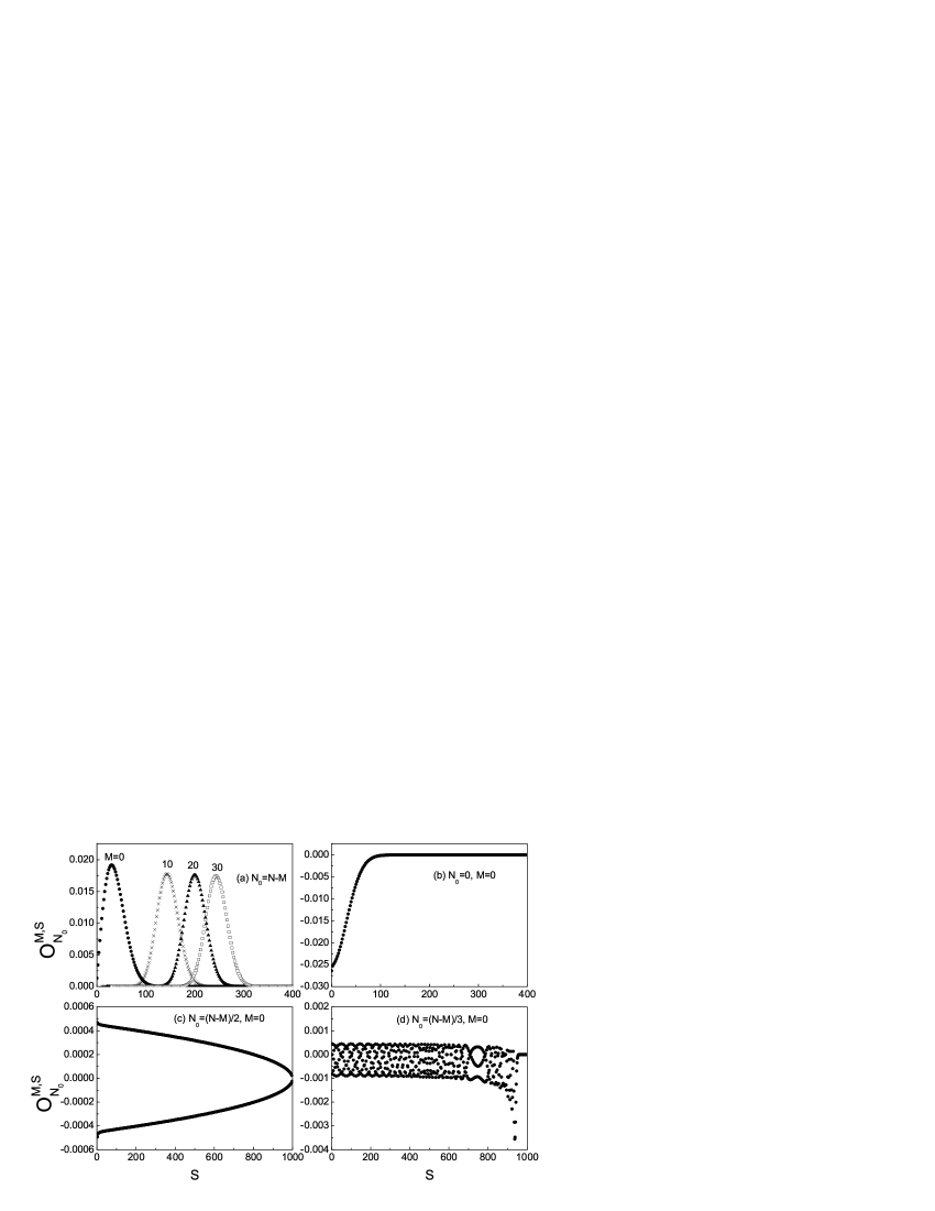
Figure 1: $O^{M,S}_{N_{0}}$ versus $S$. $N=1000$ is given (the same in the follows).

Figure 2: Evolution of the average population with $\mu=0$.

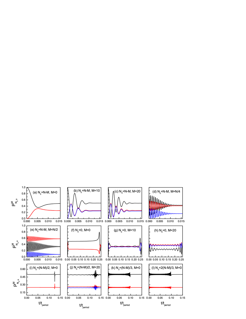
Figure 3: Evolution of the average populations with $\mu=0$ (black), $1$ (red), and $-1$ (blue). For the case $M=0$, the red and blue lines overlap.

References

(1) Tin-Lun Ho, Phys. Rev. Lett., 81, 742 (1998)
(2) D.M. Stamper-Kurn, M.R. Andrews, A.P. Chikkatur, S. Inouye, H.-J. Miesner, J.
Stenger, and W. Ketterle, Phys. Rev. Lett., 80, 2027(1998)
(3) J. Stenger, S. Inouye, D. M. Stamper-Kurn, H. -J. Miesner, A. P. Chikkatur,
and W. Ketterle, Nature (London) 396, 345 (1998).
(4) A. Goelitz, T. L. Gustavson, A. E. Leanhardt, R. Low, A. P. Chikkatur,
S. Gupta, S. Inouye, D. E. Pritchard, and W. Ketterle, Phys. Rev.
Lett., 90, 090401 (2003)
(5) A. Griesmaier, J.
Werner, S. Hensler, J. Stuhler, and T. Pfau, Phys. Rev. Lett.,
94, 160401(2005)
(6) A. Sorensen, L.-M. Duan, J.I. Cirac, and P. Zoller,
Nature 409, 63 (2001)
(7) L.-M. Duan, J.I. Cirac, and P. Zoller, Phys. Rev. A
65, 033619(2002)
(8) K. Molmer and P. Zoller, Phys. Rev. A50, 67(1994)
(9) M.-S. Chang, C.D. Hamley, M.D. Barrett, J.A.
Sauer, K.M. Fortier, W.Zhang, L. You, and M.S. Chapman, Phys. Rev.
Lett., 92, 140403(2004)
(10) M.S. Chang, Q. Qin, W.X. Zhang, L. You, and M.S.
Chapman, Nature Physics (London) 1, 111(2005)
(11) H. Schmaljohann, M. Erhard, J. Kronjager, K. Sengstock, K. Bongs,
Appl. Phys. B-Lasers and Optics 79, 1001 (2004)
(12) C.K. Law, H. Pu, and N.P. Bigelow, Phys. Rev. Lett.,
81, 5257(1998)
(13) H. Pu, C.K. Law, S. Raghavan, J.H. Eberly, and N.P.
Bigelow, Rhys. Rev. A., 60, 1463(1999)
(14) R.B. Diener and T.L. Ho, arxiv:cond-mat/0608732
(2006)
(15) C.G. Bao and Z.B. Li, Phys. Rev. A 70, 043620 (2004)
(16) C.G. Bao and Z.B. Li, Phys. Rev. A 72, 043614 (2005)
(17) C.G. Bao, Frontier in Physics in China 1, 92 (2006)
(18) Z.B. Li and C.G. Bao, preprint, cond-mat/0703737.
(19) A.R. Edmonds, Angular Momentum in Quantum Mechanics (Princeton, New Jersey, 1960)