A Study on anisotropy of cosmic ray distribution with a small array of water cherenkov detectors

Abstract

$\cos 6{\cdot 71{\cdot}4}$ The study of the anisotropy of the arrival directions is an essential tool to investigate the origin and propagation of cosmic rays primaries. A simple way of recording many cosmic rays is to record coincidences between a number of detectors. We have monitored multi-TeV cosmic rays by a small array of water cherenkov detectors in Tehran($35^{\circ}43^{\prime}$ N, $51^{\circ}20^{\prime}$E, $1200$m a.s.l). More than $1.1\times 10^{6}$ extensive air shower events were recorded. In addition to the Compton- Getting effect due to the motion of the earth in the Galaxy, an anisotropy has been observed which is due to a unidirectional anisotropy of cosmic ray flow along the Galactic arms.

I Introduction

Although Cosmic Rays( CRs) have been known for almost one century, their origin remains uncertain, mostly because their trajectories are bent by Galactic magnetic fields and they do not individually point back to their sources. Cosmic rays in the lower energy range have gyro radii of about 1pc or less in typical galactic magnetic fields( a proton with an energy of $10^{15}$eV would have a gyro radius of 1 pc in a $1\mu$G field). Moreover, since these fields are chaotic on scales ranging at least from $10^{8}$cm to $10^{20}$cm Armstrong et al. (1995), the transport of CRs is diffusive up to high energies, which tends to make their angular distribution isotropic. Therefore, even collectively, the CR arrival directions hold virtually no information about the source distribution in space. However, as the energy of the CRs increases, it acan appear either because the diffusive approximation does not hold anymore, or because the diffusion coefficient becomes large enough to reveal intrinsic inhomogeneities in the source distribution. Specifically, even if the diffusive regime holds, the density of CR sources in the Galaxy is believed to be larger in the inner regions than in the outer ones, and this can cause a slightly higher CR flux coming from the Galactic center than from the anti-center. Meanwhile, the global CR streaming away from the Galactic plane( towards the halo) can be a source of measurable anisotropy. However, the detailed angular distribution of CRs is quite hard to predict, even if we assume a definite source distribution, because it also depends on the propagation conditions, which are related to both large scale and small scale magnetic field configurations, and on the position of the Earth relative to major magnetic structures, such as the local Galactic arm.

From a general point of view, the characterization of the CR anisotropy provides useful information to constrain the GCR diffusion models, notably the effective diffusion coefficients, related to the magnetic field structure. Indeed the level of CR anisotropy depends on the diffusion coefficient, $D$: in a simple model where CR sources are homogeneously distributed in a disk of thickness $2h$ and the CRs are confined in a halo of height $H$, the anisotropy at a distance $z$ above the Galactic plane($z<h$) is estimated as $\Delta\simeq 3D/cH\times z/h$ Ptuskin (1997). The deviation from isotropy is typically below $1\%$ and can be as low as $0.03\%$ Smith & Clay (1997). Anisotropy measurements at various energies can thus provide crucial information about the energy dependence of the diffusion coefficient. This information is particularly important to constrain the GCR source spectrum, since it sets the relation between the source power law index and the observed one, through the energy dependent confinement of CRs in the Galaxy. This diffusion maybe is broadly along the magnetic field lines which are in tubes of dimensions greater than the gyro radii. So the direction of the peak of the anisotropy would indicate the direction back towards the cosmic ray source, and the amplitude of the anisotropy would give information on the scattering process involved in the diffusion. Specifically, an estimate of the mean free path might be obtained.

The anisotropy is due to a combination of effects. Compton and GettingCompton & Getting 1935 (1935) proposed in 1935 that the motion of the solar system relative to the rest frame of the cosmic ray plasma should cause an energy independent dipole anisotropy with maximum in the direction of motion. The earth’s rapid motion in space, resulting from the rotation of our galaxy, results variations in cosmic ray intensity fore and aft of the earth’s motion. Following Compton - Getting (1935), the magnitude of the anisotropy is expressed as

$$\eta=(\gamma+2)\frac{u}{c}\cos\beta,\\$$ (1)

where $\gamma$ denotes the power law index of the energy spectrum of cosmic rays, $u$ the velocity of the detector relative to the production frame of the cosmic rays ( where they are presumed to be isotropic), $c$ the speed of light, and $\beta$ the cosmic ray direction relative to $u$, i.e. $\cos\beta$ is the projection of the cosmic ray along the forward direction of $u$. In fact the value of $(\gamma+2)\frac{u}{c}$ is $(f_{max}-f_{min})/(f_{max}+f_{min})$ with $f_{max}$ the counting rate along the direction of the velocity and $f_{min}$ along the contrary direction. The magnitude of the anisotropy is extremely small and independent of the cosmic ray energy. Our data will be analyzed in a sun-centered frame, and so if data accumulation is done over an integer number of solar years, it is only necessary that the orbital speed of the Earth around the sun($\sim 30$km s^-1) be considered. The large effect due to the Galactic rotational speed (220 km s^-1) will cancel out as the data are averaged over this time Poirier et al. (2001). Many experiments have been carried out for detection of this effectPoirier et al. (2001); Lin et al. (1999).

Doppler effect studies of globular clusters and extra galactic nebulae have revealed a motion of the earth of about 220km s^-1 towards right ascension $\alpha\simeq 21$h and declination $\delta\simeq 47^{\circ}$N due chiefly to the rotation of the Galaxy. This motion, with a speed of about 0.1% $c$ will affect the intensity of the incoming cosmic rays by changing both the energy of the cosmic ray particles and the number received per second. Using value of 220 km$s^{-1}$ for $u$, and 2.7 for the spectral index, Eqn. (1) gives a Compton Getting Effect(CGE) amplitude of $0.345\times 10^{-2}$ for the fractional forward-backward asymmetry caused by the motion of the earth in the Galaxy.

Another effect that can produce sidereal modulation is solar diurnal and seasonal changes in the atmospheric temperature and pressure. As the atmospheric temperature and pressure change during the course of a day, the balance of cosmic ray secondary particle interaction and decay changes. This propagates to changes in the detection rate that depend on the detector type( air shower, underground muon, surface muon) and on the energy threshold. These changes tend to have a strong Fourier component with a frequency of one solar day($\simeq 365$ cycles/ year) and one solar year( 1 cycle/ year). In some( but by no means all) experiments, the interplay between the daily and seasonal modulation can produce significant modulation in sideband frequencies of $\simeq(365\pm 1)$cycles/ yearFarley & Storey (1954). The modulation with frequency 366 cycles/ year appears as a sidereal modulation. The size of the atmospheric contribution to apparent sidereal anisotropy can be estimated from the amplitude of the pseudo- sidereal( 365 cycles/ year) frequency. If it is large, the atmospheric effect can be subtracted using the amplitude and phase of the pseudo- sidereal component. The anisotropy that remains after accounting for the Compton- Getting and atmospheric effects is due to solar and galactic effects. At the lowest energies($\sim 100$GeV), the Interplanetary Magnetic Field( IMF) produced by the solar wind effects the sidereal anisotropy: when the local IMF points toward the sun, the anisotropy peaks at about 18hr right ascension, while it peaks at 6hr when it points awayKojima et al. (2001, 2003). The average over the two configurations produces a small, residual anisotropy peaking at around 2-4hr. At higher energies, local IMF plays a negligible role. Instead, the heliosphere extending to distances of order 100AU is believed to induce anisotropy in cosmic rays with energies around 1TeVNagashima et al. (1989, 1989). Beyond this energy, the anisotropy is believed to be primarily of galactic origin. For instance, the galactic magnetic field around the solar system neighborhood could produce anisotropy. Also, an uneven distribution of sources of cosmic rays ( presumably, mostly supernova remnants) may produce anisotropy. It is believed that star formation( and thus, supernova remnants) occur primarily in the spiral arms of the galaxy. The earth is located at the inner edge of the Orion spur. Thus, in the direction of the Orion spur( galactic longitude between $60^{\circ}$ to $270^{\circ}$) they are distributed nearby sources of cosmic rays, while in the complementary direction, they are much further away.

Because of small anisotropy, large data sets are required to make useful measurements which overcome the statistical uncertainties of counting experiments. A simple way of recording many cosmic rays is to record coincidences between a number of detectors. Few statistically significant anisotropies have been reported from extensive air shower experiments in the two last decades. Aglietta et al.( 1996,EAS-TOP)Aglietta et al. (1996) published an amplitude of $(3.7\pm 0.6)\times 10^{-4}$ and phase $\phi=(1.8\pm 0.5)$hr LST, at $E_{\circ}\approx 200$TeV. Analysing the Akeno experiment, Kifune et al.(1986)Kifune et al. (1986) reported results of about $2\times 10^{-3}$ at about 5 to 10 PeV. An overview of experimental results can be found in Clay et al. (1997).We have operated a small array of water cherenkov detectors on the roof of physics department at Sharif University of Technology in Tehran($35^{\circ}43^{\prime}$ N, $51^{\circ}20^{\prime}$E, $1200$m a.s.l=890 gcm^-2) as a prototype for constructing an Extensive Air Shower(EAS) array on Alborz mountain range at altitude of over 2500m near Tehran.

The main purpose of this article is to study the unidirectional anisotropy of cosmic rays flow along the Galactic arms which was observed in the sidereal time at energies above 50 TeV. We describe the experimental setup in section II, and the data analysis and discussion in section III.

II Experimental setup

Four Water Cherenkov Detectors( WCDs) used for recording Extensive Air Showers( EASs). The four WCDs consist of cylindrical tanks made of polyethylene with a diameter of 64cm and a height of 130cm filled up to a height of 120cm with 382 liters of purified water. All the inner surfaces of the four Cherenkov tanks were optically sealed and covered with white paint which reflects light in a diffusive way. Each one of them have a single 5.2cm PMT( model EMI 9813KB) located at the top of the water level along the cylinder axis. The array arranged in a square with side 608cm as shown in Fig.1, on the roof of the Physics Department at Sharif university of Technology in Tehran($35^{\circ}43^{\prime}$ N, $51^{\circ}20^{\prime}$E, $1200$m a.s.l=890 gcm^-2). The signal produced by secondary particles of an EAS are triggered with an amplitude threshold of -500mV by an 8-fold fast discriminator( CAEN N413A). The threshold of each discriminator is set at the separation point between the signal and background noise levels. The discriminator outputs are connected to one of three Time to Amplitude Converters( TAC) (EG&G ORTEC 566) which are set to a full scale of 200ns ( maximum acceptable time difference between two WCDs). The output of due to the No.3 WCD is connected to the start inputs of TAC1, TAC2, and TAC3. The outputs of due to No.1, 2, and 4 WCDs are respectively connected to the stop inputs of TAC1, TAC2, and TAC3. then the outputs of these three TACs are fed into a multi-parameter Multi channel Analyzer( MCA) ( KIAN AFROUZ Inc.) via an Analogue to Digital Converter ( ADC)( KIAN AFROUZ Inc.) unit. The output of TAC1 triggers the ADC, and the 3 time lags between the output signals of PMTs (3,1), (3,2), and (3,4) are read out as parameters 1 to 3. So by this procedure an event is logged.

III Data Analysis and Discussion

III.1 Array event rate

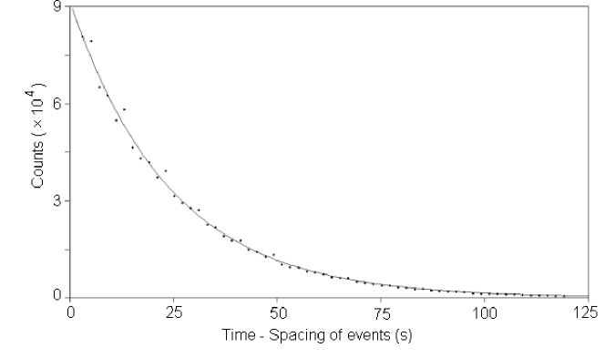
Figure 2: Distribution of events time-spacing.

The data set covers a total period of $2.7\times 10^{7}$ seconds. A total of $1.1\times 10^{6}$ events with zenith angles $\leq 60^{\circ}$ were collected during this time, giving a mean event rate of one event every 24.5 seconds. Figure 2 shows the events time- spacing distribution. Since events arrive randomly in time, it is expected that this will follow an exponential distribution, $viz.$

$$f(t)=f(0)\exp(-t/\tau).\\$$ (2)

The event rate can be obtained by fitting this function on the events time-spacing distribution. One event per every $\tau=24.1$s is obtained from the fit. A non-random component for the cosmic ray flux for example a point source of gamma ray gives rise to deviation from the exponential law. Our observed distribution is in good agreement with the exponential law.

III.2 Atmospheric effects on counting rate

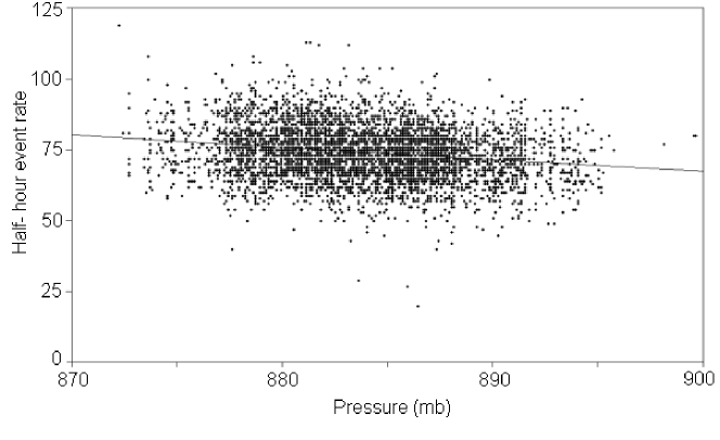
Figure 3: Event rates per half an hour as a function of atmospheric pressure.

The rate of shower detections depends on a number of factors. If either temperature or pressure variations have Fourier components in solar or sidereal times, spurious components may be introduced into the shower detection rate Farley & Storey (1954). Various methods are used in order to study the dependence of event rate on atmospheric ground pressure, $p$, and temperature, $T$, Antoni et al. (2004). In a multiple regression analysis of event rate against pressure and temperature, the temperature effect is found to be statistically insignificant. The CR intensity dependence on barometric pressures in half-hour intervals are shown in Fig. 3. We can describe the dependence by the following function

$$R=R_{0}\exp(\frac{p_{0}-p_{i}}{p_{1}})\\$$ (3)

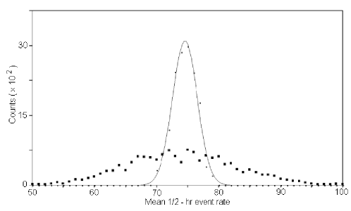
Figure 4: Distribution of mean 1/2-hr event rates before (squares) and after (points) the atmospheric correction for pressure. The line curve shows a fit by a Gaussian function.

The values of $R_{0}=74$ events per half an hour, $p_{0}$=883.7mb, and $p_{1}$=171.5mb were obtained from the data. $p_{i}$ denotes the measured air pressure at a given time. By this empirical function, we weighted the raw event rates for atmospheric pressure. Figure 4 shows the mean half-hour event rate distributions with and without correction for atmospheric ground pressure. The distribution of corrected rates is consistent with a Gaussian distribution, as expected for the statistical fluctuation of the events rate, and there is no residual temperature effect.

III.3 Zenithal angle distribution of the EAS events

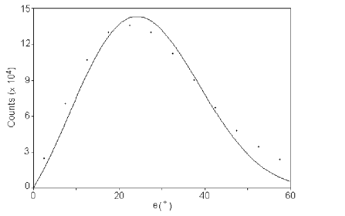
Figure 5: Frequency of air showers vs. zenith angle.

Since the thickness of the atmosphere increases with increasing zenith angle, $\theta$, the number of EAS events is strongly related to $\theta$, as shown in Fig. 5. The differential zenith angle distribution can be represented by

$$dN=constant.(\delta_{1}\cos\theta+\delta_{2}\sin\theta)\cos^{n}\theta\sin\theta d\theta.\\$$ (4)

Where we split into particles entering through the lid of cylinderical tank of WCD or through its walls. The first term in parenthesis of Eqn.(4) is related to the lid and the second to the walls. The parameter $\delta_{1}$ includes the area of lid surface, $S_{1}$, and detection probability of particles entering through the lid, $P_{1}$. The parameter $\delta_{2}$ also includes the greatest surface area of vertical profile of the WCD, $S_{2}$, and detection probability of particles entering through its walls, $P_{2}$. So we can split $\delta_{j}(j=1,2)$ in the form of

$$\delta_{j}=S_{j}P_{j},$$ (5)

where only $P_{j}$s are determined from the simulation ( see the Appendix). $S_{1}$ and $S_{2}$ are respectively $3.2\times 10^{3}$cm² and $7.68\times 10^{3}$cm². By fitting Eqn (4) on our experimental data, $n=7.3$ is obtained.

III.4 Energy Threshold of our experiment

Since we can not determine the energy of the showers on an event-by-event basis, we estimate the energy threshold of our array by the CORSIKA code for simulation of EAS events Heck et al. (1998). In order to record a shower it is necessary at least one particle passes through each of the four WCDs. Because our array has been arranged in a square with side 608cm we can detect a shower if density of secondary particles to be at least $\rho_{r}=1/S_{eff}$ particles cm^-2 at $r=608\times\sqrt{2}/2=420$cm, where $S_{eff}$ is the effective surface area of a WCD. This area is calculated as follows:

$$S_{eff}=\frac{\int_{0}^{\pi/3}(P_{1}S_{1}\cos\theta+P_{2}S_{2}\sin\theta)\sin\theta d\theta}{\int_{0}^{\pi/3}\sin\theta d\theta}=6.5\times 10^{3}~{}{\rm cm}^{2},$$ (6)

with $P_{1}=0.88$, $S_{1}=3.2\times 10^{3}$cm², $P_{2}=0.93$, and $S_{2}=7.68\times 10^{3}$cm². The upper limit, $\pi/3$, is due to events selection with zenith angles $\leq\pi/3$. We simulated more than $10^{5}$ EAS events with CORSIKA code using the hadronic interaction models QGSJET and GHEISHA. The energy range for primary particles was selected from 5TeV to 5PeV, with differential flux given by $dN/dE\propto E^{-2.7}$ . These simulations are in different directions with zenith angle from $0^{\circ}$ to $60^{\circ}$ and azimuth angle from $0^{\circ}$ to $360^{\circ}$. Finally from the CORSIKA simulations with $\rho_{r}=1.5\times 10^{-4}$particles cm^-2 at $r=420$cm, we obtained the energy threshold $E_{th}=50$TeV.

III.5 Sidereal time distribution

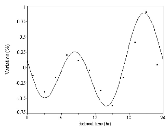
Figure 6: Observed sidereal time variation in intensity of the cosmic rays (points). The curve is the best fit to Eqn. (7) with the coefficients as listed in Table I.

After atmospheric correction we calculated the sidereal time (ST) from $ST=ST_{\circ}+\alpha(ZT-ZT_{0}$). $ST_{0}$ can be looked up in an almanac for the time $ZT_{0}$, $ZT$ is the solar time, and $\alpha=1.00273790935$. Figure 6 shows percentage variation in intensity of the cosmic rays with sidereal time. The data have been fit to Eqn.(7) which describes a curve with first and second harmonics( i.e with a once-per-day and a twice-per-day variation),

$$y=A_{I}\cos[\frac{2\pi}{24}(t-T_{I})]+A_{II}\cos[\frac{2\pi}{12}(t-T_{II})].$$ (7)

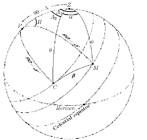
Figure 7: Celestial coordinate, C= direction of cosmic ray, M= direction of earth’s motion, Z= zenith, P= direction of North pole.

Where t is in hours. The fitting results of data are summarized in Table I. The CGE would contribute to the component $A_{I}$ in the sidereal time asymmetry. This analysis shows that the anisotropy has a peak close to the sidereal time 21h, when the zenith is toward the earth’s motion. The amplitude of the first harmonic is $0.32\%$. So there is a definite sidereal time variation whose phase and amplitude are close to those predicted. In order to calculate the magnitude of anisotropy due to CGE i.e the value $\eta$ in Eqn.(1), a mean value for $\cos\beta$ is needed. Assume $\delta$ is the declination of the direction of earth’s motion, $\lambda$ the latitude of the observer and $H$ the hour angle between the observer’s meridian and the direction of motion, then to consider Fig.7 the angle $\phi$ between the observer’s zenith and the direction of earth’s motion is given by

$$\cos\phi=\sin\delta\sin\lambda+\cos\delta\cos\lambda\cos H.$$ (8)

On the other hand, $\cos\beta$ is calculated by

$$\cos\beta=\cos\phi\cos\theta+\sin\phi\sin\theta\cos\alpha.$$ (9)

Where $\theta$ is the zenith angle of cosmic ray and $\alpha$ difference between the azimuth angle of the direction of motion and of cosmic ray( Fig.7), that is $\alpha=A_{1}-A_{2}$, which $A_{1}$ and $A_{2}$ are obtained by

$$\sin\delta=\sin\lambda\cos\phi+\cos\lambda\sin\phi\cos A_{1},$$ (10)

and

$$\sin\delta^{\prime}=\sin\lambda\cos\theta+\cos\lambda\sin\theta\cos A_{2}.$$ (11)

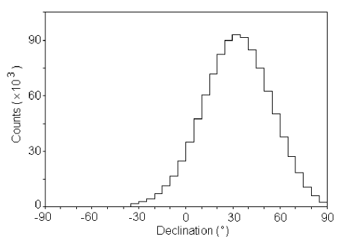
Figure 8: Distribution of air shower events vs. declination angle.

Where $\delta^{\prime}$ is the declination of cosmic ray. According to Eqns (8) to (11), the 24-hour mean of the component of cosmic ray in the direction of motion ($\cos\beta$) may be obtained. Using $\lambda=35^{\circ}43^{{}^{\prime}}$ and $\delta=47^{\circ}$, we calculated the 24-hour mean value of $\cos\phi\simeq 0.43$ with Eqn.(8). With distribution of $(P_{1}S_{1}\cos\theta+P_{2}S_{2}\sin\theta)\cos^{7.3}\theta\sin\theta$ which describes the acceptance of detectors and the cosmic ray absorption in the Earth’s atmosphere because of inclination from the vertical direction in Tehran ( section III, C) we calculated the mean value of $\cos\theta$=0.88. Also the mean values of $A_{1}$ and $A_{2}$ were obtained by using the mean value $\delta^{\prime}$. Figure 8 shows the distribution of cosmic rays declination. The mean value of declination is $\delta^{\prime}=32.5^{\circ}$. From Eqns. (10) and (11), $A_{1}$ and $A_{2}$ obtain $49^{\circ}$ and $86^{\circ}$ respectively. Finally from Eqn.(9) a value of 0.72 is obtained for $\cos\beta$ and this is multiplied by the expected CGE amplitude of $0.345\%$ to yield a predicted effect of expected value of 0.248%. The value obtained from experimental data is $0.32\%$ which about $0.07\%$ is more than the CGE value. This remaining asymmetry of $0.07\%$, presumably has an origin different to the that of the CGE.

Since the recorded data are in Tehran with latitude $35^{\circ}43^{\prime}N$, the majority of cosmic rays are from the spiral arm inwards direction, which is at about 20h in right ascension and $35^{\circ}$ in declinationJacklyn (1986). So the remaining asymmetry is probably due to unidirectional anisotropy of cosmic ray flow along the Galactic arms. A simple diffusion model Allan (1972) suggests that value of this asymmetry, $0.07\%$, would be roughly equal to the ratio of the scattering mean free path to a characteristic dimension of the containment region ( i.e the central Galactic region, with a scale of 10kpc). So with amplitude of the anisotropy of $0.07\%$ found in this work, we obtain a mean free path of about 7pc which is about perhaps 7 gyro radii.

Since the anisotropies are low, it is necessary to consider the effect of counting statistics for a finite measured data set. If we have N events then the probability of getting a fractional amplitude greater than $r$ is given by Linsley (1975),

$$P(>r)=e^{-k_{0}},k_{0}=r^{2}N/4.$$ (12)

So a convenient parameter for characterizing the anisotropy amplitude probability distribution is $k_{0}$. We can take $\sqrt{2}r_{rms}$ which corresponds to $k_{0}$ =1, as noise amplitude. For the number of events that we have accumulated, $1.1\times 10^{6}$, the total amplitude of $0.32\%$ obtained in this work can be arisen by chance with a probability of $\sim 0.06$ corresponding to $k_{0}=2.8$. This shows a significant anisotropy( $k_{0}>1$) at the sidereal period. So we conclude that this data set gives evidence of anisotropy.

IV Conclusion

Cosmic ray data in Alborz observatory clearly shows an anisotropy in sidereal time with the energy threshold of $\sim 50$TeV and the mean energy of $\sim 121$TeV. One part of this anisotropy is due to Earth’s motion around the Galaxy (the CGE), but our measured asymmetry suggests the possible existence of some other additional effects, probably a unidirectional anisotropy of cosmic ray flow along the Galactic arms. The first harmonic amplitude of our total measured anisotropy is about $0.32\%$. The CGE contribution to this anisotropy is about $0.248\%$ and the rest, $0.07\%$, is predicted to be due to the flow along the Galactic arm. The latter anisotropy suggests a mean free path of about 7pc for these high-energy cosmic rays. The evidence of these anisotropies is based on the value of the parameter $k_{0}$, as suggested by Linsley( 1975) and found in this work to be 2.8, that is, more than $k_{0}=1$, the value for the noise amplitude.

The EAS-TOP experiment reported somewhat lower limits in the energy range below 1200TeVAglietta et al. (2003). The relatively large amplitudes published by the Akeno experimentKifune et al. (1986) and our experiment are difficult to reconcile with the results of the EAS-TOP experiment.

Appendix

In order to obtain the $P_{j}$s, Eqn.(5), we first calculated the track length of particle passing through lid and walls of WCD. To determine the track length distribution we have made the following assumption:

A) The zenithal and azimuth angles of particles are uniformly distributed.

B) The random distribution increases linearly with $r$, the distance from center of lid, i.e. it is proportional to the annulus surface $2\pi r\Delta r$.

The geometry can be simply solved. It is split into particles entering through the lid or through the walls as seen in Fig. 1. In these figures, $r$ is the distance from the center of the cylinder, the tank radius is $R_{0}=32$cm, the tank height $H_{0}=120$cm, and $\varphi$ and $\theta$ are azimuth and zenith angles of particle, respectively. The simulation process starts by randomly choosing $r$ which increases linearly with $r$. Then $\varphi$ and $\theta$ are randomly chosen and the track lengths within the tank are evaluated by a simple calculation ( the particle could either leave through the wall or the bottom lid, as shown in Fig. 1).

Then the number of photons produced along a flight path was estimated. Charged particles emit light under a characteristic angle when passing through a medium if their velocity exceeds the speed of light in the medium. The Cherenkov angle is related to the particle velocity and the refractive index of the medium $n$( $\cos\theta=1/n\beta$). For relativistic particles, $\beta=1$, and the refractive index of purified water, $n=1.33$( for short wavelengths of visible region), the Cherenkov light is emitted under $41^{\circ}$. The number of photons produced along a flight path $dx$ in a wave length bin $d\lambda$ for a particle carrying unit charge is :

$$\frac{d^{2}N}{dxd\lambda}=\frac{2\pi\alpha\sin^{2}\theta}{\lambda^{2}},$$ (13)

where $\alpha=1/137$. At wavelengths of 310-470nm the efficiency of the photomultiplier is maximal. Within 1cm flight path 220 photons are emitted in this wavelength bin. To consider the effective area of the photomultiplier( 21.2cm²), and neglecting absorption and scattering effects in water we obtained the number of photons received by PMT ( Fig. 9). Finally with a $\eta=25\%$ quantum efficiency and a G=$10^{8}$ gain for the PMT, the number of electrons produced in PMT($N_{e}=N_{photon}\eta G$) was calculated. As we know, the output signal at the PMT’s anode is a current or charge pulse. Now to consider the amplitude threshold of discriminator ( -500mV), and the anode load resistor and capacitance, we obtained that for producing a pulse with amplitude -500mV, the number of photons received to PMT should be more than 1. Because the quantum efficiency of PMT is 25% using Fig. 9 we calculated the detection probability, $P_{j}$s, are respectively 0.88 and 0.93 for lid and walls WCD.

Amplitude(%)	Phase(h)
$A_{I}=0.32\pm 0.10$	$T_{I}=21.3\pm 1.0$
$A_{II}=0.56\pm 0.10$	$T_{II}=20.6\pm 0.7$

Table 1: Parameters of the fit coefficients in equation(7)

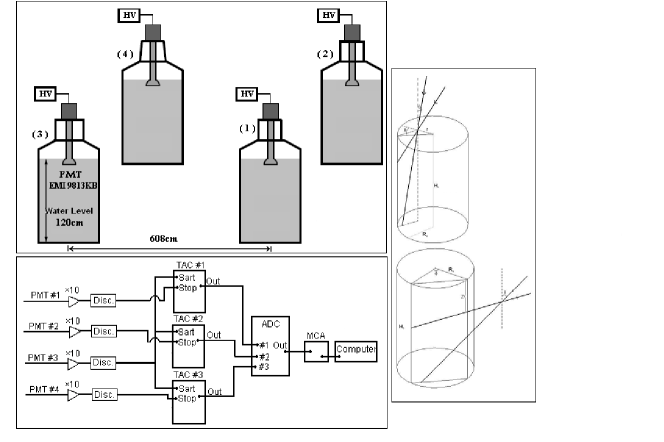
Figure 1: Schematic view of water Cherenkov detectors as a square array, and the electronic circuit. Particle tracks through lid (right hand-top), and tracks through walls( right hand-bottom) have also been shown.

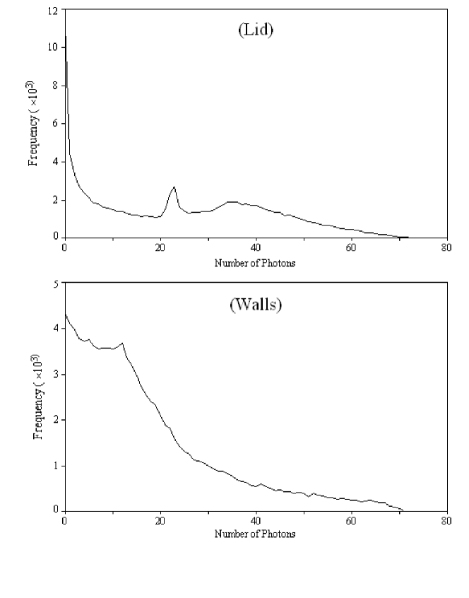
Figure 9: The number of photons received by PMT in consequence of particle passing along different tracks entering through the lid( Top), and the walls( bottom).

References

- Armstrong et al. (1995) J.W. Armstrong, B.J. Rickett, and S.R. Spangler, ApJ 443, 209 (1995)
- Ptuskin (1997) V. S. Ptuskin, Adv. Space Res. 19, 697 (1997)
- Smith & Clay (1997) A.G.K. Smith and R.W. Clay, Aust. J. Phys. 50, 827 (1997)
- Compton & Getting 1935 (1935) A.H. Compton, and I.A. Getting, Phys. Rev. 47, 817 (1935)
- Poirier et al. (2001) J. Poirier, and C. D’Andrea, M. Dunford, Proc. 27th ICRC, Hamburg, Germany , 3930 (2001)
- Lin et al. (1999) T.F. Lin et al., Proc. 26th ICRC, Salt Lake city, USA , HE2.2.09, 100 (1999)
- Farley & Storey (1954) F. J. M Farley, and J. R. Storey, Proc. phys. Soc. , 996 (1954)
- Kojima et al. (2001) H. Kojima et al., Proc. 27th ICRC, Hamburg, Germany , 3943 (2001)
- Kojima et al. (2003) H. Kojima et al., Proc. 28th ICRC, Tsukuba, Japan , 3957 (2003)
- Nagashima et al. (1989) K. Nagashima et al., Nuovo Cimento Soc. Ital. Fis. , 695 (1989)
- Nagashima et al. (1989) K. Nagashima et al., K. Fujimoto, and R.M. Jacklyn, J. Geophys. Res. , 17429 (1998)
- Aglietta et al. (1996) M. Aglietta et al., APJ , 501 (1996)
- Kifune et al. (1986) T. Kifune et al., J. Phys. G , 129 (1986)
- Clay et al. (1997) R. Clay et al., Proc. of 25th ICRC, Durban , 185 (1997)
- Antoni et al. (2004) T. Antoni et al., ApJ , 687 (2004)
- Heck et al. (1998) D. Heck et al., Report FZKA6019 (Forschungszentrum Karlsruhe) , (1998) .
- (17) tycho.usno.navy.mil/sidereal.html
- Jacklyn (1986) R.M. Jacklyn, PASA , 425 (1986)
- Allan (1972) H.R. Allan, ApJ. Lett. , 237 (1986)
- Linsley (1975) J. Linsley, Phys. Rev. Letts. , 1530 (1975)
- Aglietta et al. (2003) M. Aglietta et al., Proc. of 28th ICRC, Tsukuba, Japan , 183 (2003)