Optimizing Scrip Systems: Efficiency, Crashes, Hoarders, and Altruists

Abstract

We discuss the design of efficient scrip systems and develop tools for empirically analyzing them. For those interested in the empirical study of scrip systems,

we demonstrate how characteristics of agents in a system can be inferred from the equilibrium distribution of money. From the perspective of a system designer, we examine the effect of the money supply on social welfare and show that social welfare is maximized by increasing the money supply up to the point that the system experiences a “monetary crash,” where money is sufficiently devalued that no agent is willing to perform a service. We also examine the implications of the presence of altruists and hoarders on the performance of the system. While a small number of altruists may improve social welfare, too many can also cause the system to experience a monetary crash, which may be bad for social welfare. Hoarders generally decrease social welfare but, surprisingly, they also promote system stability by helping prevent monetary crashes. In addition, we provide new technical tools for analyzing and computing equilibria by showing that our model exhibits strategic complementarities, which implies that there exist equilibria in pure strategies that can be computed efficiently.

1 Introduction

Historically, non-governmental organizations have issued their own currencies for a wide variety of purposes. These currencies, known as scrip, have been used in company towns where government issued

currency was scarce [18], in Washington DC to reduce the robbery rate of bus drivers [21], and in Ithaca (New York) to promote fairer pay and improve the local economy [8]. Scrip systems are also becoming more prevalent in online systems. To give just some examples, the currencies of online virtual worlds such as Everquest and Second Life are a form of scrip; market-based solutions using scrip systems have been suggested

for applications such as system-resource allocation [12], managing replication and query

optimization in a distributed database [15], and allocating experimental time on a wireless sensor network test bed [3]; a number of sophisticated scrip systems have been proposed [5, 7, 20] to allow agents to pool resources while avoiding what is known as free riding, where agents take advantage of the resources the system provides while providing none of their own (as Adar and Huberman 2 have shown, this behavior certainly takes place in systems such as Gnutella); and Yootles 14 uses a scrip system as a way of helping groups make decisions using economic mechanisms without involving real money.

Creating a scrip system creates a new market where goods and services can be exchanged that may have been impractical or undesirable to implement with standard currency. However, the potential benefits of a scrip system will not necessarily be realized simply by creating the framework to support one. The story of the Capitol Hill Baby Sitting Co-op 16, popularized by Krugman 10, provides a cautionary tale. The Capitol Hill Baby Sitting Co-op was a group of parents working on Capitol Hill who agreed to cooperate to provide babysitting services to each other. In order to enforce fairness, they issued a supply of scrip with each coupon worth a half hour of babysitting. At one point, the co-op had a recession. Many people wanted to save up coupons for when they wanted to spend an evening out. As a result, they went out less and looked for more opportunities to babysit. Since a couple could earn coupons only when another couple went out, no one could accumulate more, and the problem only got worse.

After a number of failed attempts to solve the problem, such as mandating a certain frequency of going out, the co-op started issuing more coupons. The results were striking. Since couples had a sufficient reserve of coupons, they were more comfortable spending them. This in turn made it much easier to earn coupons when a couple’s supply got low. Unfortunately, the amount of scrip grew to the point that most of the couples felt “rich.” They had enough scrip for the foreseeable future, so naturally they didn’t want to devote their evening to babysitting. As a result, couples who wanted to go out were unable to find another couple willing to babysit.

This anecdote shows that the amount of scrip in circulation can have a significant impact on the effectiveness of a scrip system. If there is too little money in the system, few agents will be able to afford service. At the other extreme, if there is too much money in the system, people feel rich and stop looking for work. Both of these extremes lead to inefficient outcomes. This suggests that there is an optimal amount of money, and that nontrivial deviations from the optimum towards either extreme can lead to significant degradation in the performance of the system.

Motivated by these observations, we study the behavior of scrip systems with a heterogeneous population of agents. We prove a number of theoretical

results, and use them to gain insights into the design and analysis of practical scrip systems.

The motivation for our interest in heterogeneous populations of agents should be clear. In the babysitting coop example, we would not expect all couples to feel equally strongly about going out nor to feel the “pain” of babysitting equally. In earlier work 4, we showed that with a homogeneous population of agents, we could assume that all agents were following a threshold strategy: an agent who has more than a certain threshold of money will not volunteer to work; below the threshold, he will volunteer. Perhaps not surprisingly, we show that even with a heterogeneous population, each different type of agent can still be characterized by a threshold (although different types of agents will have different thresholds).

We also characterize the distribution of money in the system in equilibrium, as a function of the fraction of agents of each type. Using this characterization, we show that we can infer the threshold strategies that different types of agents are using simply from the distribution of money. This shows that, by simply observing a scrip system in operation, we can learn a great deal about the agents in the system. Not only is such information of interest to social scientists and marketers, it is also important to a system designer trying to optimize the performance of the system. This is because agents that have no money will be unable to pay for service; agents that are at their threshold are unwilling to serve others. We show that, typically, it is the number of agents with no money that has the more significant impact on the overall efficiency of the system. Thus, the way to optimize the performance of the system is to try to minimize the number of agents with no money.

As we show, we can decrease the number of agents with no money by increasing the money supply. However, this only works up to a point. Once a certain amount of money is reached, the system experiences a monetary crash: there is so much money that, in equilibrium, everyone will feel rich and no agents are willing to work. The point where the system crashes gives us a sharp threshold. We show that, to get optimal performance, we want the total amount of money in the system to be as close as possible to the threshold, but not to go over it. If the amount of money in the system is over threshold, we get the worst possible equilibrium, where all agents have utility 0.

The analysis above assumes that all users have somewhat similar motivation: in particular, they do not get pleasure simply from performing a service, and are interested in money only to the extent that they can use it to get services performed. But in real systems, not all agents have this motivation. Some of the more common “nonstandard” agents are altruists and hoarders. Altruists are willing to satisfy all requests, and do not require money in return; hoarders never make requests, and just hoard the money they make by satisfying requests. Studies of the Gnutella peer-to-peer file-sharing network have shown that one percent of agents satisfy fifty percent of the requests 2. These agents are doing significantly more work for others than they will ever have done for them, so can be viewed as altruists. Anecdotal evidence also suggests that the introduction of any sort of currency seems to inspire hoarding behavior on the part of some agents, regardless of the benefit of possessing money.

Altruists and hoarders have opposite effects on a system: having altruists is essentially equivalent to adding money; having hoarders is essentially equivalent to removing it. With enough altruists in the system, the system has a monetary crash, in the sense that standard agents stop being willing to provide service, just as when there is too much money in the system. We show that, until we get to the point where the system crashes, the utility of standard agents is improved by the presence of altruists. However, they can be worse off in a system that experiences a monetary crash due to the presence of many altruists than they would be if there were no altruists at all. Similarly, we show that, as the fraction of hoarders increases, standard agents begin to suffer because there is effectively less money in circulation. On the other hand, hoarders can improve the stability of a system. Since hoarders are willing to accept an infinite amount of money, they can prevent the monetary crash that would otherwise occur as money was added. In any case, our results show that the presence of both altruists and hoarders can be mitigated by appropriately controlling the money supply.

In order to examine these issues, we use a model of a scrip system that we developed in previous work 4. While the model was developed with the workings of a peer-to-peer network in mind and assumed that all agents were identical, the model applies to a wide variety of scrip systems, and makes perfect sense even with a heterogeneous population of agents. We showed that, under reasonable assumptions, a system with only one type of agent has a cooperative equilibrium using threshold strategies. Here we extend the theoretical results to the case of multiple types of agents. We also introduce a new argument for the existence of equilibria that relies on the monotonicity of the best-reply function. We show that if some agents change their strategy to one with a higher threshold, no other agent can do better by lowering his threshold.

This makes our game one with what Milgrom and Roberts 11 call strategic complementarities,

who (using the results of Tarski 17 and Topkis 19) showed that there are pure strategy equilibria in

such games, since the process of starting with a strategy profile where everyone always volunteers (i.e., the threshold is $\infty$) and then iteratively computing the best-reply profile to it

converges to a Nash equilibrium in pure strategies. (Our earlier results guaranteed only an equilibrium in mixed strategies.) This procedure also provides an efficient algorithm for explicitly computing equilibria.

The rest of the paper is organized as follows. In Section 2, we review our earlier model. In Section 3, we prove basic results about the existence and form of equilibria. Sections 4, 5, and 6 examine the practical implications of our theoretical results. Section 4 examines the distribution of money in the system. We give an explicit formula for the distribution of money in the system based, and show how it can be used to infer the number of types of agents present and the strategy each type is using. In Section 5, we examine how a system designer can optimize the performance of the system by adjusting the money supply appropriately. Section 6 examines how altruists and hoarders affect the system. We conclude in Section 7.

2 Our Model

We begin by reviewing our earlier model of a scrip system with $n$ agents. In the system, one agent can request a service which another agent can volunteer to fulfill. When a service is performed by agent $i$ for agent $j$, agent $i$ derives some utility from having that service performed, while agent $j$ loses some utility for performing it. The amount of utility gained by having a service performed and the amount lost be performing it may depend on the agent. We assume that agents have a type $t$ drawn from some finite set $T$ of types.

We can describe the entire population of agents using the triple $(T,\vec{f},n)$, where $f_{t}$ is the fraction with type $t$ and $n$ is the total number of agents. For most of the paper, we consider only what we call standard agents. These are agents who derive no pleasure from performing a service, and for whom money has no intrinsic value. We can characterize the type of an agent by a tuple $t=(\alpha_{t},\beta_{t},\gamma_{t},\delta_{t},\rho_{t})$, where

• $\alpha_{t}$ reflects the cost of satisfying the request;

• $\beta_{t}$ is the probability that the agent can satisfy the request (an agent may not be able to satisfy all requests; for example, in a

  babysitting co-op, an agent may not be able to babysit every night);

• $\gamma_{t}$ measures the utility an agent gains for having a request satisfied;

• $\delta_{t}$ is the rate at which the agents discounts utility (so a unit of utility in $k$ steps is worth only $\delta^{k}$ as much as a unit of utility now)—intuitively, $\delta_{t}$ is a measure of an agent’s patience (the larger $\delta_{t}$ the more patient an agent is, since a unit of utility tomorrow is worth almost as much as a unit today); and

• $\rho_{t}$ represents the (relative) request rate (since not all agents make requests at the same rate) —intuitively, $\rho_{t}$ characterizes an agent’s “neediness”.

We model the system as running for an infinite number of rounds. In each round, an agent is picked with probability proportional to $\rho$ to request service. Receiving service costs some amount of scrip that we normalize to $1.

If the chosen agent does not have enough scrip, nothing will happen in this round. Otherwise, each agent of type $t$ is able to satisfy this request with probability $\beta_{t}$, independent of previous behavior. If at least one agent is able and willing to satisfy the request, and the requester has type $t$, then the requester gets a benefit of $\gamma_{t}$ utils (the job is done) and one of the volunteers is chosen at random to fulfill the request. If the chosen volunteer has type $t^{\prime}$, then that agent pays a cost of $\alpha_{t^{\prime}}$ utils, and receives a dollar as payment. The utility of all other agents is unchanged in that round. The total utility of an agent is the discounted sum of round utilities. To model the fact that requests will happen more frequently the more agents there are, we assume that the time between rounds is $1/n$.

This captures the intuition that things are really happening in parallel and that adding more agents should not change an agent’s request rate.

One significant assumption we have made here is that prices are fixed. While there are many systems with standard “posted” prices (the babysitting co-op is but one of many examples), it certainly does not always hold in practice. However, given the potential costs of negotiating prices in a large system,

it does not seem so unreasonable to assume fixed prices. Fixed prices have the added advantage of making the analysis of agent strategies simpler, because the an agent knows the future cost of

requests rather than it being set as part of the equilibrium and

potentially varying over time. We discuss this issue further at the end of Section 5.

For more discussion of this model

and its assumptions, see 4.

Our framework allows agents to differ in a number of parameters. Differences in the parameters $\alpha$, $\gamma$, and $\delta$ seem easier to deal with than differences in the other parameters because they do not affect the action of the system except through determining the optimal strategy. We refer to a population of types that differs only in these parameters as one that exhibits only payoff heterogeneity. Most of our results consider only payoff heterogeneity. We do not believe that variation $\beta$ or $\rho$ fundamentally changes our results; however, our existing techniques are insufficient to analyze this case. There is a long history of work in the economics literature on the distribution of wealth dating back to the late 19th century 13,

although this work does not consider the distribution of money in the particular setting of interest to us.

Hens et al. 6 consider a related model. There are a number of differences between the models. First, in the Hens et al. model, there is essentially only one type of agent, but an agent’s utility for providing service (our $\gamma_{t}$) may change over time. Thus, at any time, there will be agents who differ in their utility. At each round, we assume that one agent is chosen (by nature) to make a request for service, while other agents decide whether or not to provide it. In the Hens et al. model, at each round, each agent decides whether to provide service, request service, or opt out, as a function of his utilities and the amount of money he has. They assume that there is no cost for providing service and everyone is able to provide service (i.e., in our language, $\alpha_{t}=0$ and $\beta_{t}=1$). Under this assumption, a system with optimal performance is one where half the agents request service and the other half are willing to provide it.

Despite these differences, Hens et al. also show that agents will use a threshold strategy. However, although they have inefficient equilibria, because there is no cost for providing service, their model does not exhibit the monetary crashes that our model can exhibit.

3 Theoretical Results

In this section, we derive several basic results that provide insight into the behavior of scrip systems with a heterogeneous population of agents. We first show that we can focus on a particularly simple class of strategies: threshold strategies.

The strategy $S_{k}$ is the one in which the agent volunteers if and only if his current amount of money is less than some fixed threshold $k$. The intuition behind using a threshold strategy is easy to explain: A rational agent with too little money will be concerned that he will run out and then want to make a request; on the other hand, a rational agent with plenty of money would not want to work, because by the time he has managed to spend all his money, the util will have less value than the present cost of working. By choosing an appropriate threshold, a rational agent can deal with both concerns.

In 4, we showed that if there is only one type of agent, it suffices to consider only threshold strategies: we show that (under certain mild assumptions) there exists a nontrivial equilibrium where all agents use the same threshold strategy. Here, we extend this result to the case of payoff-heterogeneous agents. To prove this result, we extend the characterization of the distribution of money in a system where each agent uses the threshold strategy

provided in Theorem 3.1 of 4. To understand the characterization, note that as agents spend and earn money, the distribution of money in the system will change over time. However, some distributions will be far more likely than others. For example, consider a system with only two dollars. With $n$ agents, there are $O(n^{2})$ ways to assign the dollars to different agents and $O(n)$ ways to assign them to the same agent. If each way of assigning the two dollars to agents is equally likely, we are far more likely to see a distribution of money where two agents have one dollar each than one where a single agent has two dollars. It is well known 9 that the distribution which has the most ways of being realized is the one that maximizes entropy. (Recall that the entropy of a probability distribution on a finite space $S$ is $-\sum_{s\in S}\mu(s)\log(\mu(s))$.)

Note that many distributions have no way of being realized. For example if the average amount of money available per agent is $2 (so that if there are $n$ agents, there is $\$2n$ in the system), then the distribution where every agent has 3 dollars is impossible. Similarly, if every agent is playing $S_{3}$, then

a distribution that has some fraction of agents with $4 is impossible. Consider a scrip system where a fraction $\pi_{k}$ use strategy $S_{k}$. (We are mainly interested in cases where $\pi_{k}=0$ for all but finitely many $k$’s, but our results apply even if countably many different threshold strategies are used.) Let $M^{k}_{i}$ be the fraction of agents that play $S_{k}$ and have $i$ dollars. Then the system must satisfy the following

two constraints:

$$\sum_{k=0}^{\infty}\sum_{i=0}^{k}iM^{k}_{i} = m$$ (1)

$$\sum_{i=0}^{k}M^{k}_{i} = \pi_{k}\mbox{ for each $k$.}$$ (2)

These constraints capture the requirements that (1) the average amount of money is $m$ and (2) a fraction $\pi_{k}$ of the agents play $S_{k}$. As the following theorem shows, in equilibrium, a large system is unlikely to have a distribution far from the one that maximizes entropy subject to these constraints.

Theorem 3.1

Given a payoff-heterogeneous system with $n$ agents where a fraction $\pi_{k}$ of agents plays strategy $S_{k}$ and the average amount of money is $m$, let $M_{\vec{\pi},n,m}(t)$ be the

the random variable that gives the distribution of money in the system at time $t$, and let $M^{*}_{\vec{\pi},m}$ be the distribution that maximizes entropy subject to constraints (1) and (2). Then for all $\epsilon$, there exists $n_{\epsilon}$ such that, for all $n>n_{\epsilon}$, there exists a time $t^{*}$ such that for all $t>t^{*}$,

$$\Pr(||M_{\vec{\pi},n,m}(t)-M^{*}_{\vec{\pi},m}||_{2}>\epsilon)<\epsilon.$$

Proof 3.2.

(Sketch) This theorem is proved for the homogenous case as Theorem 3.1 of 4. Most of the proof applies without change to a payoff-heterogeneous population, but one key piece differs. This piece involves showing that each possible assignment of money to agents is equally likely; this makes maximum entropy an accurate description of the likelihood of getting a particular distribution of money. We

now prove this by considering the Markov chain whose states are the possible assignments of dollars to agents and whose transitions correspond to the possible outcomes of a round, and showing that it has a uniform limit distribution.

Proof 3.3.

A sufficient condition for the limit distribution to be uniform is that for every pair of states $s$ and $s^{\prime}$, $P_{ss^{\prime}}=P_{s^{\prime}s}$ (where

$P_{ss^{\prime}}$ is the probability of transitioning from $s$ to $s^{\prime}$).

If $P_{ss^{\prime}}>0$, there must be some pair of agents $u$ and $v$ such that

$u$ has one more dollar in state $s$ than he does in $s^{\prime}$, while $v$ has one more dollar in $s^{\prime}$ than in $s$. Every other agent must have the same amount of money in both $s$ and $s^{\prime}$. The key

observation is that, in both $s$ and $s^{\prime}$, every agent other than $u$ and $v$ will make the same decision about whether to volunteer in each state. Additionally, in state $s$, $v$ is willing to volunteer if $u$ is selected to make a request while in state $s^{\prime}$, $u$ is willing to volunteer if $v$ is selected to make a request. An explicit calculation of the probabilities shows that this means that $P_{ss^{\prime}}=P_{s^{\prime}s}$.

(Note that the last step in the lemma is where payoff heterogeneity is important.

If $u$ is of type $t$, $v$ is of type $t^{\prime}$, and either $\beta_{t}\neq\beta_{t^{\prime}}$ or $\rho_{t}\neq\rho_{t^{\prime}}$, then it will, in general, not be the the case that $P_{ss^{\prime}}=P_{s^{\prime}s}$.)

Theorem 3.1 tells us that we can generally expect the distribution of money to be close to the distribution that maximizes entropy. We can in fact give an exact characterization of this distribution.

Corollary 2.

$(M^{*}_{\vec{\pi},m})^{k}_{i}=\pi_{k}\lambda^{i}/\sum_{j=0}^{k}\lambda^{j}$ where $\lambda$ is chosen to ensure that (1) is satisfied.

Proof 3.4.

The distribution we are looking for is the one that maximizes entropy subject to (1) and (2). This means that we want to maximize

$$\sum_{k}\sum_{i=0}^{k}-M^{k}_{i}\log M^{k}_{i}$$

subject to (1) and (2). Standard techniques, using Lagrange multipliers [9], show that $M^{k}_{i}$ must be of the given form.

We now show that agents have best responses among threshold strategies.

Theorem 3.

For all $m$, there exist $\delta^{*}$ and $n^{*}$ such that if $(T,\vec{f},n)$ is a payoff-heterogeneous population with $n>n^{*}$ and $\delta_{t}>\delta^{*}$ for all types $t\in T$, then if each type $t$ plays some threshold strategy $S_{k_{t}}$ then every agent of type $t$ has an $\epsilon$-best reply of the form $S_{k_{t}^{\prime}}$. Furthermore, either $k_{t}^{\prime}$ is unique or there are two best replies, which have the form $k_{t}^{\prime}$ and $k_{t}^{\prime}+1$ for some $k_{t}^{\prime}$.

Proof 3.5.

This was proved for the homogeneous case as Theorem 4.1 of [4]. The proof for the heterogeneous case is literally identical, except that we use Theorem 3.1 in place of the analogous result for the homogeneous case.

Theorem 3 and Corollary 2 assume that all agents are playing threshold strategies; we have not yet shown that there is a nontrivial equilibrium where agents do so (all agents playing $S_{0}$ is a trivial equilibrium). Our previous approach to proving the existence of equilibria was to make the space of threshold strategies continuous. For example, we considered strategies such as $S_{5.6}$, where the agent plays $S_{6}$ with probability 0.6 and $S_{5}$ with probability 0.4. We could then use standard fixed point techniques. We believe that these arguments can be extended to the payoff-heterogeneous case, but we can in fact show more. Our experiments showed that, in practice, we could always find equilibria in pure strategies. As we now show, this is not just an artifact of the agent types we examined. Given a payoff-heterogeneous population, let $\vec{k}$ denote the strategy profile where type $t$ plays the threshold strategy $S_{k_{t}}$. Let $\mathit{BR}_{(T,\vec{f},n),m}^{t}(\vec{k})$ be the best reply for an agent of type $t$ given that the population is $(T,\vec{f},n)$, the average amount of money is $m$, and the strategy profile is $\vec{k}$. By Theorem 3, for sufficiently large $n$, this threshold is independent of $n$ and is either unique or consists of two adjacent strategies; in the latter case, we take $\mathit{BR}_{(T,\vec{f},n),m}^{t}(\vec{k})$ to be the smaller of the two values. We use $\mathit{BR}_{(T,\vec{f}),m}^{t}(\vec{k})$ to denote this $n$-independent unique best response.

Lemma 4.

For all $m$ there exist $\delta^{*}$ and $n^{*}$ such that, if $(T,\vec{f},n)$ is a payoff-heterogeneous population with $n>n^{*}$ and $\delta_{t}>\delta^{*}$ for all $t$, then the function $\mathit{BR}_{(T,\vec{f}),m}^{t}(\vec{k})$ is non-decreasing.

Proof 3.6.

(Sketch) The population $(T,\vec{f},n)$ and $\vec{k}$ induce a distribution $\vec{\pi}$ over strategies. It is not hard to show that if $\vec{k}^{\prime}\geq\vec{k}$ (i.e., $k^{\prime}_{t}\geq k_{t}$ for all types $t\in T$), then $(M^{*}_{\vec{\pi},m})^{k^{\prime}_{t}}_{0}\geq(M^{*}_{\vec{\pi},m})^{k_{t}}_{0}$ and $(M^{*}_{\vec{\pi},m})^{k^{\prime}_{t}}_{k^{\prime}_{t}}\leq(M^{*}_{\vec{\pi},m})^{k_{t}}_{k_{t}}$ for all types $t$. This means that, with $\vec{k}^{\prime}$, more agents will have zero dollars and be unable to afford a download, and fewer agents will be at their threshold amount of money. As a consequence, with $\vec{k}^{\prime}$ there will be fewer opportunities to earn money and more agents wishing to volunteer for those opportunities that do exist. This means that agents will earn money less often while wanting to spend money at least as often (more volunteers means there is more likely to be someone able to satisfy a request). Therefore, with $\vec{k}^{\prime}$, agents will run out of money sooner. Thus the value of earning an extra dollar increases and so the best reply can only increase.

Theorem 5.

For all $m$ there exist $\delta^{*}$ and $n^{*}$ such that, if $(T,\vec{f},n)$ is a payoff-heterogeneous population with $n>n^{*}$ and $\delta_{t}>\delta^{*}$ for all $t$, then there exists a nontrivial $\epsilon$-Nash equilibrium where all agents of type $t$ play $S_{k_{t}}$ for some integer $k_{t}$.

Proof 3.7.

(Sketch) Let $\mathit{BR}_{(T,\vec{f}),m}(\vec{k})$ be the strategy profile $\vec{k}^{\prime}$ such that $k^{\prime}_{t}=\mathit{BR}^{t}_{(T,\vec{f}),m}(\vec{k})$. By Lemma 4, $\mathit{BR}_{(T,\vec{f}),m}$ is non-decreasing, so Tarski’s fixedpoint theorem [17] guarantees the existence of a greatest and least fixed point; these fixed points are equilibria. The least fixed point is the trivial equilibrium. We can compute the greatest fixed point by starting with the strategy profile $(\infty,\ldots,\infty)$ (where each agent uses the strategy $S_{\infty}$ of always volunteering) and considering best-reply dynamics, that is, iteratively computing the best-reply strategy profile. This process converges to the greatest fixed point, which is an equilibrium (and is bound to be an equilibrium in pure strategies, since the best reply is always a pure strategy). Furthermore, it is not hard to show that there exists some $\delta^{*}$ such that if $\delta_{t}\geq\delta^{*}$ for all types $t$, then there exists a strategy profile $\vec{k}$ such that $\mathit{BR}_{(T,\vec{f}),m}(\vec{k})\geq\vec{k}$. Monotonicity guarantees that if $\vec{k}^{*}$ is the greatest fixed point of $\mathit{BR}^{t}_{(T,\vec{f}),m}$, then $\vec{k}^{*}\geq\vec{k}$. Thus, the greatest fixed point gives a nontrivial equilibrium.

The proof of Theorem 5 also provides an algorithm for finding equilibria that seems efficient in practice. Start with the strategy profile $(\infty,\ldots,\infty)$ and iterate the best-reply dynamics until an equilibrium is reached.

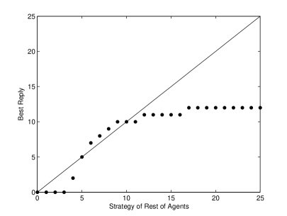
Figure 1: A hypothetical best-reply function with one type of agent.

There is a subtlety in our results. In general, there may be many equilibria. From the perspective of social welfare, some will be better than others. As we show in Section 5, strategies that use smaller (but nonzero) thresholds increase social welfare. Consider the best-reply function with a single type of agent shown in shown in Figure 1. An equilibrium must have $\mathit{BR}(k)=k$, so will be a point on the line $y=x$. This example has three equilibria: $S_{0}$, $S_{5}$, and $S_{10}$; $S_{5}$ is the equilibrium that maximizes social welfare. However, we cannot use best-reply dynamics to get to $S_{5}$, unless we start there. Applying best-reply dynamics to a starting point above 10 will lead to convergence at $S_{10}$; this is also true if we start at a point between 5 and 10. On the other hand, starting at a point below 5 will lead to convergence at $S_{0}$, the trivial equilibrium. Thus, although $S_{5}$ is a more efficient equilibrium than $S_{10}$, it is unstable. The only equilibrium that we can guarantee is stable is the maximum one (i.e., the greatest fixed point); thus, we focus on this equilibrium in the rest of the paper.

4 Identifying User Strategies

In Section 3, we used maximum entropy to get an explicit formula for the distribution of money given the fraction $\pi_{k}$ of agents using each strategy $S_{k}$, $k\geq 0$: $M^{k}_{i}=\pi_{k}\lambda^{i}/\sum_{j=0}^{k}\lambda^{j}$. In this section, we want to go in the opposite direction: given the distribution of money, we want to infer the fraction $f_{k}$ of agents using each strategy $S_{k}$, for each $k$. For those interested in studying the agents of a scrip system, knowing the fraction of agents using each strategy can provide a window into the preferences of those agents. For system designers, this knowledge is useful because, as we show in Section 5, how much money the system can handle without crashing depends on the fraction of agents of each type. In equilibrium, the distribution of money has the form described in Corollary 2. Note that in general we do not expect to see exactly this distribution at any given time, but it follows from Theorem 3.1 that, after sufficient time, the distribution is unlikely to be very far from it. Does this distribution help us identify the population? Without further constraints, it does not. Say that a distribution of money $M$ (where $M_{i}$ is the fraction of agents with $i$ dollars) is fully supported if there do not exist $i$ and $j$ such that $i<j$, $M_{j}>0$, and $M_{i}=0$. As the following lemma shows, a fully supported distribution can be explained in an infinite number of different ways. We take an “explanation” of $M$ (which has average amount of money $m$) to consist of a distribution $\vec{\pi}$ over strategies such that if a $\pi_{k}$ fraction of agents use strategy $S_{k}$ then $M^{*}_{\vec{\pi},m}=M$ (i.e., the maximum entropy distribution that results from those strategies will be $M$).

Lemma 6.

If $M$ is a fully supported distribution of money with finite support, there there exist an infinite number of explanations of $M$.

Proof 4.1.

Fix a value of $\lambda$. Then $M$ and $\lambda$ determine a distribution $\vec{\pi}$ as follows. Suppose that $k$ is the maximum amount of money that any agent has under $M$ (this is well defined since the support of $M$ is finite, by assumption). Then we take $\pi_{k}$ to be the unique value that satisfies

$$M_{k}=\pi_{k}\lambda^{k}/(\sum_{i=0}^{k}\lambda^{i}).$$

Note that $M_{j}=\sum_{i}M_{j}^{i}$. Therefore, once we have defined $\pi_{k}$, we can take $\pi_{k-1}$ to be the unique value that satisfies

$$M_{k-1}=\pi_{k}\lambda^{k-1}/(\sum_{i=0}^{k}\lambda^{i})+\pi_{k-1}\lambda^{k-1}/(\sum_{i=0}^{k-1}\lambda^{i}).$$

Iterating this process uniquely defines $\vec{\pi}$. However, $\vec{\pi}$ may not be a valid explanation, since some $\pi_{j}$ may be negative. This happens exactly when

$$M_{j}<\sum_{l=j+1}^{k}\pi_{l}\lambda^{j}/(\sum_{i=0}^{l}\lambda^{i}).$$

As $\lambda$ grows large, the terms on the right side of this inequality all tend towards 0. Thus, taking $\lambda$ sufficiently large ensures that $\pi_{j}\geq 0$ for all $j$. By construction, these values of $\pi_{j}$ are of a form that satisfied constraints (1) and (2), so $\pi$ is a valid explanation for $M$. Continuing to increase $\lambda$ will give an infinite number of different explanations.

We have not yet shown that there are types of agents for which the strategies in a given explanation are the strategies used in equilibrium. However, by examining the decision problem that determines the optimal threshold strategy for an agent, it can be shown that the parameters $\alpha$, $\gamma$, and $\delta$ can be set so as to make any threshold strategy optimal.

Lemma 7.

Let $M$ be the distribution of money in a nontrivial system and $\vec{\pi}$ be an explanation for $M$. Then for all $\beta>0$, $\rho>0$, and $k$, there exist $\alpha$, $\gamma$, and $\delta$ such that $S_{k}$ is the best reply for an agent of type $(\alpha,\beta,\gamma,\delta,\rho)$ to $\vec{\pi}$.

Proof 4.2.

(Sketch) Consider the decision problem faced by an agent when comparing $S_{i}$ to $S_{i+1}$. $S_{i}$ and $S_{i+1}$ differ only in what they do when an agent has $i$ dollars. As Theorem 4.1 of [4] shows, to decide whether or not to volunteer if he has $\$i$, an agent should determine the expected value of having a request satisfied when he runs out of money if he has $i$ dollars and plays $S_{i}$, and volunteer if this value is greater than $\alpha$. The parameters of the random walk that determines this expectation are determined by $i$, $M$, and $\vec{\pi}$. We can make $S_{k}$ optimal by fixing some $\alpha$ and $\gamma$ and then adjusting $\delta$ so that not working becomes superior exactly at $i=k+1$.

Lemma 6 shows that $M$ has an infinite number of explanations. Lemma 7 shows that we can find an equilibrium corresponding to each of them. Given an explanation $\vec{\pi}$, we can use Lemma 7 to find a type $t_{j}$ for which strategy $S_{j}$ with $j$ in the support of $\vec{\pi}$ is the best reply to $M$ and $\vec{\pi}$. Taking $T=\{t_{j}~{}|~{}j\in supp(\vec{\pi})\}$ and $f_{j}=\pi_{j}$ gives us a population for which $M$ is the equilibrium distribution of money. This type of population seems unnatural; it requires one type for each possible amount of money. We are typically interested in a more parsimonious explanation, one that requires relatively few types, for reasons the following lemma makes clear.

Lemma 8.

Let $\vec{\pi}$ be the true explanation for $M$. If $k$ is the largest threshold in the support of $\vec{\pi}$ and $s$ is the size of the support of $\vec{\pi}$, then any other explanation will have a support of size at least $k-s$.

Proof 4.3.

We know that $M^{k}_{i}=\pi_{k}\lambda^{i}/\sum_{j=0}^{k}\lambda^{j}$, where $\lambda$ is the (unique) value that satisfies constraint (1). Let $b_{k}=\pi_{k}/\sum_{j=0}^{k}\lambda^{j}$; then $M_{i}^{k}=\lambda^{i}b_{k}$, and $M_{i}=\sum_{k}M_{i}^{k}=B_{i}\lambda^{i}$, where $B_{i}=\sum_{k\geq i}b_{k}$. Note that if $\pi_{i-1}=0$, then $B_{i}=B_{i-1}$, so $M_{i}/M_{i-1}=\lambda$. Since $s$ strategies get positive probability according to $\vec{\pi}$, at least $k-s$ of the ratios $M_{i}/M_{i-1}$ with $1\leq i\leq k$ must have value $\lambda$. Any other explanation will have a different value $\lambda^{\prime}$ satisfying constraint (1). This means that the $k-s$ ratios with value $\lambda$ must correspond to places where $\pi_{i}>0$. Thus the support of any other explanation must be at least $k-s$.

If $s\ll k$, Lemma 8 gives us a strong reason for preferring the minimal explanation (i.e., the one with the smallest support); any other explanation will involve significantly more types. For $s=3$ and $k=50$, the smallest explanation has a support of at most three thresholds, and thus requires three types; the next smallest explanation requires at least 47 types. Thus, if the number of types of agents is relatively small, the minimal explanation will be the correct one. The proof of Lemma 8 also gives us an algorithm for finding this minimal explanation. We know that $M_{i}=B_{i}\lambda^{i}$. Therefore $\log M_{i}=\log B_{i}+i\log\lambda$. This means that in a plot of $\log M_{i}$, ranges of $i$ where $S_{i}$ is not played will be a line with slope $\lambda$. Thus, the minimal explanation can be found by finding the minimum number of lines of constant slope that fit the data. For a simple example of how such a distribution might look, Figure 2 shows an equilibrium distribution of money for the population

$$(\{(.05,1,1,.95,1),(.15,1,1,.95,1)\},(.3,.7),1000)$$

(i.e., the only difference between the types is it costs the second type three times as much to satisfy a request) with $m=4$ and the equilibrium strategies $(20,13)$. Figure 3 has the same distribution plotted on a log scale. Note the two lines with the same slope ($\lambda$) and the break at 14.

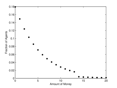
Figure 2: Distribution of money with two types of agents.

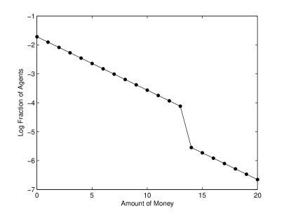
Figure 3: Log of the distribution of money with two types of agents.

Now we have an understanding of how we can take a distribution of money and infer from it the minimal explanation of the number of types of agents, the fraction of the population composed of each type, and the strategy each type is playing. (Note that we cannot distinguish multiple types playing the same strategy.) We would like to use this information to learn about the preferences of agents. The key observation is that the strategy chosen by an agent will be a best reply to the strategies of the other agents. The proof of Lemma 7 shows that from $M$ and $\vec{\pi}$ we can compute the parameters that control the random walk taken by an agent playing strategy $S_{k}$ starting with $k$ dollars until he runs out of money. This enables us to compute the expected stopping time of the random walk and, from this, a type for which $S_{k}$ is a best reply. This argument gives us constraints on the set of types for which $S_{k}$ is optimal. These constraints still allow quite a few possible types. However, suppose that over time $T$, the set of types, remains constant but $\vec{f}$, $n$, and $m$ all vary as agents join and leave the system. A later observation with a slightly different population (but the same $T$) would give another equilibrium with new constraints on the types of the agents. A number of such observations potentially reveal enough information to allow strong inferences about agent types. Thus far we have implicitly assumed that there are only a small number of types of agents in a system. Given that a type is defined by five real numbers, it is perhaps more reasonable to assume that each agent has a different type, but there is a small number of “clusters” of agents with similar types. For example, we might believe that generally agents either place a high value or a low value on receiving service. While the exact value may vary, the types of two low-value agents or two high-value agents will be quite similar. We have also assumed in our analysis that all agents play their optimal threshold strategy. However, computing this optimum may be too difficult for many agents. Even ignoring computational issues, agents may have insufficient information about their exact type or the exact types of other agents to compute the optimal threshold strategy. Assuming that there are a few clusters of agents with similar, but not identical, types and/or assuming that agents do not necessarily play their optimal threshold strategy, but do play a strategy close to optimal both lead to a similar picture of a system, which is one that we expect to see in practice: we will get clusters of agents playing similar strategies (that is, strategies with thresholds clustered around one value), rather than all agents in a cluster playing exactly the same strategy. This change has relatively little impact on our results. Rather than seeing straight lines representing populations with a sharp gap between them, as in Figure 3, we expect slightly curved lines representing a cluster of similar populations, with somewhat smoother transitions.

5 Optimizing the money supply

In Section 4 we considered how money is distributed among agents of different types, assuming that the money supply is fixed. We now want to examine what happens to the distribution of money as the amount of money changes. In particular, we want to determine the amount that optimizes the performance of the system. We will show that increasing the amount of money improves performance up to a certain point, after which the system experiences a monetary crash. Once the system crashes, the only equilibrium will be the trivial one where all agents play $S_{0}$. Thus, optimizing the performance of the system is a matter of finding out just how much money the system can handle before it crashes. Before we can start talking about optimal money supply, we have to answer a more fundamental question: given an equilibrium, how good is it? Consider a single round of the game with a homogeneous population of some fixed type $t$. If a request is satisfied, social welfare increases by $\gamma_{t}-\alpha_{t}$; the requester gains $\gamma_{t}$ utility and the satisfier pays a cost of $\alpha_{t}$. If no request is satisfied then no utility is gained. What is the probability that a request will be satisfied? This requires two events to occur. First, the agent chosen to make a request must have a dollar, which happens with probability $1-M_{0}$. Second, there must be a volunteer able and willing to satisfy the request. Any agent who does not have his threshold amount of money is willing to volunteer. Thus, if $\tau$ is the fraction of agents at their threshold then the probability of having a volunteer is $1-(1-\beta_{t})^{(1-\tau)n}$. We believe that in most large systems this probability is quite close to 1; otherwise, either $\beta_{t}$ must be unrealistically small or $\tau$ must be very close to 1. For example, even if $\beta=.01$ (i.e., an agent can satisfy 1% of requests), 1000 agents will be able to satisfy 99.99% of requests. If $\tau$ is close to 1, then agents will have an easier time earning money then spending money (the probability of spending a dollar is at most $1/n$, while for large $\beta$ the probability of earning a dollar if an agent volunteers is roughly $(1/n)(1/(1-\tau))$). If an agent is playing $S_{4}$ and there are $n$ rounds played a day, this means that for $\tau=.9$ he would be willing to pay $\alpha$ today to receive $\gamma$ over 10 years from now. For most systems, it seems unreasonable to have $\delta$ or $\gamma/\alpha$ this large. Thus, for the purposes of our analysis, we approximate $1-(1-\beta_{t})^{(1-\tau)n}$ by 1. With this approximation, we can write the expected increase in social welfare each round as $(1-M_{0})(\gamma_{t}-\alpha_{t})$. Since we have discount factor $\delta_{t}$, the total expected social welfare summed over all rounds is $(1-M_{0})(\gamma_{t}-\alpha_{t})/(1-\delta_{t})$. For heterogeneous types, the situation is essentially the same. Our equation for social welfare is more complicated because now the gain in welfare depends on the $\gamma$, $\alpha$, and $\delta$ of the agents chosen in that round, but the overall analysis is the same, albeit with more cases. Thus our goal is clear: find the amount of money that, in equilibrium, minimizes $M_{0}$. Many of the theorems in Section 3 begin “For all $m$ there exist $\delta^{*}$ and $n^{*}$ such that if $(T,\vec{f},n)$ is a payoff-heterogeneous population with $n>n^{*}$ and $\delta_{t}>\delta^{*}$ for all $t$”. Intuitively, the theorems require large $\delta_{t}$s to ensure that agents are patient enough that their decisions are dominated by long-run behavior rather than short-term utility, and large $n$ to ensure that small changes in the distribution of money do not move it far from the maximum-entropy distribution. In the following theorem and many of our later results, we want to assume that this condition is satisfied so that we can apply the theorems from Section 3. To simplify the statements of our theorems, we use “the standard conditions hold for $m$” to mean that the population $(T,\vec{f},n)$ under consideration is such that $n>n^{*}$ and $\delta_{t}>\delta^{*}$ for the $n^{*}$ and $\delta^{*}$ that the theorems require for $m$.

Theorem 9.

Let $(T,\vec{f},n)$ be a payoff-heterogeneous population such that the standard conditions hold for $m$ and $m^{\prime}$, $m<m^{\prime}$, and $\vec{k}$ is a nontrivial equilibrium for $(T,\vec{f},n)$ and $m$. Then if the average amount of money is $m^{\prime}$, best-reply dynamics starting at $\vec{k}$ will converge to some equilibrium $\vec{k}^{\prime}\leq\vec{k}$. Moreover, if $\vec{k}$ is the maximum equilibrium for $m$, then $\vec{k}^{\prime}$ is the maximum equilibrium for $m^{\prime}$. Furthermore, if $\vec{\pi}(\vec{k})$ is the distribution over strategies induced by $(T,\vec{f},n)$ and $\vec{k}$, and $\vec{k}^{\prime}$ is a nontrivial equilibrium, then $(M^{*}_{\vec{\pi}(\vec{k}^{\prime}),m^{\prime}})_{0}\leq(M^{*}_{\vec{\pi}(\vec{k}),m})_{0}$.

Proof 5.1.

(Sketch) Suppose that in the equilibrium with $m$, all agents of type $t$ use the threshold strategy $S_{k_{t}}$. Then $(M^{*}_{\vec{\pi}(\vec{k}),m})^{k}_{i}=\lambda_{m}^{i}/\sum_{j=0}^{k}\lambda_{m}^{j}$, where $\lambda_{m}$ is the value of that satisfies constraint (1) for $m$. It is relatively straightforward to show that if $m<m^{\prime}$, then $\lambda_{m}<\lambda_{m^{\prime}}$. If the equilibrium threshold strategy with both $m$ and $m^{\prime}$ were the same, then the desired result would be immediate. Unfortunately, changing the average amount of money may change the best-reply function. However, since $\lambda_{m^{\prime}}>\lambda_{m}$, it can be shown that $(M^{*}_{\vec{\pi}(\vec{k}),m^{\prime}})^{k_{t}}_{0}\leq(M^{*}_{\vec{\pi}(\vec{k}),m})^{k_{t}}_{k_{t}}$ and $(M^{*}_{\vec{\pi}(\vec{k}),m})^{k_{t}}_{k_{t}}\geq(M^{*}_{\vec{\pi}(\vec{k}),m})^{k_{t}}_{k_{t}}$, for all $k$ This increases the probability of an agent earning a dollar, so the best reply can only decrease. Thus, $\mathit{BR}_{(T,\vec{f}),m^{\prime}}(\vec{k})\leq\vec{k}$. Applying best-reply dynamics to $\mathit{BR}_{(T,\vec{f}),m^{\prime}}$ starting at $\vec{k}$, as in Theorem 5, gives us an equilibrium $\vec{k}^{\prime}$ such that $\vec{k}^{\prime}\leq\vec{k}$. Decreasing strategies only serves to further decrease $(M^{*}_{\vec{\pi}(\vec{k}^{\prime}),m^{\prime}})^{k_{t}^{\prime}}_{0}$, so as long as $\vec{k}$ is nontrivial we will have $(M^{*}_{\vec{\pi}(\vec{k}^{\prime}),m^{\prime}})_{0}\leq(M^{*}_{\vec{\pi}(\vec{k}),^{\prime}})_{0}$.

Theorem 9 makes several strong statements about what happens to social welfare as the amount of money increases (assuming there is no monetary crash). Taking the worst-case view, we know social welfare at the maximum equilibrium will increase. Alternatively, we can think of the system as being jolted out of equilibrium by a sudden addition of money. If agents react to this using best-reply dynamics and find a new nontrivial equilibrium, social welfare will have increased. In general, Theorem 9 suggests that, as long as nontrivial equilibria exist, the more money the better. As the following theorem shows, increasing the amount of money sufficiently leads to a monetary crash; moreover, once the system has crashed, adding more money does not make things better.

Corollary 10.

If $(T,\vec{f},n)$ is a payoff-heterogeneous population for which the standard conditions hold for $m$, then there exists a finite threshold $m_{T,\vec{f}}$ such that there exists a nontrivial equilibrium if the average amount of money is less than $m_{T,\vec{f}}$ and there does not exist a nontrivial equilibrium if the average amount of money is greater than $m_{T,\vec{f}}$. (A nontrivial equilibrium may or may not exist if the average amount of money is exactly $m_{T,\vec{f}}$.)

Proof 5.2.

Fix $(T,\vec{f},n)$. To see that there is some average amount of money $m$ for which there is no nontrivial equilibrium in this population, consider any average amount $m$. If there is no nontrivial equilibrium with $m$, then we are done. Otherwise, suppose the maximum equilibrium with $m$ is $\vec{k}_{m}$. Let $\vec{k}$ be such that $\mathit{BR}^{t}_{T,\vec{f},m}(\infty,\ldots,\infty)=k_{t}$. We must have $\vec{k}_{m}\leq\vec{k}$. Choose $m^{\prime}>\sum_{t}f_{t}k_{t}$. Suppose that the maximum equilibrium with $m^{\prime}$ is $\vec{k}_{m^{\prime}}$. By Theorem 9, we must have $\vec{k}_{m^{\prime}}\leq\vec{k}_{m}$. Thus, $\vec{k}_{m^{\prime}}\leq\vec{k}$. But if $\vec{k}_{m^{\prime}}$ is a nontrivial equilibrium, then in equilibrium, each agent of type $t$ has at most $k_{t}$ dollars, so the average amount of money in the system is at most $\sum_{t}f_{t}k_{t}<m^{\prime}$. Thus, there cannot be a nontrivial equilibrium if the average amount of money is $m^{\prime}$. Let $m_{T,\vec{f}}$ be the infimum over all $m$ for which no nontrivial equilibrium exists with population $(T,\vec{f},n)$ if the average amount of money is $m$. Clearly, by choice of $m_{T,\vec{f}}$, if $m<m_{T,\vec{f}}$, there is a nontrivial equilibrium. Now suppose that $m>m_{T,\vec{f}}$. By the construction of $m_{T,\vec{f}}$, there exists $m^{\prime}$ with $m>m^{\prime}>m_{T,\vec{f}}$ such that no nontrivial equilibrium exists if the average amount of money is $m^{\prime}$. Suppose, by way of contradiction, that there exists a nontrivial equilibrium if the average amount of money is $m$. Suppose that the maximum equilibrium is $\vec{k}$. By the same argument as that used in Theorem 9, the maximum equilibrium $\vec{k}^{\prime}$ if the average amount of money is $m^{\prime}$ is such that $\vec{k}^{\prime}>\vec{k}$. Thus, $\vec{k}^{\prime}$ is a nontrivial equilibrium.

Figure 4 shows an example of the monetary crash in a system with the same population used in Figure 2. Equilibria were found using best-reply dynamics starting at $(100,100)$.

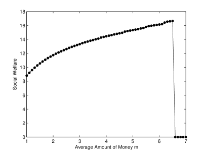
Figure 4: Social welfare for various average amounts of money, demonstrating a monetary crash.

In light of Corollary 10, the system designer should try to find $m_{T,\vec{f}}$. How can he do this? If he knows $T$ and $\vec{f}$, then he can perform a binary search for $m_{T,\vec{f}}$ by choosing values of $m$ and then using the algorithm from Section 3 to see if a nontrivial equilibrium exists. Observing the system over time and using the techniques described in Section 4 along with additional information he has about the system may be enough to make this a practical option. We expect a monetary crash to be a real phenomenon in a system where the price of servicing a request is fixed. This can be the case in practice, as shown by in the babysitting co-op example. If the price can change, we expect that as the money supply increases, there will be inflation; the price will increase so as to avoid a crash. However, floating prices can create other monetary problems, such as speculations, booms, and busts. Floating prices also impose transaction costs on agents. In systems where prices would normally be relatively stable, these transaction costs may well outweigh the benefits of floating prices.

6 Altruists and Hoarders

Thus far, we have considered standard agents with a type of the form $(\alpha,\beta,\gamma,\delta,\rho)$. We have a fairly complete picture of what happens in a system with only standard agents: increasing the money supply increases agent utility until a certain threshold is passed and the system has a monetary crash. However, any real system will have agents that, from perspective of the designer, behave oddly. These agents may be behaving irrationally or they may simply have a different utility function. For our results to be useful in practice, we need to understand how they are affected by such nonstandard agents. We consider here two such types of nonstandard agents, both of which have been observed in real systems: altruists and hoarders. Altruists, who provide service without requiring payment, reduce the incentive for standard agents to work. The end result is a decrease in the equilibrium threshold for standard agents. As a result, an excess of altruists, like an excess of money, can cause standard agents to stop being willing to work. However, up to the point where the system has a monetary crash, altruists improve the utility of standard agents. Hoarders, who want to collect as much money as possible whether it is actually useful or not, can be modeled as playing $S_{\infty}$. Since hoarders effectively absorb money, they make the remaining money more valuable, which increases the threshold used by standard agents in equilibrium. This results in reduced utility for standard agents, provided that the amount of money in the system is constant. Altruists may at first appear purely beneficial to standard agents, since they satisfy requests with no cost to standard agents. Indeed, as the following theorem shows, as long as the system does not have a monetary crash, altruists do make life better for standard agents. To show this, we assume that a fraction $a$ of requests get satisfied at no cost. Intuitively, these are the requests satisfied by the altruists, although the following result also applies to any setting where agents occasionally have a (free) outside option.

Theorem 11.

Consider a homogeneous population and assume that the standard conditions hold for $m$. Suppose that a fraction $a$ of requests can be satisfied at no cost. Then as long as the system does not have a monetary crash, social welfare increases as $a$ increases (assuming that the maximum equilibrium is always played).

Proof 6.1.

(Sketch) As we discussed in Section 5, the expected social welfare with a single type of standard agent is $(1-M_{0})(\gamma-\alpha)/(1-\delta)$. Rounds where a request is satisfied at no cost generate social welfare of $a\gamma/(1-\delta)$. The same analysis as in Section 5 shows that the remaining rounds generate social welfare of $(1-a)(1-M_{0}(a))(\gamma-\alpha)/(1-\delta)$, where $M_{0}(a)$ is the new equilibrium value of $M_{0}$ given that a fraction $a$ of requests are satisfied at no cost. Thus, the total welfare as a function of $a$ is

$$a\gamma/(1-\delta)+(1-a)(1-M_{0}(a))(\gamma-\alpha)/(1-\delta).$$

To see that this increases as $a$ increases, we would like to take the derivative relative to $a$ to get $(\gamma+(\gamma-\alpha)(-M_{0}^{\prime}(a)(1-a)-(1-M_{0}(a))))/(1-\delta)$. Unfortunately $M_{0}(a)$ may not even be continuous. Because strategies are integers, there will be regions where $M_{0}(a)$ is constant, and then a jump when a critical value of $a$ is reached that causes the equilibrium to change. In those regions where $M_{0}(a)$ is constant, $M_{0}^{\prime}(a)$ is 0. Since $1/(1-\delta)(\gamma+(\gamma-\alpha)(-(1-M_{0}(a))))$ is positive, social welfare is increasing in these regions. At points where $M_{0}(a)$ jumps, the equilibrium strategies will decrease. The proof of Theorem 9 shows that this decreases the value of $M_{0}(a)$ (unless the system crashes). This means that social welfare also increases at these points, so social welfare will always increase unless the system crashes.

Theorem 11 shows that altruists do not hurt provided that there are not enough them to crash the monetary system. But what if there are enough to crash the monetary system? As Adar and Huberman adar00 observed, this is essentially what has happened in Gnutella, where 70% of agents do not share any files, and nearly 50% of responses are from the top 1% of sharing hosts. In cases like this, whether standard agents are better off depends on the parameters of the system; the altruists may be satisfying fewer requests than would be satisfied in a cooperative equilibrium, but they are also not imposing the cost of satisfying these requests on the standard agents. Turning to hoarders, it seems in practice that whenever a system allows agents to accumulate something, be it work done, as in Seti@home, friends on online social networking sites, or “gold” in an online game, a certain group of agents seems to make it their goal to accumulate as much of it as possible. In pursuit of this, they will engage in behavior that seems irrational. For simplicity here, we model hoarders as playing the strategy $S_{\infty}$. This means that they will volunteer under all circumstances. Our analysis would not change significantly if we also required that they never made a request for work. Our first result shows that, for a fixed money supply, having more hoarders makes standard agents worse off.

Theorem 12.

Suppose that the standard agents in a system are described by $(T,\vec{f})$. Let $f_{H}$ be the fraction of hoarders (i.e., with probability $f_{H}$ an agent is a hoarder and with probability $1-f_{H}$ he is described by $(T,\vec{f},n)$). Assume that $(T,\vec{f},n)$ satisfies the standard conditions for $m$. Then, as $f_{H}$ increases, the utility of standard agents in the maximum equilibrium decreases.

Proof 6.2.

(Sketch) Increasing $f_{H}$ is equivalent to taking some number of standard agents and increasing their strategy to $S_{\infty}$. Lemma 4 shows us that the thresholds in equilibrium do not decrease. It can be shown by examining the formula for the maximum-entropy distribution that increasing strategies increases $M_{0}$. As the discussion in Section 5 shows, this will decrease agent utility.

Both Theorem 11 and 12 assume that the average amount of money in the system remains constant. However, the actions of both hoarders and altruists are visible to a system designer. The designer can take their existence into account when setting the money supply. As a general guideline, altruists require that money be removed from the system while hoarders require that it be added. Hoarders also have a beneficial aspect. As we have observed, a monetary crash occurs when a dollar becomes valueless because there are no agents willing to take it. However, with hoarders in the system, there is always someone to take it. Suppose that every standard agent in a system with hoarders plays $S_{0}$. As we saw in Lemma 7, we can compute the expected utility for having a single dollar and playing $S_{1}$. As long as this utility is greater than $\alpha$, the best reply will be greater than $S_{0}$. From Theorem 5, it follows that there will be a nontrivial equilibrium. Therefore, by Theorem 9, increasing $m$ will always increase social welfare. In practice, this seems like an unrealistic outcome. It seems likely that hoarders hoard only if money is seen as a scarce resource. Thus, as a practical matter, there is likely to be a limit to how far the system designer can increase $m$.

7 Conclusions and Future Work

For our model of a scrip system with payoff-heterogeneous types, we have proved that equilibria exist in threshold strategies and that the distribution of money in these equilibria is given by maximum entropy. As part of our equilibrium argument, we showed that the best-reply function is monotone. This proves the existence of equilibria in pure strategies and permits efficient algorithms to compute these equilibria. We have also examined some of the practical implications of these theoretical results. For someone interested in studying the agents of scrip systems, our characterization of equilibrium distribution of money forms the basis for techniques relevant to inferring characteristics of the agents of a scrip system from the distribution of money. For a system designer, our results on optimizing the money supply provide a simple maxim: keep adding money until the system is about to experience a monetary crash. Finally, we provide insight into the effects of altruists and hoarders on a scrip system, as well as providing guidance to system designers for dealing with them. There remain a number of interesting areas for future work, including the following:

• Our theoretical results all assume that agents are merely payoff heterogeneous. Varying $\beta$ or the request rate poses a problem for our techniques because the stationary distribution of the Markov chain will no longer be uniform, so we can no longer describe the equilibrium distribution of money using maximum entropy. However, there is nothing about this type of heterogeneity that intuitively poses a problem for convergence or threshold strategies. Indeed, we would expect that, knowing the average amount of money for one particular type, the distribution of money within that type should still follow a maximum-entropy distribution, because of the uniformity within the type. This would lead to a distribution of money that has a similar form, although now each type would have a different value of $\lambda$. If this is the case, many of our results still hold.

• It seems unlikely that altruism and hoarding are the only two types of “irrational” behavior we will find in real systems. Are there other major types that our model can provide insight into?

• It seems natural that the behavior of a very small group of agents should not be able to change the overall behavior of the system. Can we prove results about equilibria and utility when a small group follows an arbitrary strategy? This is particularly relevant when modeling attackers. See [1] for general results in this setting.

• Our model makes a number of strong predictions about the agent strategies, distribution of money, and effects of variations in the money supply. It also provides techniques to help analyze characteristics of agents of a scrip system. It would be interesting to test these predictions on a real functioning scrip system to either validate the model or gain insight from where its predictions are incorrect.

• What happens if we allow prices to vary over time, and have $\alpha$ and $\gamma$ varying by round as in the work of Hens et al. [6]. In this setting threshold strategies still seem natural to determine whether to work, but now the threshold would have to be a function of $\alpha$ and the payment that would be received rather than a constant. Furthermore, agents may wish to not make a request at all (even if they have the money to pay for it) if $\gamma$ is too small or the cost is too large. Again, we would expect to see thresholding behavior in these strategies.

Acknowledgements

We would like to thank Dan Reeves, Randy Farmer, and others at Yahoo! research for helpful discussions about applications of scrip systems and three anonymous referees for helpful suggestions. EF, IK and JH are supported in part by NSF under grant ITR-0325453. JH is also supported in part by NSF under grant IIS-0534064 and by AFOSR under grant FA9550-05-1-0055.

References

- [1] I. Abraham, D. Dolev, R. Gonen, and J. Halpern. Distributed computing meets game theory: Robust mechanisms for rational secret sharing and multiparty computation. pages 53–62, 2006.
- [2] E. Adar and B. A. Huberman. Free riding on Gnutella. First Monday, 5(10), 2000.
- [3] B. Chun, P. Buonadonna, A. AuYung, C. Ng, D. Parkes, J. Schneidman, A. Snoeren, and A. Vahdat. Mirage: A microeconomic resource allocation system for sensornet testbeds. In IEEE Workshopn on Embedded Networked Sensors, 2005.
- [4] E. J. Friedman, J. Y. Halpern, and I. Kash. Efficientcy and Nash equilibria in a scrip system for P2P networks. In J. Feigenbaum, J. Chuang, and D. Pennock, editors, ACM Conference on Electronic Commerce (EC), pages 140–149, 2006.
- [5] M. Gupta, P. Judge, and M. H. Ammar. A reputation system for peer-to-peer networks. In Network and Operating System Support for Digital Audio and Video (NOSSDAV), pages 144–152, 2003.
- [6] T. Hens, K. R. Schenk-Hoppe, and B. Vogt. The great Capitol Hill babysitting co-op: Anecdote or evidence for the optimum quantity of money? J. of Money, Credit and Banking, forthcoming. \balancecolumns
- [7] J. Ioannidis, S. Ioannidis, A. D. Keromytis, and V. Prevelakis. Fileteller: Paying and getting paid for file storage. In Financial Cryptography, pages 282–299, 2002.
- [8] Ithaca Hours Inc. Ithaca hours, 2005. http://www.ithacahours.org/.
- [9] E. T. Jaynes. Where do we stand on maximum entropy? In R. D. Levine and M. Tribus, editors, The Maximum Entropy Formalism, pages 15–118. MIT Press, Cambridge, Mass., 1978.
- [10] P. Krugman. The Accidental Theorist. Norton, 1999.
- [11] P. Milgrom and J. Roberts. Rationalizability, learning, and equilibrium in games with strategic complementarities. Econometrica, 58(6):1255–1277, 1900.
- [12] M. S. Miller and K. E. Drexler. Markets and computation: Agoric open systems. In B. Huberman, editor, The Ecology of Computation. Elsevier, 1988.
- [13] V. Pareto. Cours d’Economique Politique, vol. 2. Macmillan, 1897.
- [14] D. M. Reeves, B. M. Soule, and T. Kasturi. Group decision making with Yootles. http://ai.eecs.umich.edu/people/dreeves/yootles/yootles.pdf.
- [15] M. Stonebraker, P. M. Aoki, W. Litwin, A. Pfeffer, A. Sah, J. Sidell, C. Stelin, and A. Yu. Mariposa: a wide-area distributed database system. VLDB, 5(1):48–63, 1996.
- [16] J. Sweeney and R. J. Sweeney. Monetary theory and the great capitol hill babysitting co-op crisis: Comment. J. of Money, Credit and Banking, 9(1):86–89, 1977.
- [17] A. Tarski. A lattice-theoretical fixpoint theorem and its applications. Pacific Journal of Mathematics, 5:285–309, 1955.
- [18] R. H. Timberlake. Private production of scrip-money in the isolated community. J. of Money, Credit and Banking, 19(4):437–447, 1987.
- [19] D. M. Topkis. Equilibrium points in nonzero-sum n-person submodular games. Siam Journal of Control and Optimization, 17:773–787, 1979.
- [20] V. Vishnumurthy, S. Chandrakumar, and E. Sirer. Karma: A secure economic framework for peer-to-peer resource sharing. In Workshop on Economics of Peer-to-Peer Systems (P2PECON), 2003.
- [21] Washington Metropolitan Area Transit Commission. Scrip system of the D.C. transit system, 1970.