Dynamical models with a general anisotropy profile

Abstract

Aims. Both numerical simulations and observational evidence indicate that the outer regions of galaxies and dark matter haloes are typically mildly to significantly radially anisotropic. The inner regions can be significantly non-isotropic, depending on the dynamical formation and evolution processes. In an attempt to break the lack of simple dynamical models that can reproduce this behaviour, we explore a technique to construct dynamical models with an arbitrary density and an arbitrary anisotropy profile.

Methods. We outline a general construction method and propose a more practical approach based on a parameterized anisotropy profile. This approach consists of fitting the density of the model with a set of dynamical components, each of which have the same anisotropy profile. Using this approach we avoid the delicate fine-tuning difficulties other fitting techniques typically encounter when constructing radially anisotropic models.

Results. We present a model anisotropy profile that generalizes the Osipkov-Merritt profile, and that can represent any smooth monotonic anisotropy profile. Based on this model anisotropy profile, we construct a very general seven-parameter set of dynamical components for which the most important dynamical properties can be calculated analytically. We use the results to look for simple one-component dynamical models that generate simple potential-density pairs while still supporting a flexible anisotropy profile. We present families of Plummer and Hernquist models in which the anisotropy at small and large radii can be chosen as free parameters. We also generalize these two families to a three-parameter family that self-consistently generates the set of Veltmann potential-density pairs. These new analytical models are an important step forward compared to isotropic or Osipkov-Merritt models and can be used to generate the initial conditions for realistic simulations of galaxies or dark matter haloes.

1 Introduction

Numerical simulations, in particular $N$-body or hydrodynamical simulations, have become a major tool to study the structure, dynamics, stability and evolution of stellar systems and dark matter haloes. While at first sight this might seem to imply that analytical studies of spherically symmetric dynamical models have become less interesting, actually the opposite conclusion should be made. The construction of realistic and simple dynamical models is utterly important, as these models act as a reference frame or starting point from which to generate the initial conditions for numerical simulations. In this context, it is important to stress that the initial conditions need to be generated from the correct distribution function $F({\boldsymbol{r}},{\boldsymbol{v}})$ which completely determines the dynamical model. Kazantzidis et al. (2004) have recently demonstrated that the correct details of the velocity distribution should be taken into account. Simple ad-hoc Jeans dynamical models, i.e. models in which the kinematics are assumed to be Gaussian distributions with velocity dispersions derived from solving the Jeans equation, are not sufficient and can lead to erroneous conclusions. The quest for analytical dynamical models, which are simple enough on the one hand and realistic enough on the other hand, is hence still important.

In the past few years, many dynamical models have been proposed that are generated by various spherically symmetric potential-density pairs. The early-days models mainly represented systems with a constant density core, such as the Plummer model or the isochrone sphere (Plummer 1911; Hénon 1960). It now appears that many dynamical systems such as galaxies and dark matter haloes contain a central density cusp; also for such models a number of representative potential-density pairs have been constructed and distribution function have been derived (Jaffe 1983; Hernquist 1990; Dehnen 1993; Tremaine et al. 1994; Hiotelis 1994; Zhao 1996; Baes & Dejonghe 2002, 2004; Buyle et al. 2007).

Although the construction of analytical distribution functions hence has continued to develop, most simple models still show an important shortcoming: usually the distribution function can only be derived under strict and unrealistic conditions on the anisotropy of the velocity distribution. For many potential-density pairs, analytical distribution functions have only been derived under the assumption of isotropy. In this case, the phase-space distribution function that supports any density profile can be found as a simple integration using the famous Eddington formula. There are a few popular generalizations of the simple isotropic case that lead to dynamical models with an anisotropic velocity dispersion. Distribution functions with a constant anisotropy profile can be generated with a formula that is very similar to the Eddington formula (Dejonghe 1986; Baes & Dejonghe 2004; An & Evans 2006a). Another special category are the Osipkov-Merritt models, engineered independently by Osipkov (1979) and Merritt (1985). In these essentially one-dimensional models, the distribution function depends on the energy and angular momentum integrals only through a linear combination of both. The anisotropy profile for these models is peculiar in the sense that the velocity dispersion tensor is isotropic at small radii and becomes completely radial at large radii. The Osipkov-Merritt models were extended by Cuddeford (1991) to models in which the velocity dispersion tensor has an arbitrary anisotropy at small radii and becomes completely radial at large radii. The transition formulae for all these generalizations of the Eddington formula are sufficiently simple that analytical distribution functions of these kinds can be constructed for many simple potential-density pairs.

Whereas these models are a step beyond isotropic dynamical models, they still do not correspond to the anisotropy that is observed both in numerical simulations and real galaxies. Realistic dynamical systems typically have a tendency towards moderate to strong radial anisotropy at large radii. Cosmological simulations generally yield dynamical structures that are far from isotropic. Dark matter simulations in a cosmological CDM framework typically result in haloes in which the anisotropy gradually increases outward to levels of $\beta\approx 0.5$ at the virial radius (Cole & Lacey 1996; Colín et al. 2000; Fukushige & Makino 2001; Diemand et al. 2004). In general, there appears to be a connection between the logarithmic density slope $\gamma(r)={\text{d}}\ln\rho/{\text{d}}\ln r(r)$ and $\beta(r)$, both for pure dark matter haloes and for structures containing dark matter and baryons (Hansen & Moore 2006). This connection was argued to be a natural consequence of the Jeans equation (Dehnen & McLaughlin 2005) and it was shown numerically to be an attractor (Hansen & Stadel 2006).

In hydrodynamical simulations in which gas and stars are taken into account, galaxies also typically have a significant radial anisotropy at large radii (e.g. Oñorbe et al. 2007). Observational dynamical evidence appears to support these trends. For example, detailed stellar dynamical modelling of a large set of elliptical galaxies by Kronawitter et al. (2000) indicates that these galaxies generally contain an anisotropy profile that increases from near isotropy in the central regions towards a significant radial anisotropy at larger radii.

The anisotropy at small radii on the other hand is more subtle and depends largely on the dynamical processes that shape the nucleus of the system. In particular, the influence of a supermassive black hole, now believed to be present in nearly all hot stellar systems, can have a lasting influence on the central anisotropy. Models that contain a supermassive black hole that grows adiabatically by slow accretion of material are characterized by an isotropic to slightly tangential anisotropy profile in the central region with $\beta\sim-0.3$ (Quinlan et al. 1995). On the other hand, models with a binary supermassive black hole, formed by spiralling in due to dynamical friction, typically have much more outspoken tangential anisotropy in the central regions, with $\beta\sim-1$ (Quinlan & Hernquist 1997). This enhanced tangential anisotropy results from the preferential ejection of stars on radial orbits during the hardening of the black hole binary. Observationally, the study of the anisotropy profile at very small radii is difficult and hampered by both limited resolution effects and strong projection effects. Gebhardt et al. (2003) found that the most massive galaxies are strongly biased towards tangential orbits in the innermost regions, whereas the lower-mass galaxies have a range of central anisotropies.

From this body of evidence it is clear that we need to extend our set of simple isotropic or Osipkov-Merritt dynamical models to models in which the anisotropy profile has a more general shape, typically rising from isotropy or moderate tangential anisotropy at small radii to significant radial anisotropy at large radii. In the general anisotropic case, the transition formulae between density and distribution function are rather cumbersome (although mathematically elegant) and involve Laplace-Mellin integral transforms (Dejonghe 1986). The goal of the present paper is to describe a method to construct dynamical models with an arbitrary potential-density pair and an arbitrary anisotropy profile. We describe the general approach and the mathematical formulation in Section 2. In the next two sections we describe a more practical approach to construct such models: in Section 3 we propose a general parameterized anisotropy profile and in Section 4 we construct a general seven-parameter family of dynamical components based on this parameterized anisotropy profile for which the most important dynamical properties can be calculated analytically. In Section 5 we apply the results from the previous sections to construct a family of Plummer and Hernquist models with a smooth anisotropy profile with arbitrary values at small and large radii. We then extend these two families to a three-parameter family of generally anisotropic models that support the Veltmann set of potential-density pairs. Finally, our results are summarized in Section 6.

2 Construction of general anisotropic models

2.1 The augmented density formalism

In spherical symmetry, the distribution function depends only on two isolating integrals: the binding energy ${\mathcal{E}}$ and the magnitude of the angular momentum $L$ per unit mass,

$${\mathcal{E}}=\psi(r)-\tfrac{1}{2}\,v_{r}^{2}-\tfrac{1}{2}\,v_{T}^{2},$$ (1)

$$L=r\,v_{T}.$$ (2)

In these expressions $\psi(r)$ is the positive binding potential of the system, connected to the density through Poisson’s equation

$$\frac{1}{r^{2}}\,\frac{{\text{d}}}{{\text{d}}r}\left(r^{2}\,\frac{{\text{d}}\psi}{{\text{d}}r}\right)(r)=-4\pi G\rho(r).$$ (3)

and $v_{T}$ is the transverse velocity

$$v_{T}=\sqrt{v_{\theta}^{2}+v_{\varphi}^{2}}.$$ (4)

When we have an expression for the distribution function, all interesting dynamical properties can be derived. In particular, the moments of the distribution function can be calculated as

$$\mu_{2n,2m}(r)=2\pi M\iint F({\mathcal{E}},L)\,v_{r}^{2n}\,v_{T}^{2m+1}\,{\text{d}}v_{r}\,{\text{d}}v_{T}.$$ (5)

If we want to construct dynamical models for a given density profile in practice, it is easier to consider an alternative characterization of a spherical dynamical model, namely the framework of the augmented densities. An augmented density is a bivariate function $\tilde{\rho}(\psi,r)$, which expresses the density as an explicit function of both the radius $r$ and the gravitational potential $\psi$. One can demonstrate that each augmented density function $\tilde{\rho}(\psi,r)$ completely determines a distribution function $F({\mathcal{E}},L)$ and vice versa. There are several transition formulae between these two equivalent formalisms, including an elegant formalism based on combined Laplace-Mellin integral transforms.

One of the advantages of the augmented density formalism is that it is straightforward to construct self-consistent dynamical models that correspond to a given density profile. Indeed, we just have to solve Poisson’s equation, and construct any augmented density $\tilde{\rho}(\psi)$ that satisfies the relation

$$\rho(r)=\tilde{\rho}(\psi(r),r).$$ (6)

Obviously, there are always infinitely many augmented density functions that satisfy equation (6) for a given density profile $\rho(r)$. These different dynamical models have different moments of the distribution function, and we often are looking for those particular dynamical models which have a certain anisotropy profile, defined as

$$\beta(r)=1-\frac{\sigma_{T}^{2}(r)}{2\sigma_{r}^{2}(r)}.$$ (7)

It appears that the augmented density formalism of dynamical models is a very useful way to achieve this goal. Indeed, another advantage of this formalism is that the moments of the distribution function can be derived from the augmented density by subsequent derivations and a single integration,

$$\tilde{\mu}_{2n,2m}(\psi,r)=\frac{2^{m+n}}{\sqrt{\pi}}\,\frac{\Gamma\left(n+\tfrac{1}{2}\right)}{\Gamma\left(m+n\right)}\int_{0}^{\psi}\left(\psi-\psi^{\prime}\right)^{m+n-1}D_{r^{2}}^{m}\left[r^{2m}\tilde{\rho}(\psi^{\prime},r)\right]{\text{d}}\psi^{\prime},$$ (8)

where $D_{x}^{m}$ denotes the $m\,$th differentiation with respect to $x$. In particular, the radial and transverse velocity dispersions can be found from the density through the relations

$$\tilde{\sigma}_{r}^{2}(\psi,r)=\frac{\tilde{\mu}_{20}(\psi,r)}{\tilde{\mu}_{00}(\psi,r)}=\frac{1}{\tilde{\rho}(\psi,r)}\int_{0}^{\psi}\tilde{\rho}(\psi^{\prime},r)\,{\text{d}}\psi^{\prime},$$ (9)

$$\tilde{\sigma}_{T}^{2}(\psi,r)=\frac{\tilde{\mu}_{02}(\psi,r)}{\tilde{\mu}_{00}(\psi,r)}=\frac{2}{\tilde{\rho}(\psi,r)}\int_{0}^{\psi}D_{r^{2}}\left[r^{2}\,\tilde{\rho}(\psi^{\prime},r)\right]{\text{d}}\psi^{\prime}.$$ (10)

2.2 Construction of general anisotropic models

Now consider an augmented density that is a separable function of $\psi$ and $r$,

$$\tilde{\rho}(\psi,r)=f(\psi)\,g(r).$$ (11)

For such models, the dispersion profiles read

$$\tilde{\sigma}_{r}^{2}(\psi,r)=\frac{1}{f(\psi)}\int_{0}^{\psi}f(\psi^{\prime})\,{\text{d}}\psi^{\prime},$$ (12)

$$\tilde{\sigma}_{T}^{2}(\psi,r)=\left(1+\frac{1}{2}\frac{{\text{d}}\ln g}{{\text{d}}\ln r}\right)\frac{2}{f(\psi)}\int_{0}^{\psi}f(\psi^{\prime})\,{\text{d}}\psi^{\prime},$$ (13)

such that

$$\beta(r)=-\frac{1}{2}\frac{{\text{d}}\ln g}{{\text{d}}\ln r}(r).$$ (14)

For models with a separable augmented density, the radial velocity dispersion depends only on the $\psi$-dependent part of the augmented density, whereas the anisotropy depends only on the $r$-dependent part.

Equation (14) offers us in principle the opportunity to construct dynamical models with an arbitrary density profile $\rho(r)$ and an arbitrary anisotropy profile. First we solve equation (14) for $g(r)$. Next we determine the gravitational potential $\psi(r)$ by solving Poisson’s equation, we invert this relation as $r(\psi)$ and we set

$$\bar{g}(\psi)=g(r(\psi)),$$ (15)

$$\bar{\rho}(\psi)=\rho(r(\psi)),$$ (16)

$$f(\psi)=\frac{\bar{\rho}(\psi)}{\bar{g}(\psi)},$$ (17)

then the augmented density

$$\tilde{\rho}(\psi,r)=f(\psi)\,g(r)$$ (18)

defines the desired model.

2.3 Practical construction

Although we have defined a way to construct an augmented density for a dynamical model with an arbitrary density and anisotropy profile, this is of limited use in practice. Indeed, the quantity we really want is the distribution function for the model. In principle, the distribution function for each $\tilde{\rho}(\psi,r)$ can be recovered with the standard Laplace-Mellin integral transform formulae. However, the augmented density that results from an arbitrary choice of $\rho(r)$ and $\beta(r)$ will often be too complicated to allow an analytical integral transform. As a result, we have to compute the distribution function by numerical means. Unfortunately, the numerical inversion of equation (5) to obtain the distribution function from the augmented density is in general numerically unstable. Indeed, since the density is an integration of the distribution function over velocity space, the density is generally much smoother than the distribution function. The inversion procedure of determining $f$ from $\rho$ hence has the tricky job of unsmoothing the information contained in the smoothed density. It hence comes as no surprise that this operation is numerically unstable. For a more precise mathematical demonstration of the unstable character of the inversion formulae, we refer to Dejonghe (1986).

A more promising strategy is to determine a general parameterized model for $\beta(r)$ that leads to a relatively simple function $g(r)$. For each function $f(\psi)$, we can subsequently construct a dynamical model $\tilde{\rho}(\psi,r)$ that has the same anisotropy profile. Now consider a set of base functions $f_{\ell}(\psi)$ that are sufficiently simple such that the augmented density $\tilde{\rho}_{\ell}(\psi,r)=f_{\ell}(\psi)\,g(r)$ can be converted analytically to a distribution function $F_{\ell}({\mathcal{E}},L)$. It is easy to see that any linear combination of such dynamical models will again define a dynamical model with the same anisotropy profile since

$$\sum_{\ell}a_{\ell}\,\tilde{\rho}_{\ell}(\psi,r)=\left[\sum_{\ell}a_{\ell}\,f_{\ell}(\psi)\right]g(r).$$ (19)

So if we can find a suitable linear combination of the base functions such that

$$f(\psi)=\frac{\bar{\rho}(\psi)}{\bar{g}(\psi)}=\sum_{\ell}a_{\ell}\,f_{\ell}(\psi),$$ (20)

we immediately obtain the required distribution function

$$F({\mathcal{E}},L)=\sum_{\ell}a_{\ell}\,F_{\ell}({\mathcal{E}},L).$$ (21)

Finding the best linear combination of the components such that the condition (20) is satisfied can in principle be achieved by making a formal series expansion and determine each of the expansion coefficients for each component. In practice however, it is more straightforward to approximate the dynamical model by a $\chi^{2}$-minimization routine. This could for example be achieved by means of quadratic programming, in which a boundary condition is set that forces the distribution function to remain positive in the entire phase space. Practical realizations of this technique are already in use by various dynamical modellers (Dejonghe 1989; Kuijken & Merrifield 1993; Merrifield & Kuijken 1994; Gerhard et al. 1998).

The remaining steps we still have to take are hence (1) create a general parameterized anisotropy profile $\beta(r)$ that is flexible enough to represent an array of realistic anisotropy profiles and that still yields a simple $g(r)$ function, (2) provide a suitable set of base functions or components $f_{\ell}(\psi)$ for which, in combination with the $g(r)$ function derived above, the corresponding distribution function can be computed analytically. We will look into these two steps in the next two sections.

3 A parameterized anisotropy profile

As mentioned before, very few analytical dynamical models are known that have a realistic anisotropy profile. Most are either completely isotropic, have a constant anisotropy or have an anisotropy profile according to the Osipkov-Merritt type (isotropic in the centre and completely radially anisotropic at large radii). In this paper, we aim at the construction of spherical dynamical models with a more general and realistic anisotropy profile. The most realistic approach would involve an anisotropy profile that depends explicitly on the density slope, as described in the Introduction. However, this would in general not yield an augmented density that allows an analytical distribution function. Instead, we will create dynamical models with an anisotropy profile that is an explicit function of the radius $r$. As long as the anisotropy profiles have enough freedom, this will in practice enable us to construct dynamical models in which the anisotropy and density slope are at least qualitatively connected. Our specific goal is to create dynamical models in which the anisotropy changes monotonically from an arbitrary value $\beta_{0}$ at the central regions to another arbitrary value $\beta_{\infty}$ at large radii, without a priori limitations on the values of $\beta_{0}$ or $\beta_{\infty}$. To reach this goal, we need to provide a functional form that has the desired properties at small and large radii and that can be inverted to give a reasonable simple form for $g(r)$. Finding such a form for $\beta(r)$ is not obvious. A straightforward candidate that has the desired asymptotic behaviour is an exponential profile

$$\beta(r)=\beta_{\infty}-(\beta_{\infty}-\beta_{0})\exp\left(-\frac{r}{r_{\text{a}}}\right).$$ (22)

Solving for equation (14) yields, apart from an arbitrary normalization factor,

$$g(r)=\left(\frac{r}{r_{\text{a}}}\right)^{-2\beta_{\infty}}\exp\left[-2\,(\beta_{\infty}-\beta_{0})\operatorname{Ei}_{1}\left(\frac{r}{r_{\text{a}}}\right)\right].$$ (23)

It comes as no surprise that such a model will not result in a simple augmented density that can be inverted to an analytical distribution function. In order to find a more suitable candidate function for $\beta(r)$ we inspire ourselves on the Osipkov-Merritt models, where the anisotropy profile reads

$$\beta(r)=\frac{r^{2}}{r_{\text{a}}^{2}+r^{2}}=\frac{(r/r_{\text{a}})^{2}}{1+(r/r_{\text{a}})^{2}},$$ (24)

resulting in isotropy in the central regions and complete radial anisotropy at large radii. The resulting solution for $g(r)$ reads

$$g(r)=\left(1+\frac{r^{2}}{r_{\text{a}}^{2}}\right)^{-1}.$$ (25)

Cuddeford (1991) generalized the Osipkov-Merritt models by considering models with an anisotropy profile

$$\beta(r)=\frac{\beta_{0}+(r/r_{\text{a}})^{2}}{1+(r/r_{\text{a}})^{2}}.$$ (26)

These models also become completely radial at large radii, but at small radii they can assume an arbitrary anisotropy $\beta_{0}$. If we introduce this expression into equation (14) we obtain the relatively simple expression

$$g(r)=\left(\frac{r}{r_{\text{a}}}\right)^{-2\beta_{0}}\left(1+\frac{r^{2}}{r_{\text{a}}^{2}}\right)^{\beta_{0}-1}.$$ (27)

The obvious way to generalize these results such that the anisotropy does not have to become completely radial at large radii is to consider the profile

$$\beta(r)=\frac{\beta_{0}+\beta_{\infty}(r/r_{\text{a}})^{2}}{1+(r/r_{\text{a}})^{2}},$$ (28)

which corresponds to

$$g(r)=\left(\frac{r}{r_{\text{a}}}\right)^{-2\beta_{0}}\left(1+\frac{r^{2}}{r_{\text{a}}^{2}}\right)^{-(\beta_{\infty}-\beta_{0})}.$$ (29)

In fact, an even more general form for the anisotropy that yields a very similar $g$ function is

$$\beta(r)=\frac{\beta_{0}+\beta_{\infty}(r/r_{\text{a}})^{2\delta}}{1+(r/r_{\text{a}})^{2\delta}},$$ (30)

with $\delta>0$, which corresponds to

$$g(r)=\left(\frac{r}{r_{\text{a}}}\right)^{-2\beta_{0}}\left(1+\frac{r^{2\delta}}{r_{\text{a}}^{2\delta}}\right)^{\beta_{\delta}},$$ (31)

with

$${\beta_{\delta}}=\frac{\beta_{0}-\beta_{\infty}}{\delta}.$$ (32)

The couple (30)-(31) is a suitable choice for our goals. On the one hand this four-parameter model anisotropy contains enough flexibility to represent any monotonically varying anisotropy profile (with increasing or decreasing anisotropy). The parameters have straightforward effects: $\beta_{0}$ and $\beta_{\infty}$ set the anisotropy at small and large radii respectively, $r_{\text{a}}$ determines the typical transition radius between the two regimes and $\delta$ sets the sharpness by which this transition takes place. On the other hand, the resulting $g(r)$ function is sufficiently simple to lead to analytical dynamical components for suitably chosen $f(\psi)$ functions.

4 A library of components

The missing link in our approach is a set of base functions or components with which we can construct a linear combination. We need to look for functions $f_{\ell}(\psi)$ such that the augmented density

$$\tilde{\rho}_{\ell}(\psi,r)=f_{\ell}(\psi)\left(\frac{r}{r_{\text{a}}}\right)^{-2\beta_{0}}\left(1+\frac{r^{2\delta}}{r_{\text{a}}^{2\delta}}\right)^{\beta_{\delta}},$$ (33)

gives rise to an analytical distribution functions $F_{\ell}({\mathcal{E}},L)$. We will drop the subscript $\ell$ in the remainder of this section in order not to overload the notations.

4.1 Power law components

The most obvious candidate components are those in which $f(\psi)$ is a power law,

$$\tilde{\rho}(\psi,r)=\rho_{0}\left(\frac{\psi}{\psi_{0}}\right)^{p}\left(\frac{r}{r_{\text{a}}}\right)^{-2\beta_{0}}\left(1+\frac{r^{2\delta}}{r_{\text{a}}^{2\delta}}\right)^{\beta_{\delta}},$$ (34)

where we limit ourselves to systems with a finite potential well $\psi_{0}=\psi(0)$. A finite total mass is obtained if $p+2\beta_{\infty}>3$. In order to calculate the distribution function corresponding to this augmented density, we apply the general Mellin-Laplace inversion formulae. After some algebra (see Appendix A), we find that it can be expressed as a Fox $H$-function:

$$F({\mathcal{E}},L)=\frac{\rho_{0}}{M(2\pi\,\psi_{0})^{3/2}}\,\frac{\Gamma(1+p)}{\delta\,\Gamma(-{\beta_{\delta}})}\,\left(\frac{{\mathcal{E}}}{\psi_{0}}\right)^{p-3/2}\,H_{2,2}^{1,1}\left(\frac{L^{2}}{2r_{\text{a}}^{2}{\mathcal{E}}}\left|\,\begin{array}[]{r@{\,,\,}l}\left(1-\frac{\beta_{\infty}}{\delta},\frac{1}{\delta}\right)&\left(p-\frac{1}{2},1\right)\\[5.69054pt] \left(-\frac{\beta_{0}}{\delta},\frac{1}{\delta}\right)&\left(0,1\right)\end{array}\,\right.\right).$$ (35)

As we show in Appendix A, a sufficient (but not necessary) condition to yield a well-defined distribution function, i.e. continuous and non-negative, is $\delta<1$ or $\delta=1$ and $p-\frac{1}{2}+\beta_{\delta}>0$.

For practical purposes, a series expansion is more useful. After some lengthy algebra, one obtains the fairly simple expression (see Appendix B)

$$F({\mathcal{E}},L)=\frac{\rho_{0}\,\Gamma(1+p)}{M(2\pi\,\psi_{0})^{3/2}}\left(\frac{{\mathcal{E}}}{\psi_{0}}\right)^{p-3/2}\times\begin{cases}\;\displaystyle\sum_{k=0}^{\infty}\binom{{\beta_{\delta}}}{k}\,\dfrac{1}{\Gamma\left(1-\beta_{0}+k\delta\right)\Gamma\left(p-\frac{1}{2}+\beta_{0}-k\delta\right)}\,\left(\dfrac{L^{2}}{2r_{\text{a}}^{2}{\mathcal{E}}}\right)^{-\beta_{0}+k\delta}&\qquad\text{for }L^{2}<2r_{\text{a}}^{2}{\mathcal{E}},\\[16.99998pt] \;\displaystyle\sum_{k=0}^{\infty}\binom{{\beta_{\delta}}}{k}\,\dfrac{1}{\Gamma\left(1-\beta_{\infty}-k\delta\right)\Gamma\left(p-\frac{1}{2}+\beta_{\infty}+k\delta\right)}\,\left(\dfrac{L^{2}}{2r_{\text{a}}^{2}{\mathcal{E}}}\right)^{-\beta_{\infty}-k\delta}&\qquad\text{for }L^{2}>2r_{\text{a}}^{2}{\mathcal{E}}.\end{cases}$$ (36)

Apart from the distribution function, most other interesting dynamical properties can be calculated analytically for this set of components. Particularly simple are the velocity dispersions, which we find through (12),

$$\tilde{\sigma}_{r}^{2}(\psi,r)=\frac{\psi}{1+p},$$ (37)

$$\tilde{\sigma}_{\theta}^{2}(\psi,r)=\tilde{\sigma}_{\varphi}^{2}(\psi,r)=\frac{(1-\beta_{0})+(1-\beta_{\infty})\,(r/r_{\text{a}})^{2\delta}}{1+(r/r_{\text{a}})^{2\delta}}\,\tilde{\sigma}_{r}^{2}(\psi,r).$$ (38)

4.2 Extension to cuspy components

This set of power law components presented in the previous subsection is very adequate to fit a broad class of models. It is however, not fit to construct dynamical models for systems that have a central density cusp. For such models, the isotropic distribution function diverges in the limit ${\mathcal{E}}\rightarrow\psi_{0}$ (see e.g. Hernquist 1990; Dehnen 1993; Tremaine et al. 1994; Baes et al. 2005). This behaviour cannot be represented with the current set of components. Therefore we extend the set of models defined by the augmented density (34) to

$$\tilde{\rho}(\psi,r)=\rho_{0}\left(\frac{\psi}{\psi_{0}}\right)^{p}\,\left(1-\frac{\psi^{s}}{\psi_{0}^{s}}\right)^{q}\left(\frac{r}{r_{\text{a}}}\right)^{-2\beta_{0}}\left(1+\frac{r^{2\delta}}{r_{\text{a}}^{2\delta}}\right)^{\beta_{\delta}},$$ (39)

with two additional parameters $q\leqslant 0$ and $s>0$. This seven-parameter family of dynamical components contains enough freedom in the density profile to form a good family of base functions. If we expand this expression as a power series in $\psi$,

$$\tilde{\rho}(\psi,r)=\rho_{0}\sum_{j=0}^{\infty}(-1)^{j}\,\binom{q}{j}\left(\frac{\psi}{\psi_{0}}\right)^{p+js}\left(\frac{r}{r_{\text{a}}}\right)^{-2\beta_{0}}\left(1+\frac{r^{2\delta}}{r_{\text{a}}^{2\delta}}\right)^{\beta_{\delta}},$$ (40)

we see that we obtain a series of positive terms that all have the form (34). Thus, our condition $q\leqslant 0$ is sufficient to obtain a well-defined distribution function, which we can write down immediately,

$$F({\mathcal{E}},L)=\frac{\rho_{0}}{M(2\pi\,\psi_{0})^{3/2}}\,\sum_{j=0}^{\infty}(-1)^{j}\,\binom{q}{j}\,\frac{\Gamma(1+p+js)}{\delta\,\Gamma(-{\beta_{\delta}})}\,\left(\frac{{\mathcal{E}}}{\psi_{0}}\right)^{p+js-3/2}\,H_{2,2}^{1,1}\left(\frac{L^{2}}{2r_{\text{a}}^{2}{\mathcal{E}}}\left|\,\begin{array}[]{r@{\,,\,}l}\left(1-\frac{\beta_{\infty}}{\delta},\frac{1}{\delta}\right)&\left(p+js-\frac{1}{2},1\right)\\[5.69054pt] \left(-\frac{\beta_{0}}{\delta},\frac{1}{\delta}\right)&\left(0,1\right)\end{array}\,\right.\right),$$ (41)

or explicitly

$$F({\mathcal{E}},L)=\frac{\rho_{0}}{M(2\pi\,\psi_{0})^{3/2}}\,\sum_{j=0}^{\infty}(-1)^{j}\,\binom{q}{j}\,\Gamma(1+p+js)\left(\frac{{\mathcal{E}}}{\psi_{0}}\right)^{p+js-3/2}\\ \times\begin{cases}\;\displaystyle\sum_{k=0}^{\infty}\binom{{\beta_{\delta}}}{k}\,\dfrac{1}{\Gamma\left(1-\beta_{0}+k\delta\right)\Gamma\left(p+js-\frac{1}{2}+\beta_{0}-k\delta\right)}\,\left(\dfrac{L^{2}}{2r_{\text{a}}^{2}{\mathcal{E}}}\right)^{-\beta_{0}+k\delta}&\qquad\text{for }L^{2}<2r_{\text{a}}^{2}{\mathcal{E}},\\[16.99998pt] \;\displaystyle\sum_{k=0}^{\infty}\binom{{\beta_{\delta}}}{k}\,\dfrac{1}{\Gamma\left(1-\beta_{\infty}-k\delta\right)\Gamma\left(p+js-\frac{1}{2}+\beta_{\infty}+k\delta\right)}\,\left(\dfrac{L^{2}}{2r_{\text{a}}^{2}{\mathcal{E}}}\right)^{-\beta_{\infty}-k\delta}&\qquad\text{for }L^{2}>2r_{\text{a}}^{2}{\mathcal{E}}.\end{cases}$$ (42)

Since the summations in $j$ converge for every fixed value of $k$, this distribution function is indeed well-defined. Other dynamical properties, such as the moments of the distribution function, can be derived in the same way. For the velocity dispersions we find

$$\tilde{\sigma}_{r}^{2}(\psi,r)=\frac{\psi_{0}}{s}\left(\frac{\psi}{\psi_{0}}\right)^{-p}\left(1-\frac{\psi^{s}}{\psi_{0}^{s}}\right)^{-q}B_{\psi^{s}/\psi_{0}^{s}}\!\left(\frac{1+p}{s},1+q\right),$$ (43)

$$\tilde{\sigma}_{\theta}^{2}(\psi,r)=\tilde{\sigma}_{\varphi}^{2}(\psi,r)=\frac{(1-\beta_{0})+(1-\beta_{\infty})\,(r/r_{\text{a}})^{2\delta}}{1+(r/r_{\text{a}})^{2\delta}}\,\tilde{\sigma}_{r}^{2}(\psi,r),$$ (44)

with $B_{x}(a,b)$ the incomplete Beta function.

5 Self-consistent analytical models

In the previous Section we have described a practical method to construct analytical self-consistent dynamical models that generate any spherical density profile and with an anisotropy profile defined by the general parameterized function (30). We are applying this technique to construct dynamical models matching the density and anisotropy profiles that have come out of cosmological simulations of dark matter haloes, in order to gain insight into their phase-space structure (Van Hese, Baes & Dejonghe 2007). In the remainder of this current paper we will focus on simple analytical dynamical models, by investigating whether the global seven-parameter family of dynamical models defined by the augmented density (39) contains any simple self-consistent models (hence without the need to make a linear combination). Thus we will look for potential-density pairs $[\rho(r),\psi(r)]$ that satisfy both Poisson’s equation and the relation

$$\rho(r)=\tilde{\rho}(\psi(r),r),$$ (45)

with $\tilde{\rho}(\psi,r)$ the seven-parameter augmented density from equation (39). The existence of such analytical dynamical models would be a great step forward in our quest for simple but realistic dynamical models that can be used as a framework in which to initiate detailed numerical simulations.

5.1 A family of anisotropic Plummer models

One of the most obvious candidates is the Plummer model, as this model has a rather straightforward potential-density pair

$$\psi(r)=\frac{GM}{\sqrt{b^{2}+r^{2}}},$$ (46)

$$\rho(r)=\frac{3M}{4\pi b^{3}}\left(1+\frac{r^{2}}{b^{2}}\right)^{-5/2}.$$ (47)

When we combine these functions with the expressions (39) and (45), we obtain the condition

$$\frac{3M}{4\pi b^{3}}\left(1+\frac{r^{2}}{b^{2}}\right)^{-5/2}=\rho_{0}\left(1+\frac{r^{2}}{b^{2}}\right)^{-p/2}\left[1-\left(1+\frac{r^{2}}{b^{2}}\right)^{-s/2}\right]^{q}\left(\frac{r}{r_{\text{a}}}\right)^{-2\beta_{0}}\left(1+\frac{r^{2\delta}}{r_{\text{a}}^{2\delta}}\right)^{-(\beta_{\infty}-\beta_{0})/\delta}.$$ (48)

A straightforward solution is obviously given by

$$\rho_{0}=\frac{3M}{4\pi b^{3}},$$ (49)

$$p=5,$$ (50)

$$q=\beta_{0}=\beta_{\infty}=0,$$ (51)

which yields the isotropic Plummer model, defined by

$$\tilde{\rho}(\psi)=\frac{3M}{4\pi b^{3}}\,\left(\frac{b\psi}{GM}\right)^{5}.$$ (52)

$$F({\mathcal{E}})=\frac{3}{7\pi^{3}\,(GMb)^{3/2}}\left(\frac{2b{\mathcal{E}}}{GM}\right)^{7/2}.$$ (53)

Our goal, however, is to determine the most general subspace of the $(p,q,s,\beta_{0},\beta_{\infty},\delta,r_{\text{a}})$ parameter space such that the condition (48) is satisfied for all $r$. In particular we aim for a subspace of the parameter space that has no restrictions on $\beta_{0}$ and $\beta_{\infty}$, such that we obtain a family of dynamical models with an arbitrary anisotropy at small and large radii. It is obvious from equation (48) that, in order to find non-trivial solutions, we have to set

$$s=2\delta=2,$$ (54)

$$r_{\text{a}}=b.$$ (55)

We then obtain the expression

$$\frac{3M}{4\pi b^{3}\rho_{0}}\left(\frac{r^{2}}{b^{2}}\right)^{\beta_{0}-q}\left(1+\frac{r^{2}}{b^{2}}\right)^{-5/2+p/2+q+\beta_{\infty}-\beta_{0}}=1.$$ (56)

These expressions are identical for all values of $r$ if

$$\rho_{0}=\frac{3M}{4\pi b^{3}},$$ (57)

$$p=5-2\beta_{\infty},$$ (58)

$$q=\beta_{0}.$$ (59)

We now have constructed a general two-parameter family of self-consistent Plummer models with the augmented density profile

$$\tilde{\rho}(\psi,r)=\frac{3M}{4\pi\,b^{3}}\left(\frac{b\psi}{GM}\right)^{5-2\beta_{\infty}}\left[1-\left(\frac{b\psi}{GM}\right)^{2}\right]^{\beta_{0}}\left(\frac{r^{2}}{b^{2}}\right)^{-\beta_{0}}\left(1+\frac{r^{2}}{b^{2}}\right)^{-(\beta_{\infty}-\beta_{0})}.$$ (60)

From the condition $q\leqslant 0$ it follows that the central anisotropy has to satisfy $\beta_{0}\leqslant 0$. This is in fact a special case of the cusp slope-central anisotropy theorem of An & Evans (2006b): a model without a density cusp cannot have a radial velocity anisotropy in the centre. The anisotropy at large radii can take any value $\beta_{\infty}\leqslant 1$. By construction, the anisotropy profile of this family of models reads

$$\beta(r)=\frac{\beta_{0}b^{2}+\beta_{\infty}r^{2}}{b^{2}+r^{2}},$$ (61)

which indeed tends towards $\beta_{0}$ at small radii and towards $\beta_{\infty}$ at large radii. The radial velocity dispersion profile can be written as

$$\sigma_{r}^{2}(r)=\frac{GM}{2b}\left(\frac{r^{2}}{b^{2}}\right)^{-\beta_{0}}\left(1+\frac{r^{2}}{b^{2}}\right)^{5/2-(\beta_{\infty}-\beta_{0})}B_{\frac{b^{2}}{b^{2}+r^{2}}}(3-\beta_{\infty},1+\beta_{0}).$$ (62)

At large radii, the radial velocity dispersion profile shows a $r^{-1}$ behaviour for all values of the parameters $\beta_{0}$ and $\beta_{\infty}$,

$$\sigma_{r}^{2}(r)\sim\frac{1}{6-2\beta_{\infty}}\,\frac{GM}{r},$$ (63)

The asymptotic behaviour at small radii is

$$\sigma_{r}^{2}(r)\sim\begin{cases}\;-\dfrac{GM}{b}\,\dfrac{1}{1+\beta_{0}}\,\dfrac{r^{2}}{b^{2}}&\qquad\text{if }\beta_{0}<-1,\\[11.38109pt] \;\dfrac{GM}{2b}\,B(3-\beta_{\infty},1+\beta_{0})\left(\dfrac{r^{2}}{b^{2}}\right)^{-\beta_{0}}&\qquad\text{if }\beta_{0}>-1.\end{cases}$$ (64)

Except for the models that are isotropic in the centre, the radial velocity dispersions hence always tend to zero at small radii. The asymptotic behaviour of the tangential velocity dispersions $\sigma_{\theta}(r)=\sigma_{\varphi}(r)$ follows immediately. At large radii we obtain

$$\sigma_{\theta}^{2}(r)=\sigma_{\varphi}^{2}(r)\sim\frac{1-\beta_{\infty}}{6-2\beta_{\infty}}\,\frac{GM}{r},$$ (65)

whereas at small radii

$$\sigma_{\theta}^{2}(r)=\sigma_{\varphi}^{2}(r)\sim\begin{cases}\;-\dfrac{GM}{b}\,\dfrac{1-\beta_{0}}{1+\beta_{0}}\,\dfrac{r^{2}}{b^{2}}&\qquad\text{if }\beta_{0}<-1,\\[11.38109pt] \;\dfrac{1-\beta_{0}}{2}\,\dfrac{GM}{b}\,B(3-\beta_{\infty},1+\beta_{0})\left(\dfrac{r^{2}}{b^{2}}\right)^{-\beta_{0}}&\qquad\text{if }\beta_{0}>-1.\end{cases}$$ (66)

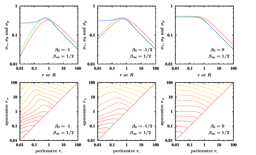
Figure 1: Top. Radial (red), tangential (green) and projected (blue) velocity dispersion profiles for three Plummer models with anisotropy values $\beta_{0}$ and $\beta_{\infty}$ displayed in the figures. Bottom. The distribution function of these models, represented by isoprobability contours in turning point space. High values are indicated by red contours, low values by yellow contours. In all plots, we have used normalized units with $G=M=b=1$.

In the top panels of Fig. 1 we plot the radial and tangential velocity dispersions for a set of anisotropic Plummer models. The three models in this figure all have the same anisotropy $\beta_{\infty}=\tfrac{1}{2}$ at large radii, but a different central anisotropy. Apart from the radial and transversal velocity dispersion, we also plot the projected velocity dispersion $\sigma_{\text{p}}(R)$ on the plane of the sky, defined through

$$\rho_{\text{p}}(R)\,\sigma_{\text{p}}^{2}(R)=2\int_{R}^{\infty}\left[1-\frac{R^{2}}{r^{2}}\,\beta(r)\right]\frac{\rho(r)\,\sigma_{r}^{2}(r)\,r\,{\text{d}}r}{\sqrt{r^{2}-R^{2}}}.$$ (67)

Here, $\rho_{\text{p}}(R)$ is the projected mass density on the plane of the sky,

$$\rho_{\text{p}}(R)=2\int_{R}^{\infty}\frac{\rho(r)\,r\,{\text{d}}r}{\sqrt{r^{2}-R^{2}}}=\frac{M}{\pi}\,\frac{b^{2}}{(b^{2}+R^{2})^{2}}.$$ (68)

The projected velocity dispersion always reaches a finite value in the centre and has an $R^{-1}$ dependence at large radii,

$$\sigma_{\text{p}}^{2}(R)\sim\frac{3\pi}{128}\,\frac{6-5\beta_{\infty}}{3-\beta_{\infty}}\,\frac{GM}{R}.$$ (69)

The distribution function for our set of Plummer models can be written as

$$F({\mathcal{E}},L)=\frac{3}{2(2\pi)^{5/2}}\,\frac{1}{(GMb)^{3/2}}\,\sum_{j=0}^{\infty}(-1)^{j}\,\binom{\beta_{0}}{j}\,\frac{\Gamma(6+2j-2\beta_{\infty})}{\Gamma(\beta_{\infty}-\beta_{0})}\left(\frac{b{\mathcal{E}}}{GM}\right)^{7/2+2j-2\beta_{\infty}}{\mathbb{H}}\left(-\beta_{0},\beta_{\infty},\frac{9}{2}+2j-2\beta_{\infty},1;\frac{L^{2}}{2b^{2}{\mathcal{E}}}\right),$$ (70)

where the function $\mathbb{H}(a,b,c,d;x)$ is a function defined as (Dejonghe 1986)

$$\mathbb{H}(a,b,c,d;x)=G_{2,2}^{1,1}\left(x\left|\,\begin{matrix}1-b,c\\ a,1-d\end{matrix}\,\right.\right)\equiv H_{2,2}^{1,1}\left(x\left|\,\begin{matrix}(1-b,1),(c,1)\\ (a,1),(1-d,1)\end{matrix}\,\right.\right),$$ (71)

with $G^{m,n}_{p,q}(z)$ the Meijer $G$-function. This $\mathbb{H}$-function can conveniently be expressed as

$$\mathbb{H}(a,b,c,d;x)=\begin{cases}\;\dfrac{\Gamma(a+b)}{\Gamma(c-a)\,\Gamma(a+d)}\,x^{a}\,{}_{2}F_{1}(a+b,1+a-c;a+d;x)&\qquad\text{if }x<1,\\[11.38109pt] \;\dfrac{\Gamma(a+b)}{\Gamma(d-b)\,\Gamma(b+c)}\,\left(\dfrac{1}{x}\right)^{b}{}_{2}F_{1}\left(a+b,1+b-d;b+c;\dfrac{1}{x}\right)&\qquad\text{if }x>1.\end{cases}$$ (72)

In the bottom panels of Fig. 1 we plot the distribution function as a contour plot in the turning point space for the same models as the upper panels. The change in anisotropy from tangentially anisotropic at small radii to radially anisotropic at large radii can easily be seen in the slope of these contours.

An interesting subset of models in our two-parameter family of Plummer models is the one-parameter family with $\beta_{0}=0$. These models are isotropic in the inner regions and become anisotropic at large radii. Their augmented density is given by

$$\tilde{\rho}(\psi,r)=\frac{3M}{4\pi\,b^{3}}\left(\frac{b\psi}{GM}\right)^{5-2\beta_{\infty}}\left(1+\frac{r^{2}}{b^{2}}\right)^{-\beta_{\infty}}.$$ (73)

and in the expression for the distribution function (70) only the term corresponding to $j=0$ remains

$$F({\mathcal{E}},L)=\frac{3}{2(2\pi)^{5/2}}\,\frac{1}{(GMb)^{3/2}}\frac{\Gamma(6-2\beta_{\infty})}{\Gamma(\beta_{\infty})}\left(\frac{b{\mathcal{E}}}{GM}\right)^{7/2-2\beta_{\infty}}{\mathbb{H}}\left(0,\beta_{\infty},\frac{9}{2}-2\beta_{\infty},1;\frac{L^{2}}{2b^{2}{\mathcal{E}}}\right).$$ (74)

This subfamily of our current set of Plummer models was already presented by Dejonghe (1987). Most of the kinematical properties, including the projected properties such as dispersions and higher-order moments of the line profiles, can be calculated completely analytically.

5.2 A family of anisotropic Hernquist models

Another extremely popular and simple potential-density pair is the Hernquist model, defined by

$$\psi(r)=\frac{GM}{b+r},$$ (75)

$$\rho(r)=\frac{M}{2\pi}\,\frac{b}{r\left(b+r\right)^{3}}.$$ (76)

Contrary to the Plummer model, this model has a central $r^{-1}$ density cusp and a more realistic $r^{-4}$ behaviour at large radii. We can do the same experiment for the Hernquist model as we did for the Plummer model. If we combine the potential-density pair (75)-(76) with expression (39) and (45), we obtain

$$\frac{M}{2\pi b^{3}}\left(\frac{r}{b}\right)^{-1}\left(1+\frac{r}{b}\right)^{-3}=\rho_{0}\left(1+\frac{r}{b}\right)^{-p}\left[1-\left(1+\frac{r}{b}\right)^{-s}\right]^{q}\left(\frac{r}{r_{\text{a}}}\right)^{-2\beta_{0}}\left(1+\frac{r^{2\delta}}{r_{\text{a}}^{2\delta}}\right)^{-(\beta_{\infty}-\beta_{0})/\delta}.$$ (77)

Similarly as for the Plummer model, it is clear that we will only be able to find a general non-trivial solution if we set

$$s=2\delta=1,$$ (78)

$$r_{\text{a}}=b.$$ (79)

This yields the equation

$$\frac{M}{2\pi b^{3}\rho_{0}}\left(\frac{r}{b}\right)^{-1-q+2\beta_{0}}\left(1+\frac{r}{b}\right)^{-3+p+q+2\beta_{\infty}-2\beta_{0}}=1,$$ (80)

from which we find

$$\rho_{0}=\frac{M}{2\pi b^{3}},$$ (81)

$$p=4-2\beta_{\infty},$$ (82)

$$q=2\beta_{0}-1.$$ (83)

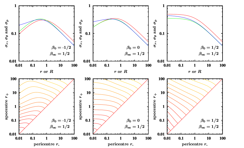
Figure 2: Top. Radial (red), tangential (green) and projected (blue) velocity dispersion profiles for three Hernquist models with anisotropy values $\beta_{0}$ and $\beta_{\infty}$ displayed in the figures. Bottom. The distribution function of these models, represented by isoprobability contours in turning point space. High values are indicated by red contours, low values by yellow contours. In all plots, we have used normalized units with $G=M=b=1$.

We have now defined a two-parameter family of self-consistent Hernquist models with augmented density

$$\tilde{\rho}(\psi,r)=\frac{M}{2\pi b^{3}}\,\left(\frac{b\psi}{GM}\right)^{4-2\beta_{\infty}}\left(1-\frac{b\psi}{GM}\right)^{2\beta_{0}-1}\left(\frac{r}{b}\right)^{-2\beta_{0}}\left(1+\frac{r}{b}\right)^{-2(\beta_{\infty}-\beta_{0})}.$$ (84)

The parameter $\beta_{\infty}$ can assume all values, whereas the central anisotropy $\beta_{0}$ is limited to $\beta_{0}\leqslant\tfrac{1}{2}$, in agreement with the cusp slope-central anisotropy theorem of An & Evans (2006b). By construction, the anisotropy profile of this family of Hernquist models reads

$$\beta(r)=\frac{\beta_{0}b+\beta_{\infty}r}{b+r},$$ (85)

which has the desired behaviour at small and large radii. The radial dispersion profile reads

$$\sigma_{r}^{2}(r)=\frac{GM}{b}\left(\frac{r}{b}\right)^{1-2\beta_{0}}\left(1+\frac{r}{b}\right)^{3-2(\beta_{\infty}-\beta_{0})}B_{\frac{b}{b+r}}(5-2\beta_{\infty},2\beta_{0}).$$ (86)

At large radii, the radial velocity dispersion profile falls as $r^{-1}$,

$$\sigma_{r}^{2}(r)\sim\frac{1}{5-2\beta_{\infty}}\,\frac{GM}{r},$$ (87)

whereas the asymptotic behaviour at small radii is

$$\sigma_{r}^{2}(r)\sim\begin{cases}\;-\dfrac{GM}{b}\,\dfrac{1}{2\beta_{0}}\,\dfrac{r}{b}&\qquad\text{if }\beta_{0}<0,\\[11.38109pt] \;\dfrac{GM}{b}\,B(5-2\beta_{\infty},2\beta_{0})\left(\dfrac{r}{b}\right)^{1-2\beta_{0}}&\qquad\text{if }\beta_{0}>0.\end{cases}$$ (88)

The radial velocity dispersion hence always disappears in the centre, except for the models with the largest allowed central anisotropy ($\beta_{0}=\tfrac{1}{2}$) where it reaches a finite value. For the asymptotic behaviour of the tangential velocity dispersions $\sigma_{\theta}(r)=\sigma_{\varphi}(r)$ at large radii we obtain

$$\sigma_{\theta}^{2}(r)=\sigma_{\varphi}^{2}(r)\sim\frac{1-\beta_{\infty}}{5-2\beta_{\infty}}\,\frac{GM}{r},$$ (89)

whereas at small radii

$$\sigma_{\theta}^{2}(r)=\sigma_{\varphi}^{2}(r)\sim\begin{cases}\;-\dfrac{GM}{b}\,\dfrac{1-\beta_{0}}{2\beta_{0}}\,\dfrac{r}{b}&\qquad\text{if }\beta_{0}<0,\\[11.38109pt] \;\dfrac{GM}{b}\,(1-\beta_{0})\,B(5-2\beta_{\infty},2\beta_{0})\left(\dfrac{r}{b}\right)^{1-2\beta_{0}}&\qquad\text{if }\beta_{0}>0.\end{cases}$$ (90)

The projected velocity dispersion on the plane of the sky has a $R^{-1}$ dependence at large radii,

$$\sigma_{\text{p}}^{2}(R)\sim\frac{8}{15\pi}\,\frac{5-4\beta_{\infty}}{5-2\beta_{\infty}}\,\frac{GM}{R}.$$ (91)

The distribution function can most conveniently be written as a series of hypergeometric functions

$$F({\mathcal{E}},L)=\frac{1}{(2\pi)^{5/2}}\,\frac{1}{(GMb)^{3/2}}\,\left(\frac{b{\mathcal{E}}}{GM}\right)^{5/2-2\beta_{\infty}}\\ \times\sum_{k=0}^{\infty}\binom{{\beta_{\delta}}}{k}\,\frac{\Gamma(5-2\beta_{\infty})}{\Gamma\left(1-\beta_{0}+\frac{k}{2}\right)\Gamma\left(\tfrac{7}{2}-2\beta_{\infty}+\beta_{0}-\frac{k}{2}\right)}\left(\frac{L^{2}}{2b^{2}{\mathcal{E}}}\right)^{-\beta_{0}+k/2}\,{}_{2}F_{1}\left(5-2\beta_{\infty},1-2\beta_{0};\frac{7}{2}-\beta_{\infty}+\frac{k}{2};\frac{b{\mathcal{E}}}{GM}\right)$$ (92)

if $L^{2}<2b^{2}{\mathcal{E}}$, and as

$$F({\mathcal{E}},L)=\frac{1}{(2\pi)^{5/2}}\,\frac{1}{(GMb)^{3/2}}\,\left(\frac{b{\mathcal{E}}}{GM}\right)^{5/2-2\beta_{\infty}}\\ \times\sum_{k=0}^{\infty}\binom{{\beta_{\delta}}}{k}\,\frac{\Gamma(5-2\beta_{\infty})}{\Gamma\left(1-\beta_{\infty}-\frac{k}{2}\right)\Gamma\left(\tfrac{7}{2}-\beta_{\infty}+\frac{k}{2}\right)}\left(\frac{L^{2}}{2b^{2}{\mathcal{E}}}\right)^{-\beta_{\infty}-k/2}\,{}_{2}F_{1}\left(5-2\beta_{\infty},1-2\beta_{0};\frac{7}{2}-2\beta_{\infty}+\beta_{0}-\frac{k}{2};\frac{b{\mathcal{E}}}{GM}\right)$$ (93)

if $L^{2}>2b^{2}{\mathcal{E}}$. These sums only contain a finite number of terms if ${\beta_{\delta}}$ is a positive integer number, i.e. when $(\beta_{0}-\beta_{\infty})$ is a positive integer or half-integer number. This particular subset of models, in which the outer regions are always more tangentially anisotropic than the central regions, has already been discussed by Baes & Dejonghe (2002).

In a similar manner as for the Plummer model, we plot in Fig. 2 the velocity dispersions and the distribution function for three Hernquist models with the same anisotropy $\beta_{\infty}$ but different anisotropy $\beta_{0}$.

5.3 Generalization to a three-parameter family of anisotropic Veltmann models

It is well-known that the Plummer and the Hernquist potential-density pairs can be generalized to a one-parameter family of models characterized by

$$\psi(r)=\frac{GM}{(b^{\lambda}+r^{\lambda})^{1/\lambda}},$$ (94)

$$\rho(r)=\frac{(1+\lambda)\,M}{4\pi}\,\frac{b^{\lambda}}{r^{2-\lambda}\,(b^{\lambda}+r^{\lambda})^{2+1/\lambda}}.$$ (95)

This potential-density pair was first described by Veltmann (1979) and is a special subset (the $\alpha$-models) of the general set of potential-density pairs considered by Zhao (1996). This potential-density pair recently regained much interest because it supports dynamical models that are hypervirial, i.e. in which the virial relation is not only satisfied on a global but also on a local level (Evans & An 2005; Iguchi et al. 2006; Sota et al. 2006). The parameter $\lambda$, lying in the range $0<\lambda\leqslant 2$, determines the slope of the central density cusp. We easily recognize the Plummer model with $\lambda=2$ as the only core-density member of the family and the Hernquist model as the model with $\lambda=1$.

We can now repeat the same exercise as for the Plummer and Hernquist models. After a little bit of algebra, we find that the parameters

$$\rho_{0}=\frac{(1+\lambda)\,M}{4\pi b^{3}},$$ (96)

$$p=3+\lambda-2\beta_{\infty},$$ (97)

$$q=1+\frac{2\left(\beta_{0}-1\right)}{\lambda},$$ (98)

$$s=2\delta=\lambda,$$ (99)

$$r_{\text{a}}=b,$$ (100)

are the general solution for the condition of self-consistency. Notice that the initial condition $q\leqslant 0$ implies $\beta_{0}\leqslant 1-\lambda/2$, which is in correspondence with the cusp slope-central anisotropy theorem (An & Evans 2006b). In other words, for this family the condition $q\leqslant 0$ is also necessary to yield physical models. In this manner we have constructed a three-parameter family of dynamical models defined by the augmented density

$$\tilde{\rho}(\psi,r)=\frac{(1+\lambda)\,M}{4\pi b^{3}}\left(\frac{b\psi}{GM}\right)^{3+\lambda-2\beta_{\infty}}\left[1-\left(\frac{b\psi}{GM}\right)^{\lambda}\right]^{1+2(\beta_{0}-1)/\lambda}\left(\frac{r^{\lambda}}{b^{\lambda}}\right)^{-2\beta_{0}/\lambda}\left(1+\frac{r^{\lambda}}{b^{\lambda}}\right)^{-2(\beta_{\infty}-\beta_{0})/\lambda}.$$ (101)

This augmented density self-consistently supports the one-parameter potential-density pair (94)-(95) and has by construction an anisotropy profile

$$\beta(r)=\frac{\beta_{0}b^{\lambda}+\beta_{\infty}r^{\lambda}}{b^{\lambda}+r^{\lambda}},$$ (102)

which varies smoothly from $\beta_{0}$ in the centre towards $\beta_{\infty}$ at large radii. The radial velocity dispersion can be written as

$$\sigma_{r}^{2}(r)=\frac{GM}{\lambda b}\left(\frac{r^{\lambda}}{b^{\lambda}}\right)^{-1+2(1-\beta_{0})/\lambda}\left(1+\frac{r^{\lambda}}{b^{\lambda}}\right)^{2+(1-2(\beta_{\infty}-\beta_{0}))/\lambda}B_{\frac{b^{\lambda}}{b^{\lambda}+r^{\lambda}}}\left(1+\frac{2\,(2-\beta_{\infty})}{\lambda},2-\frac{2\,(1-\beta_{0})}{\lambda}\right).$$ (103)

For general values of $\lambda$, the distribution function cannot be simplified and should be taken as in formula (41) with the values (96)-(100). For rational values of $\lambda$ however, distribution function simplifies to a sum of generalized hypergeometric functions. One such case is the model with $\lambda=1/2$, for which we obtain the potential-density pair

$$\psi(r)=\frac{GM}{\left(\sqrt{b}+\sqrt{r}\right)^{2}},$$ (104)

$$\rho(r)=\frac{3M}{8\pi}\,\frac{\sqrt{b}}{r^{3/2}\,\left(\sqrt{b}+\sqrt{r}\right)^{4}}.$$ (105)

This model has a central density cups with a slope $\rho(r)\propto r^{-3/2}$, which has been obtained by numerical simulations for dark matter haloes in a CDM cosmological model (Moore et al. 1998).

6 Discussion and conclusions

In this paper, we have described a method to construct self-consistent spherical dynamical models that have an arbitrary density and an arbitrary anisotropy profile. While the general formulation is not so useful since the inversion formulae are rather complicated and numerically unstable, we propose an approach with a parameterized anisotropy profile. We put forward a very general four-parameter anisotropy profile in which the four parameters control the anisotropy at the centre and at large radii, the typical transition radius between the two regimes and the sharpness in which this transition takes place. This parameterized function can therefore represent a large number of monotonically varying anisotropy profiles.

Based on these anisotropy profiles, we present a seven-parameter set of dynamical components that all have the same anisotropy. For each of these components the augmented density $\tilde{\rho}(\psi,r)$ is a sufficiently simple function so that the corresponding distribution function can be written analytically (as a double series). For many reasonable choices of the parameters, the distribution function can be written as a sum of generalized hypergeometric series. The lower-order moments can be expressed by simple analytical functions – for example, the velocity dispersions of all components can be expressed as incomplete Beta functions.

Once the anisotropy profile has been fixed, the construction of a dynamical model with a given potential-density pair consists of a determination of the best linear combination of the various components. This can be achieved with a quadratic programming approach, a technique already in use by various dynamical modellers (Dejonghe 1989; Kuijken & Merrifield 1993; Merrifield & Kuijken 1994; Gerhard et al. 1998). This dynamical modelling technique is rather advanced: dynamical models can be constructed by fitting a variety of data, such as any moments of the distribution function, the projected moments along the line of sight, the full line profiles or even complete spectra. One could argue what the novelty of our approach is compared to the general powerful techniques already presented by these authors. The use of the quadratic programming technique is very general and does not require all components to have the same anisotropy profile. Any possible combination of components can in principle be combined. The main strategy usually consists in choosing the components in such a way that the distribution functions are simple enough; one can for example choose only Fricke components which are double power laws both in augmented density and distribution function. As long as the data base of possible models is large enough, such components allow to fit basically any dynamical model since a linear combination of two components with a different density profile and different constant anisotropy results in a model with a non-constant anisotropy. However, practice has learned that it is generally difficult to construct models with a strong radial anisotropy at large radii. The reason for this problem is that one needs to populate the model with radial orbits that reach large radii. Since such orbits also contribute to the density at small radii, it requires a delicate fine-tuning of the different components to both satisfy the density and anisotropy constraints at small radii while still retaining the radial anisotropy at large radii. In our present case, this problem does not surface since we only have to fit the function $f(\psi)$, or equivalently the density profile. Any combination of the base components will automatically have the correct anisotropy profile. This was actually one of the motivations for the construction of this set of dynamical components.

Apart from presenting an approach to construct detailed dynamical models with a given density and anisotropy profile, our study has also lead to a set of simple one-component dynamical models. The models we have generated are self-consistent realizations of the Plummer and Hernquist models. We have also generalized these models to a complete set of models that self-consistently generate the family of Veltmann (or generalized Plummer) potential-density pairs. Contrary to most analytical dynamical models that have appeared in the literature, the anisotropy profile of these new dynamical models can be chosen arbitrarily in the sense that we can choose the anisotropy at both small and large radii. Both numerical simulations and observational evidence clearly indicates that the outer regions of galaxies and dark matter haloes are typically mildly to significantly radially anisotropic and that the inner regions can be significantly non-isotropic. Realistic simulations should use this information and not impose unrealistic constraints on the anisotropy. We therefore believe that these new analytical models are an important step forward compared to the isotropic or Osipkov-Merritt type dynamical models that are often used. We encourage numerical astrophysicists to use these new distribution functions to generate the initial conditions for their simulations of galaxies or dark matter haloes. Numerical implementation of the most important dynamical properties of these models can be obtained from the authors.

We are currently employing the modelling technique described in this paper to construct dynamical models for dark matter haloes (Van Hese, Baes & Dejonghe 2007). We are using constraints on the density and the anisotropy profile of these haloes from detailed $N$-body simulations. This will be useful to investigate the phase space structure of dynamical models and will also provide the community with an advanced toy model for dark haloes from which more simulations can be initiated. This nicely illustrates that the rise of numerical simulations does not erase the need for analytical work, but rather that there is a symbiosis between both approaches.

Appendix A Derivation of the distribution function

We now present the detailed calculation of the distribution function corresponding with the augmented density (34). We have to consider several cases, depending on the parameter $\beta_{\delta}$.

A.1 Case 1: $\beta_{\delta}$ is a natural number

First, we consider the special case where $\beta_{\delta}$ is zero or a natural number. Then the augmented density is simply a finite sum of positive Fricke components (Fricke 1952; Hénon 1973)

$$\tilde{\rho}(\psi,r)=\rho_{0}\left(\frac{\psi}{\psi_{0}}\right)^{p}\sum_{k=0}^{\beta_{\delta}}\binom{\beta_{\delta}}{k}\left(\frac{r}{r_{\text{a}}}\right)^{-2\beta_{0}+2k\delta},$$ (106)

which leads immediately to equation (36).

A.2 Case 2: $\beta_{\delta}<0$

When $\beta_{\delta}<0$ we can apply the Laplace-Mellin formalism: the connection between the distribution function and the augmented density is then (Dejonghe 1986)

$$\operatorname*{{\mathcal{L}}}_{{\mathcal{E}}\rightarrow\xi}\,\operatorname*{{\mathcal{M}}}_{L\rightarrow\eta}\,\{F({\mathcal{E}},L)\}=\frac{2^{\eta/2}}{M(2\pi)^{3/2}}\frac{\xi^{(3-\eta)/2}}{\Gamma\left(1-\frac{\eta}{2}\right)}\,\operatorname*{{\mathcal{L}}}_{\psi\rightarrow\xi}\,\operatorname*{{\mathcal{M}}}_{r\rightarrow\eta}\,\{\tilde{\rho}(\psi,r)\}.$$ (107)

Since the augmented density is a separable function of $\psi$ and $r$, the transforms can be calculated separately:

$$\operatorname*{{\mathcal{L}}}_{\psi\rightarrow\xi}\,\left\{\psi^{p}\right\}=\int_{0}^{\infty}e^{-\xi\psi}\psi^{p}\,{\text{d}}\psi=\frac{\Gamma(1+p)}{\xi^{1+p}},$$ (108)

and

$$\operatorname*{{\mathcal{M}}}_{r\rightarrow\eta}\,\left\{\left(\frac{r}{r_{\text{a}}}\right)^{-2\beta_{0}}\left(1+\frac{r^{2\delta}}{r_{\text{a}}^{2\delta}}\right)^{\beta_{\delta}}\right\}=\int_{0}^{\infty}r^{\eta-1}\left(\frac{r}{r_{\text{a}}}\right)^{-2\beta_{0}}\left(1+\frac{r^{2\delta}}{r_{\text{a}}^{2\delta}}\right)^{-(\beta_{\infty}-\beta_{0})/\delta}{\text{d}}r=\frac{r_{a}^{\eta}}{2\delta}B\left(\frac{\eta-2\beta_{0}}{2\delta},\frac{2\beta_{\infty}-\eta}{2\delta}\right),$$ (109)

where $\eta$ lies in the convergence strip $2\beta_{0}<\eta<2\beta_{\infty}$. Thus

$$\operatorname*{{\mathcal{L}}}_{{\mathcal{E}}\rightarrow\xi}\,\operatorname*{{\mathcal{M}}}_{L\rightarrow\eta}\,\{F({\mathcal{E}},L)\}=\frac{\rho_{0}2^{\eta/2}}{M\psi_{0}^{p}(2\pi)^{3/2}}\frac{r_{a}^{\eta}}{2\delta}\frac{\Gamma(1+p)}{\Gamma\left(1-\frac{\eta}{2}\right)}B\left(\frac{\eta-2\beta_{0}}{2\delta},\frac{2\beta_{\infty}-\eta}{2\delta}\right)\xi^{(1-\eta)/2-p}.$$ (110)

The inversion of the Laplace transform is straightforward,

$${\operatorname*{{\mathcal{L}}}_{\xi\rightarrow{\mathcal{E}}}}^{-1}\,\left\{\xi^{(1-\eta)/2-p}\right\}=\frac{1}{2\pi i}\int_{\xi_{0}-i\infty}^{\xi_{0}+i\infty}e^{{\mathcal{E}}\xi}\xi^{(1-\eta)/2-p}\,{\text{d}}\xi=\frac{{\mathcal{E}}^{p-(3-\eta)/2}}{\Gamma\left(p-\frac{1-\eta}{2}\right)},$$ (111)

leaving us with the inversion of the Mellin transform

$$F({\mathcal{E}},L) =\frac{\rho_{0}}{M(2\pi\psi_{0})^{3/2}}\frac{\Gamma(1+p)}{\delta\,\Gamma(-\beta_{\delta})}\left(\frac{{\mathcal{E}}}{\psi_{0}}\right)^{p-3/2}{\operatorname*{{\mathcal{M}}}_{\eta\rightarrow L}}^{-1}\,\left\{\frac{1}{2}\frac{\Gamma\left(\frac{\eta-2\beta_{0}}{2\delta}\right)\,\Gamma\left(\frac{2\beta_{\infty}-\eta}{2\delta}\right)}{\Gamma\left(1-\frac{\eta}{2}\right)\,\Gamma\left(p-\frac{1-\eta}{2}\right)}\,\left(2r_{\text{a}}^{2}{\mathcal{E}}\right)^{\eta/2}\right\},$$

$$=\frac{\rho_{0}}{M(2\pi\psi_{0})^{3/2}}\frac{\Gamma(1+p)}{\delta\,\Gamma(-\beta_{\delta})}\left(\frac{{\mathcal{E}}}{\psi_{0}}\right)^{p-3/2}\frac{1}{2\pi i}\int_{C}\frac{\Gamma\left(\frac{s-\beta_{0}}{\delta}\right)\,\Gamma\left(\frac{\beta_{\infty}-s}{\delta}\right)}{\Gamma\left(1-s\vphantom{\frac{1}{1}}\right)\,\Gamma\left(p-\frac{1}{2}+s\right)}\,\left(\frac{L^{2}}{2r_{\text{a}}^{2}{\mathcal{E}}}\right)^{-s}{\text{d}}s.$$ (112)

Taking into account the definition of the Fox $H$-function,

$$H_{p,q}^{m,n}\left(z\left|\,\begin{matrix}\left({\boldsymbol{a}},{\boldsymbol{\alpha}}\right)\\ \left({\boldsymbol{b}},{\boldsymbol{\beta}}\right)\end{matrix}\,\right.\right)=\frac{1}{2\pi i}\int_{\mathcal{C}}\frac{\prod_{j=1}^{m}\Gamma(b_{j}+\beta_{j}s)\,\prod_{j=1}^{n}\Gamma(1-a_{j}-\alpha_{j}s)}{\prod_{j=n+1}^{p}\Gamma(a_{j}+\alpha_{j}s)\,\prod_{j=m+1}^{q}\Gamma(1-b_{j}-\beta_{j}s)}\,z^{-s}\,{\text{d}}s,$$ (113)

the distribution function can be written as

$$F({\mathcal{E}},L)=\frac{\rho_{0}}{M(2\pi\,\psi_{0})^{3/2}}\,\frac{\Gamma(1+p)}{\delta\,\Gamma(-{\beta_{\delta}})}\,\left(\frac{{\mathcal{E}}}{\psi_{0}}\right)^{p-3/2}\,H_{2,2}^{1,1}\left(\frac{L^{2}}{2r_{\text{a}}^{2}{\mathcal{E}}}\left|\,\begin{array}[]{r@{\,,\,}l}\left(1-\frac{\beta_{\infty}}{\delta},\frac{1}{\delta}\right)&\left(p-\frac{1}{2},1\right)\\[5.69054pt] \left(-\frac{\beta_{0}}{\delta},\frac{1}{\delta}\right)&\left(0,1\right)\end{array}\,\right.\right),$$ (114)

or equivalently

$$F({\mathcal{E}},L)=\frac{\rho_{0}}{M(2\pi\,\psi_{0})^{3/2}}\,\frac{\Gamma(1+p)}{\Gamma(-{\beta_{\delta}})}\,\left(\frac{{\mathcal{E}}}{\psi_{0}}\right)^{p-3/2}\,H_{2,2}^{1,1}\left(\left(\frac{L^{2}}{2r_{\text{a}}^{2}{\mathcal{E}}}\right)^{\delta}\left|\,\begin{array}[]{r@{\,,\,}l}\left(1-\frac{\beta_{\infty}}{\delta},1\right)&\left(p-\frac{1}{2},\delta\right)\\[5.69054pt] \left(-\frac{\beta_{0}}{\delta},1\right)&\left(0,\delta\right)\end{array}\,\right.\right).$$ (115)

The integration can be performed along three possible paths $C$, which are equivalent: if the integral converges for more than one of these three paths, then the result is the same. If the integral converges for only one path, then that is the only one to be considered. The valid contours are

• $C$ is a path $C_{1}$ from $-i\infty$ to $i\infty$, such that the poles of $\Gamma\left(\frac{s-\beta_{0}}{\delta}\right)$ lie on one side and the poles of $\Gamma\left(\frac{\beta_{\infty}-s}{\delta}\right)$ lie on the other side. The convergence is absolute if $\delta<1$ or if $\delta=1$ and $p-\frac{1}{2}+\beta_{\delta}>0$. This condition is found by investigating the more familiar criterion for Meijer $G$-functions (see Appendix B). In addition, if $\delta=1$ and $p+\frac{1}{2}+\beta_{\delta}>0$ the integral is semi-convergent for $L^{2}\neq 2r_{\text{a}}^{2}{\mathcal{E}}$ (Dejonghe 1986, Appendix).

• $C$ is a loop $C_{2}$, starting and ending at $-\infty$, that encircles the poles of $\Gamma\left(\frac{s-\beta_{0}}{\delta}\right)$ once in the positive direction and none of the poles of $\Gamma\left(\frac{\beta_{\infty}-s}{\delta}\right)$. The integral then converges if $L^{2}<2r_{\text{a}}^{2}{\mathcal{E}}$.

• $C$ is a loop $C_{3}$, starting and ending at $+\infty$, that encircles the poles of $\Gamma\left(\frac{\beta_{\infty}-s}{\delta}\right)$ once in the negative direction and none of the poles of $\Gamma\left(\frac{s-\beta_{0}}{\delta}\right)$. The integral then converges if $L^{2}>2r_{\text{a}}^{2}{\mathcal{E}}$.

It can easily be seen that the convergence criterion for path $C_{1}$ ensures a well-defined distribution function, i.e. continuous and non-negative. Indeed, in this case the contour is a line parallel to the imaginary axis from $s_{0}-i\infty$ to $s_{0}+i\infty$ with $\beta_{0}<s_{0}<\beta_{\infty}$. On this path the real part of the Gamma functions is positive (where the condition $p+2\beta_{\infty}>3$ ensures that $p-\frac{1}{2}+s>0$ by choosing $s_{0}$ sufficiently close to $\beta_{\infty}$). Hence, the distribution function is non-negative everywhere.

A.3 Case 3: $\beta_{\delta}>0$ and not a natural number

In the case of $\beta_{\delta}>0$ and not a natural number, the Mellin transform does not exist. However, we can solve this problem by rewriting the augmented density in a similar way as equation (106): defining $n$ as the smallest natural number such that $n>\beta_{\delta}$, we obtain

$$\tilde{\rho}(\psi,r)=\rho_{0}\left(\frac{\psi}{\psi_{0}}\right)^{p}\sum_{k=0}^{n}\binom{n}{k}\,\left(\frac{r}{r_{\text{a}}}\right)^{-2\beta_{0}+2k\delta}\left(1+\frac{r^{2\delta}}{r_{\text{a}}^{2\delta}}\right)^{\beta_{\delta}-n}.$$ (116)

For the individual terms the Laplace-Mellin formalism does apply, and the distribution function becomes

$$F({\mathcal{E}},L)=\frac{\rho_{0}}{M(2\pi\psi_{0})^{3/2}}\frac{\Gamma(1+p)}{\delta\,\Gamma(n-\beta_{\delta})}\left(\frac{{\mathcal{E}}}{\psi_{0}}\right)^{p-3/2}\sum_{k=0}^{n}\binom{n}{k}\,\frac{1}{2\pi i}\int_{C_{(k)}}\frac{\Gamma\left(\frac{s-\beta_{0}}{\delta}+k\right)\,\Gamma\left(\frac{\beta_{\infty}-s}{\delta}+n-k\right)}{\Gamma\left(1-s\vphantom{\frac{1}{1}}\right)\,\Gamma\left(p-\frac{1}{2}+s\right)}\,\left(\frac{L^{2}}{2r_{\text{a}}^{2}{\mathcal{E}}}\right)^{-s}{\text{d}}s.$$ (117)

Now, it is easily observed that we can choose the integration paths $C_{(k)}$ to be identical, as the contours $C_{1}$, $C_{2}$ or $C_{3}$ defined above. Therefore the summation can be performed inside the integral. Using the properties

$$\Gamma(x+k)=(x)_{k}\,\Gamma(x)\qquad\mbox{and}\qquad\Gamma(x-k)=(-1)^{k}\frac{\Gamma(x)}{(x)_{k}},$$ (118)

with $(x)_{k}=x(x+1)\cdots(x+k-1)$ the Pochhammer symbol, we find

$$\sum_{k=0}^{n}\binom{n}{k}\,\Gamma\left(\frac{s-\beta_{0}}{\delta}+k\right)\,\Gamma\left(\frac{\beta_{\infty}-s}{\delta}+n-k\right)=\Gamma\left(\frac{s-\beta_{0}}{\delta}\right)\,\Gamma\left(\frac{\beta_{\infty}-s}{\delta}+n\right)\,{}_{2}F_{1}\left(-n,\frac{s-\beta_{0}}{\delta},\frac{s-\beta_{\infty}}{\delta}+1-n;1\right).$$ (119)

Finally, with the identity

$${}_{2}F_{1}(-n,b,c;1)=\frac{(c-b)_{n}}{(c)_{n}},$$ (120)

the equation for the distribution function also reduces to equation (114).

If the convergence criterion for path $C_{1}$ is valid, then every contour $C_{(k)}$ can be taken as a line $s_{k}-i\infty$ to $s_{k}+i\infty$ with $\beta_{0}-k\delta<s_{k}<\beta_{\infty}+(n-k)\delta$. Again, for each $k$ the real part of the integrand is positive, so that the distribution function is well-defined.

Appendix B A practical series expansion for the distribution function

We now seek a more practical form for the distribution function. To this aim we first consider the special case where $\delta$ is a rational number, denoting $\delta=\frac{m}{n}$. Then we can write

$$F({\mathcal{E}},L) =\frac{\rho_{0}}{M(2\pi\psi_{0})^{3/2}}\frac{n\,\Gamma(1+p)}{\Gamma(-\beta_{\delta})}\left(\frac{{\mathcal{E}}}{\psi_{0}}\right)^{p-3/2}\frac{1}{2\pi i}\int_{C}\frac{\Gamma\left(-\frac{n}{m}\beta_{0}+ns\right)\,\Gamma\left(\frac{n}{m}\beta_{\infty}-ns\right)}{\Gamma\left(1-ms\vphantom{\frac{1}{1}}\right)\,\Gamma\left(p-\frac{1}{2}+ms\right)}\left(\frac{L^{2}}{2r_{\text{a}}^{2}{\mathcal{E}}}\right)^{-ms}{\text{d}}s.$$ (121)

Now, using the multiplication formula for the Gamma function

$$\Gamma(kx)=(2\pi)^{(1-k)/2}k^{kx-1/2}\prod_{l=0}^{k-1}\Gamma\left(x+\frac{l}{k}\right),$$ (122)

we can write the integral in the form of a Meijer $G$-function:

$$F({\mathcal{E}},L)=\frac{\rho_{0}}{M(2\pi\psi_{0})^{3/2}}\frac{1}{(2\pi)^{n-m}}\frac{n^{n(\beta_{\infty}-\beta_{0})/m}}{m^{p-1/2}}\frac{\Gamma(1+p)}{\Gamma(-\beta_{\delta})}\left(\frac{{\mathcal{E}}}{\psi_{0}}\right)^{p-3/2}G_{m+n,m+n}^{n,n}\left(\left(\frac{L^{2}}{2r_{\text{a}}^{2}{\mathcal{E}}}\right)^{m}\left|\,\begin{matrix}{\boldsymbol{a}}\\[2.84526pt] {\boldsymbol{b}}\end{matrix}\,\right.\right),$$ (123)

with

$$a_{i} =-\frac{i-1}{n}+\frac{m-\beta_{\infty}}{m} \mbox{for }i=1,\ldots,n,$$

$$a_{n+i} =\hphantom{+}\frac{i-1}{m}+\frac{p-1/2}{m} \mbox{for }i=1,\ldots,m,$$

$$b_{i} =\hphantom{+}\frac{i-1}{n}-\frac{\beta_{0}}{m} \mbox{for }i=1,\ldots,n,$$

$$b_{n+i} =-\frac{i-1}{m}+\frac{m-1}{m} \mbox{for }i=1,\ldots,m.$$ (124)

Since for a general Meijer $G$-function

$$G_{p,q}^{m,n}\left(z\left|\,\begin{matrix}{\boldsymbol{a}}\\[2.84526pt] {\boldsymbol{b}}\end{matrix}\,\right.\right),$$ (125)

with $p=q$ and $z,{\boldsymbol{a}},{\boldsymbol{b}}$ real, the convergence criterion for path $C_{1}$ states that (Mathai 1993)

$$m+n-\frac{1}{2}(p+q)>0$$ (126)

or

$$m+n-\frac{1}{2}(p+q) =0,$$ (127)

$$\sum_{i=0}^{q}b_{i}-\sum_{i=0}^{p}a_{i} <-1,$$ (128)

we indeed obtain the conditions $\delta<1$ or $\delta=1$ and $p-\frac{1}{2}+\beta_{\delta}>0$, as used in Appendix A.

This Meijer $G$-function can be calculated as a sum of generalized hypergeometric functions (Gradshteyn & Ryzhik 1965, eqs. 9.303 and 9.304). For $z<1$ the following equation is valid:

$$G_{m+n,m+n}^{n,n}\left(z^{m}\left|\,\begin{matrix}{\boldsymbol{a}}\\[2.84526pt] {\boldsymbol{b}}\end{matrix}\,\right.\right)= \sum_{i=1}^{n}\frac{\displaystyle\prod_{l=1}^{n}{\vphantom{\prod}}^{\!\prime}\Gamma\,\bigl{(}b_{l}-b_{i}\bigr{)}\prod_{l=1}^{n}\Gamma\,\bigl{(}1+b_{i}-a_{l}\bigr{)}}{\displaystyle\prod_{l=n+1}^{m+n}\Gamma\,\bigl{(}1+b_{i}-b_{l}\bigr{)}\prod_{l=n+1}^{m+n}\Gamma\,\bigl{(}a_{l}-b_{i}\bigr{)}}\,z^{mb_{i}}$$

$$\times \;{}_{m+n}F_{m+n-1}\,\bigl{(}1+b_{i}-a_{1},\ldots,1+b_{i}-a_{m+n}\,;\,\bigr{.}$$

$$\hphantom{\;{}_{m+n}F_{m+n-1}\,\bigl{(}}\bigl{.}1+b_{i}-b_{1},\ldots,*,\ldots,1+b_{i}-b_{m+n}\,;\,(-1)^{m+n}z^{m}\,\bigr{)}\,,$$ (129)

where the prime by the product symbol denotes the omission of the product when $i=l$, and the asterisk in the hypergeometric function indicates the omission on the $i\,$th parameter. Analogously, the equation for $z>1$ reads

$$G_{m+n,m+n}^{n,n}\left(z^{m}\left|\,\begin{matrix}{\boldsymbol{a}}\\[2.84526pt] {\boldsymbol{b}}\end{matrix}\,\right.\right)= \sum_{i=1}^{n}\frac{\displaystyle\prod_{l=1}^{n}{\vphantom{\prod}}^{\!\prime}\Gamma\,\bigl{(}a_{i}-a_{l}\bigr{)}\prod_{l=1}^{n}\Gamma\,\bigl{(}1+b_{l}-a_{i}\bigr{)}}{\displaystyle\prod_{l=n+1}^{m+n}\Gamma\,\bigl{(}1+a_{l}-a_{i}\bigr{)}\prod_{l=n+1}^{m+n}\Gamma\,\bigl{(}a_{i}-b_{l}\bigr{)}}\,z^{m(a_{i}-1)}$$

$$\times \;{}_{m+n}F_{m+n-1}\,\bigl{(}1+b_{1}-a_{i},\ldots,1+b_{m+n}-a_{i}\,;\,\bigr{.}$$

$$\hphantom{\;{}_{m+n}F_{m+n-1}\,\bigl{(}}\bigl{.}1+a_{1}-a_{i},\ldots,*,\ldots,1+a_{m+n}-a_{i}\,;\,(-1)^{m+n}z^{-m}\,\bigr{)}\,.$$ (130)

With the coefficients from equation (124), we obtain for $L^{2}<2r_{\text{a}}^{2}{\mathcal{E}}$

$$G_{m+n,m+n}^{n,n}\left(\left(\frac{L^{2}}{2r_{\text{a}}^{2}{\mathcal{E}}}\right)^{m}\left|\,\begin{matrix}{\boldsymbol{a}}\\[2.84526pt] {\boldsymbol{b}}\end{matrix}\,\right.\right)= \sum_{i=0}^{n-1}\frac{\displaystyle\prod_{l=0}^{n-1}{\vphantom{\prod}}^{\!\prime}\Gamma\left(\frac{l-i}{n}\right)\,\prod_{l=0}^{n-1}\Gamma\left(\frac{\beta_{\infty}-\beta_{0}}{m}+\frac{l+i}{n}\right)}{\displaystyle\prod_{l=0}^{m-1}\Gamma\left(\frac{1-\beta_{0}+l}{m}+\frac{i}{n}\right)\,\prod_{l=0}^{m-1}\Gamma\left(\frac{p+\beta_{0}-1/2+l}{m}-\frac{i}{n}\right)}$$

$$\times \sum_{j=0}^{\infty}\frac{\displaystyle\prod_{l=0}^{n-1}\left(\frac{\beta_{\infty}-\beta_{0}}{m}+\frac{l+i}{n}\right)_{j}\,\prod_{l=0}^{m-1}\left(1-\frac{p+\beta_{0}-1/2+l}{m}+\frac{i}{n}\right)_{j}}{\displaystyle\prod_{l=0}^{n-1}\left(1-\frac{l-i}{n}\right)_{j}\,\prod_{l=0}^{m-1}\left(\frac{1-\beta_{0}+l}{m}+\frac{i}{n}\right)_{j}}(-1)^{(m+n)j}\left(\frac{L^{2}}{2r_{\text{a}}^{2}{\mathcal{E}}}\right)^{-\beta_{0}+i\delta+mj}.$$ (131)

Now, with the aid of the identities

$$\Gamma(x)\,\Gamma(1-x)=\frac{\pi}{\sin(\pi x)},$$ (132)

and

$$\prod_{k=1}^{n-1}\sin\left(\frac{k\pi}{n}\right)=\frac{n}{2^{n-1}},$$ (133)

we can simplify this expression to

$$G_{m+n,m+n}^{n,n}\left(\left(\frac{L^{2}}{2r_{\text{a}}^{2}{\mathcal{E}}}\right)^{m}\left|\,\begin{matrix}{\boldsymbol{a}}\\[2.84526pt] {\boldsymbol{b}}\end{matrix}\,\right.\right)= \sum_{i=0}^{n-1}\sum_{j=0}^{\infty}\frac{\displaystyle\prod_{l=0}^{n-1}\Gamma\left(\frac{\beta_{\infty}-\beta_{0}}{m}+\frac{l+i}{n}+j\right)}{\displaystyle\prod_{l=0}^{n-1}\Gamma\left(\frac{1+l+i}{n}+j\right)\,\prod_{l=0}^{m-1}\Gamma\left(\frac{1-\beta_{0}+l}{m}+\frac{i}{n}+j\right)\,\prod_{l=0}^{m-1}\Gamma\left(\frac{p+\beta_{0}-1/2+l}{m}-\frac{i}{n}-j\right)}$$

$$\times \frac{(2\pi)^{n-1}}{n}(-1)^{i+nj}\left(\frac{L^{2}}{2r_{\text{a}}^{2}{\mathcal{E}}}\right)^{-\beta_{0}+i\delta+mj},$$ (134)

so that, using again equation (122), the distribution function reduces to

$$F({\mathcal{E}},L)= \frac{\rho_{0}}{M(2\pi\psi_{0})^{3/2}}\frac{\Gamma(1+p)}{\Gamma(-\beta_{\delta})}\left(\frac{{\mathcal{E}}}{\psi_{0}}\right)^{p-3/2}$$

$$\times \sum_{i=0}^{n-1}\sum_{j=0}^{\infty}\frac{\Gamma\left(\frac{\beta_{\infty}-\beta_{0}}{\delta}+i+jn\right)}{\Gamma\left(1+i+jn\right)\,\Gamma\left(1-\beta_{0}+i\delta+jm\right)\,\Gamma\left(p+\beta_{0}-1/2-i\delta-jm\right)}(-1)^{i+nj}\left(\frac{L^{2}}{2r_{\text{a}}^{2}{\mathcal{E}}}\right)^{-\beta_{0}+i\delta+mj}.$$ (135)

Finally, the double summation can be grouped into a single index $k=i+nj$, and we obtain for $L^{2}<2r_{\text{a}}^{2}{\mathcal{E}}$

$$F({\mathcal{E}},L)=\frac{\rho_{0}}{M(2\pi\psi_{0})^{3/2}}\left(\frac{{\mathcal{E}}}{\psi_{0}}\right)^{p-3/2}\sum_{k=0}^{\infty}\binom{\beta_{\delta}}{k}\frac{\Gamma(1+p)}{\Gamma(1-\beta_{0}+k\delta)\,\Gamma(p+\beta_{0}-1/2-k\delta)}\left(\frac{L^{2}}{2r_{\text{a}}^{2}{\mathcal{E}}}\right)^{-\beta_{0}+k\delta}.$$ (136)

Similarly, for $L^{2}>2r_{\text{a}}^{2}{\mathcal{E}}$, we find

$$F({\mathcal{E}},L)=\frac{\rho_{0}}{M(2\pi\psi_{0})^{3/2}}\left(\frac{{\mathcal{E}}}{\psi_{0}}\right)^{p-3/2}\sum_{k=0}^{\infty}\binom{\beta_{\delta}}{k}\frac{\Gamma(1+p)}{\Gamma(1-\beta_{\infty}-k\delta)\,\Gamma(p+\beta_{\infty}-1/2+k\delta)}\left(\frac{L^{2}}{2r_{\text{a}}^{2}{\mathcal{E}}}\right)^{-\beta_{\infty}-k\delta}.$$ (137)

Although these expressions have been derived for rational values of $\delta$, they can be generalized to any real value, since these functions are continuous in $\delta$. Hence we indeed obtain equation (36).

References

• An & Evans (2006a) An, J. H., & Evans, N. W. 2006a, AJ, 131, 782
• An & Evans (2006b) An, J. H., & Evans, N. W. 2006b, ApJ, 642, 752
• Baes & Dejonghe (2002) Baes, M., & Dejonghe, H. 2002, A&A, 393, 485
• Baes & Dejonghe (2004) Baes, M., & Dejonghe, H. 2004, MNRAS, 351, 18
• Baes et al. (2005) Baes, M., Dejonghe, H., & Buyle, P. 2005, A&A, 432, 411
• Buyle et al. (2007) Buyle, P., Hunter, C., & Dejonghe, H. 2007, MNRAS, 375, 773
• Carlberg et al. (1997) Carlberg, R. G., et al. 1997, ApJ, 485, L13
• Cole & Lacey (1996) Cole, S., & Lacey, C. 1996, MNRAS, 281, 716
• Colín et al. (2000) Colín, P., Klypin, A. A., & Kravtsov, A. V. 2000, ApJ, 539, 561
• Cuddeford (1991) Cuddeford, P. 1991, MNRAS, 253, 414
• Cuddeford & Louis (1995) Cuddeford, P., & Louis, P. 1995, MNRAS, 275, 1017
• Dehnen (1993) Dehnen, W. 1993, MNRAS, 265, 250
• Dehnen & McLaughlin (2005) Dehnen, W., & McLaughlin, D. E. 2005, MNRAS, 363, 1057
• Dejonghe (1986) Dejonghe, H. 1986, Phys. Rep., 133, 217
• Dejonghe (1987) Dejonghe, H. 1987, MNRAS, 224, 13
• Dejonghe (1989) Dejonghe, H. 1989, ApJ, 343, 113
• Diemand et al. (2004) Diemand, J., Moore, B., & Stadel, J. 2004, MNRAS, 352, 535
• Evans & An (2005) Evans, N. W., & An, J. 2005, MNRAS, 360, 492
• Fricke (1952) Fricke, W. 1952, Astronomische Nachrichten, 280, 193
• Gebhardt et al. (2003) Gebhardt, K., et al. 2003, ApJ, 583, 92
• Gerhard et al. (1998) Gerhard, O., Jeske, G., Saglia, R. P., & Bender, R. 1998, MNRAS, 295, 197
• Gradshteyn & Ryzhik (1965) Gradshteyn, I. S. & Ryzhik, I. M. 1965, Table of integrals, series and products (New York: Academic Press, 1965, 4th ed., edited by Geronimus, Yu.V. (4th ed.); Tseytlin, M.Yu. (4th ed.))
• Fukushige & Makino (2001) Fukushige, T., & Makino, J. 2001, ApJ, 557, 533
• Hansen & Moore (2006) Hansen, S. H., & Moore, B. 2006, New Astronomy, 11, 333
• Hansen & Stadel (2006) Hansen, S. H., & Stadel, J. 2006, Journal of Cosmology and Astro-Particle Physics, 5, 14
• Hénon (1960) Hénon, M. 1960, Annales d’Astrophysique, 23, 474
• Hénon (1973) Hénon, M. 1973, A&A, 24, 229
• Hernquist (1990) Hernquist, L. 1990, ApJ, 356, 359
• Hiotelis (1994) Hiotelis, N. 1994, A&A, 283, 783
• Iguchi et al. (2006) Iguchi, O., Sota, Y., Nakamichi, A., & Morikawa, M. 2006, Phys. Rev. E, 73, 046112
• Kuijken & Merrifield (1993) Kuijken, K., & Merrifield, M. R. 1993, MNRAS, 264, 712
• Jaffe (1983) Jaffe, W. 1983, MNRAS, 202, 995
• Kazantzidis et al. (2004) Kazantzidis, S., Magorrian, J., & Moore, B. 2004, ApJ, 601, 37
• Kronawitter et al. (2000) Kronawitter, A., Saglia, R. P., Gerhard, O., & Bender, R. 2000, A&AS, 144, 53
• Louis (1993) Louis, P. D. 1993, MNRAS, 261, 283
• Mathai (1993) Mathai, A. M. 1993, A Handbook of Generalized Special Functions for Statistical and Physical Sciences, Oxford University Press, Oxford.
• Merrifield & Kuijken (1994) Merrifield, M. R., & Kuijken, K. 1994, ApJ, 432, 575
• Merritt (1985) Merritt, D. 1985, AJ, 90, 1027
• Merritt (1985) Merritt, D. 1985, MNRAS, 214, 25P
• Moore et al. (1998) Moore, B., Governato, F., Quinn, T., Stadel, J., & Lake, G. 1998, ApJ, 499, L5
• Oñorbe et al. (2007) Oñorbe, J., Domínguez-Tenreiro, R., Sáiz, A., & Serna, A. 2007, MNRAS, 376, 39
• Osipkov (1979) Osipkov, L. P. 1979, Pis ma Astronomicheskii Zhurnal, 5, 77
• Plummer (1911) Plummer, H. C. 1911, MNRAS, 71, 460
• Quinlan et al. (1995) Quinlan, G. D., Hernquist, L., & Sigurdsson, S. 1995, ApJ, 440, 554
• Quinlan & Hernquist (1997) Quinlan, G. D., & Hernquist, L. 1997, New Astronomy, 2, 533
• Sota et al. (2006) Sota, Y., Iguchi, O., Morikawa, M., & Nakamichi, A. 2006, Progress of Theoretical Physics Supplement, 162, 62
• Tremaine et al. (1994) Tremaine, S., Richstone, D. O., Byun, Y.-I., Dressler, A., Faber, S. M., Grillmair, C., Kormendy, J., & Lauer, T. R. 1994, AJ, 107, 634
• Van Hese, Baes & Dejonghe (2007) Van Hese, E., Baes, M., & Dejonghe, H. 2007, in preparation
• Veltmann (1979) Veltmann, U. I. K. 1979, AZh, 56, 976
• Zhao (1996) Zhao, H. 1996, MNRAS, 278, 488