Analogue of cosmological particle creation in an ion trap

Abstract

We study phonons in a dynamical chain of ions confined by a trap with a time-dependent (axial) potential strength and demonstrate that they behave in the same way as quantum fields in an expanding/contracting universe. Based on this analogy, we present a scheme for the detection of the analogue of cosmological particle creation which should be feasible with present-day technology. In order to test the quantum nature of the particle creation mechanism and to distinguish it from classical effects such as heating, we propose to measure the two-phonon amplitude via the $2^{\rm nd}$ red side-band and to compare it with the one-phonon amplitude ($1^{\rm st}$ red side-band).

Introduction The theory of quantum fields in curved space-times (see, e.g., birrell ) comprises many fascinating and striking phenomena – one of them being the creation of real particles out of the (virtual) quantum vacuum fluctuations by a gravitational field. These effects include Hawking radiation given off by black holes as well as cosmological particle creation. A very similar mechanism – the amplification of quantum vacuum fluctuations due to the rapid expansion of the very early universe – is (according to our standard model of cosmology) responsible for the generation of the seeds for cosmic structure formation. Hence, even though these effects are far removed from every-day experience, they are very important for the past and the future fate of our universe.

Therefore, it would be desirable to render these phenomena accessible to an experimental verification. Probably the most promising way for achieving this goal is to construct a suitable analogue which reproduces the relevant features (such as the Hamiltonian) of quantum fields in curved space-times. Along this line of reasoning, proposals based on the analogy between phonons in dynamical Bose-Einstein condensates and quantized fields in an expanding/contracting universe have been suggested living . Unfortunately, the detection of the created phonons in these systems is rather difficult (see, however, detect ).

On the other hand, the detection of single phonons in ion traps via optical techniques is already state of the art in current technology – which suggests the study of this set-up instead. In this Letter, we shall derive the analogy between phonons in an axially time-dependent ion trap and quantum fields in an expanding/contracting universe and propose a corresponding detection scheme for the analogue of cosmological particle creation. A similar idea has already been pursued in alsing , but the proposal presented therein goes along with several problems, which will be discussed below kritik .

Cosmological particle creation Let us start by briefly reviewing the basic mechanism of particle creation in an expanding/contracting universe. For simplicity, we consider a massless scalar field $\phi$ described by the action, see, e.g., birrell ($\hbar=c=1$ throughout)

$${\cal A}=\frac{1}{2}\int d^{4}x\,\sqrt{|{\mathfrak{g}}|}\left[(\partial_{\mu}\phi){\mathfrak{g}}^{\mu\nu}(\partial_{\nu}\phi)-\zeta{\mathfrak{R}}\phi^{2}\right]\,,$$ (1)

where ${\mathfrak{g}}^{\mu\nu}$ denotes the metric and ${\mathfrak{g}}={\rm det}\{{\mathfrak{g}}_{\mu\nu}\}$ its determinant. Furthermore, a scalar field can be coupled to the Ricci (curvature) scalar ${\mathfrak{R}}$ via a dimensionless parameter $\zeta$ (e.g., conformal coupling $\zeta=1/6$, cf. birrell ). A spatially flat universe can be described in terms of the Friedman-Robertson-Walker metric

$$ds^{2}={\mathfrak{a}}^{6}(t)dt^{2}-{\mathfrak{a}}^{2}(t)d\mbox{\boldmath$r$}^{2}\,,$$ (2)

with the time-dependent scale parameter ${\mathfrak{a}}(t)$ corresponding to the cosmic expansion/contraction. Here we have chosen a slightly unusual time-coordinate $t$ related to the proper time $\tau$ via $d\tau={\mathfrak{a}}^{3}(t)dt$ in order to simplify the subsequent formulæ. After a normal-mode expansion, the wave equation reads

$$\ddot{\phi}_{\mbox{\boldmath$\scriptstyle k$}}+\left[{\mathfrak{a}}^{4}(t)\mbox{\boldmath$k$}^{2}+\zeta{\mathfrak{a}}^{6}(t){\mathfrak{R}}(t)\right]\phi_{\mbox{\boldmath$\scriptstyle k$}}=0\,,$$ (3)

i.e., each mode $k$ just represents a harmonic oscillator with a time-dependent potential ${\mathfrak{a}}^{4}(t)\mbox{\boldmath$k$}^{2}+\zeta{\mathfrak{a}}^{6}(t){\mathfrak{R}}(t)$. As long as this external time-dependence of the potential is much slower than the internal frequency of the oscillator, the quantum state will stay near the ground state due to the adiabatic theorem. However, if the external time-dependence is fast enough (i.e., non-adiabatic), the evolution will transform the initial ground state into an excited state in general – which is the basic mechanism of cosmological particle creation. In this case, the initial vacuum state $\left|0\right>=\left|\psi(t\downarrow-\infty)\right>$ containing no particles $\forall_{\mbox{\boldmath$\scriptstyle k$}}\,\hat{a}_{\mbox{\boldmath$\scriptstyle k$}}\left|0\right>=0$ evolves into a squeezed state

$$\left|\psi(t\uparrow\infty)\right> = \exp\left\{\sum\limits_{\mbox{\boldmath$\scriptstyle k$}}\xi_{k}\,\hat{a}_{\mbox{\boldmath$\scriptstyle k$}}^{\dagger}\,\hat{a}_{-\mbox{\boldmath$\scriptstyle k$}}^{\dagger}-{\rm h.c.}\right\}\left|0\right>$$ (4)

$$= \left|0\right>+\sum\limits_{\mbox{\boldmath$\scriptstyle k$}}\xi_{k}\left|1_{\mbox{\boldmath$\scriptstyle k$}},1_{-\mbox{\boldmath$\scriptstyle k$}}\right>+{\cal O}(\xi_{k}^{2})\,,$$

which does contain pairs of particles $\left|1_{\mbox{\boldmath$\scriptstyle k$}},1_{-\mbox{\boldmath$\scriptstyle k$}}\right>$. The squeezing parameter $\xi_{k}$ for each mode is determined by the solution of Eq. (3) and thus by the time-dependence of ${\mathfrak{a}}^{4}(t)\mbox{\boldmath$k$}^{2}$ as well as $\zeta{\mathfrak{a}}^{6}(t){\mathfrak{R}}(t)$ and governs the number of created particles per mode

$$\langle\hat{n}_{\mbox{\boldmath$\scriptstyle k$}}\rangle=\left<\psi(t\uparrow\infty)\right|\hat{a}^{\dagger}_{\mbox{\boldmath$\scriptstyle k$}}\hat{a}_{\mbox{\boldmath$\scriptstyle k$}}\left|\psi(t\uparrow\infty)\right>=\sinh^{2}(|\xi_{k}|)\,.$$ (5)

Ion-trap analogue Assuming a strong radial confinement of the ions, we consider their axial motion only. In a time-dependent harmonic axial potential described by the oscillator frequency $\omega_{\rm ax}(t)$, the position $q_{i}$ of the $i$-th ion obeys the equation of motion

$$\ddot{q}_{i}+\omega_{\rm ax}^{2}(t)q_{i}=\gamma\sum\limits_{j\neq i}\frac{{\rm sign}(i-j)}{(q_{i}-q_{j})^{2}}\,,$$ (6)

where the factor $\gamma$ encodes the strength of the Coulomb repulsion between the ions. Assuming a static situation initially, the classical solution to the above equation can be obtained via the scaling ansatz $q_{i}(t)=b(t)q_{i}^{0}$, where $q_{i}^{0}$ are the initial static equilibrium positions, leading to the evolution equation for the scale parameter $b(t)$

$$\ddot{b}+\omega_{\rm ax}^{2}(t)b=\frac{\omega_{\rm ax}^{2}(0)}{b^{2}}\,.$$ (7)

In order to treat the quantum fluctuations of the ions (leading to the quantized phonon modes), let us split the full position operator $\hat{q}_{i}(t)$ for each ion into its classical trajectory $b(t)q_{i}^{0}$ and quantum fluctuations $\delta\hat{q}_{i}(t)$

$$\hat{q}_{i}(t)=b(t)q_{i}^{0}+\delta\hat{q}_{i}(t)\,.$$ (8)

Since these fluctuations $\delta\hat{q}_{i}(t)$ are very small for heavy ions, we may linearize the full equation of motion (6)

$$\left(\frac{\partial^{2}}{\partial t^{2}}+\omega_{\rm ax}^{2}(t)\right)\delta\hat{q}_{i}=\frac{1}{b^{3}(t)}\sum\limits_{j}M_{ij}\delta\hat{q}_{j}\,,$$ (9)

with a time-independent matrix $M_{ij}$ arising from the Coulomb term in (6). Diagonalization of this matrix (normal-mode expansion) yields the phonon modes

$$\left(\frac{\partial^{2}}{\partial t^{2}}+\omega_{\rm ax}^{2}(t)+\frac{\omega_{\kappa}^{2}}{b^{3}(t)}\right)\delta\hat{q}_{\kappa}=0\,,$$ (10)

labeled by $\kappa$. The time-independent eigenvalues $\omega_{\kappa}^{2}\geq 0$ of the matrix $M_{ij}$ determine the phonon frequencies. The lowest mode is the center-of-mass mode corresponding to a simultaneous (rigid) motion of the ions. Since the ion distances are fixed, the Coulomb term does not contribute in this situation $\omega_{\kappa}^{2}=0$. The next mode is the breathing mode with $\omega_{\kappa}^{2}=2\omega_{\rm ax}^{2}(0)$. Comparing Eqs. (7) and (10), we see that this mode exactly corresponds to the scaling ansatz, i.e., the ion cloud expands/contracts linearly. Hence this is the only mode which can be excited classically (for a purely harmonic potential). I.e., without imperfections such as heating, phonons in the other modes can only be created by quantum effects.

Comparing Eqs. (3) and (10) and identifying $\phi_{\mbox{\boldmath$\scriptstyle k$}}$ with $\delta\hat{q}_{\kappa}$, we observe a strong similarity: The wavenumber $\mbox{\boldmath$k$}^{2}$ in  (3) directly corresponds to $\omega_{\kappa}^{2}$ in (10) and the scale factors ${\mathfrak{a}}(t)$ and $b(t)$ enter in a similar way. However, an expanding universe is analogous to a contracting ion cloud and vice versa. In the mode-independent terms, the axial trap frequency $\omega_{\rm ax}$ acts like the Ricci scalar ${\mathfrak{R}}$. Interestingly, both are related to the second time-derivatives of the corresponding scale factors.

In view of the formal equivalence of Eqs. (7) and (10), we obtain the same effects as in cosmology – in particular, the mixing of creation and annihilation operators

$$\hat{a}_{\kappa}(t\uparrow\infty)=\alpha_{\kappa}\hat{a}_{\kappa}(0)+\beta_{\kappa}\hat{a}_{\kappa}^{\dagger}(0)\,,$$ (11)

which can be expressed in terms of the Bogolubov coefficients satisfying $|\alpha_{\kappa}^{2}|-|\beta_{\kappa}^{2}|=1$. Note that the above relation is just the operator representation of the squeezing transformation in Eq. (4) with $|\beta_{\kappa}|\leftrightarrow\sinh(|\xi_{k}|)$.

Detection scheme In the following we describe how to realize the proposed experiment by applying operations closely related to those implemented on qubit-ions in quantum information processing bible98 . We focus on initializing the system, simulating the non-adiabatic expansion of space, performing the read-out of the final state (particle- or phonon-number distribution) and distinguishing it from a classically describable outcome, for example caused by thermal heating. To perform a first realization, we will confine one single earth alkaline atomic ion to the axis of a linear radio-frequency trap pqe07 similar to that described in rowe02 ; ferdi03 . The required simulation basis can be composed by a ²S_1/2 electronic ground state level of ²⁵Mg⁺, here the state $|F=3;m_{f}=3\rangle=\left|\downarrow\right>$, and the associated harmonic oscillator levels $|n\rangle$ related to the axial harmonic confinement, as depicted in Fig. 1. At the start of each experiment, the ion will be laser cooled close to the ground state of the axial (external) motion and optically pumped into the electronic (internal) state $\left|\downarrow\right>$ initial98 . Then we will decrease adiabatically the axial confinement and subsequently reset it non-adiabatically to its initial value (as already proposed in heinz90 in another context). Since the ground state wave function of the ion cannot adapt to the restored stiff confinement (non-adiabatic case), it will oscillate symmetrically around the minimum of the final trapping potential didihabil03 , i.e., without populating odd motional states. As shown above, this non-classical oscillation is to be described via a squeezed state (see also motion96 ) depicted in Fig. 2.

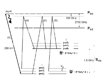
Figure 1: Schematic of the relevant energy levels (not to scale) of one ²⁵Mg⁺ ion. Shown are the ground-state hyperfine levels supplying the two internal states ($\left|\downarrow\right>$ and $\left|\uparrow\right>$) and the first three equidistant harmonic oscillator levels $\left|n\right>$, related to the harmonic axial confinement in a linear ion trap. Typically, the energy splitting of the motional levels and the Zeeman shift induced by an external magnetic field are of the same order of magnitude within 1-10 MHz, therefore much smaller than the Hyperfine splitting of 1.8 GHz, the fine structure splitting of 2750 GHz and the optical transition frequency of the order of $10^{15}$Hz. We depict the resonant transition state sensitive detection named (d) and the relevant types of off- resonant ($\approx$ 100 GHz) two-photon stimulated Raman transitions (a,b and c) described in the text.

We propose, in addition to established schemes described in motion96 or enrique05 , for example, an alternative method to distinguish classical noise (such as the initial thermal distribution or heating during the process) from a squeezed state generated by quantum effects considered here. In order to read out the final motional state, we will first couple it (via suitable lasers) to two internal states of the ion. Besides the electronic ground state $|F=3;m_{f}=3\rangle=\left|\downarrow\right>$, the second internal state to span a two-level system (analogous to a qubit) is implemented via a second hyperfine state of ²⁵Mg⁺, $|F=2,m_{f}=2\rangle\equiv\left|\uparrow\right>$, separated from the state $\left|\downarrow\right>$ by the hyperfine splitting $\omega_{\mathrm{o}}\simeq 2\pi\times 1.8$ GHz. We will accomplish the coupling of the two internal states $\left|\downarrow\right>$, $\left|\uparrow\right>$ and the motional states $|n\rangle$ via two-photon stimulated Raman transitions bible98 requiring two laser beams ($\lambda\approx 280$ nm), with wave vector difference $\Delta\mbox{\boldmath$k$}=\mbox{\boldmath$k_{2}$}-\mbox{\boldmath$k_{1}$}$ aligned along the trap axis $z$ ($|\Delta k|=\sqrt{2}\times 2\pi/\lambda=2\pi/\lambda_{\mathrm{eff}}$). Via detuning the frequency difference $\omega_{2}-\omega_{1}$ from the hyperfine splitting $\omega_{\mathrm{o}}\pm 2\pi m\nu_{z}$ by integer multiples $m$ of the axial trapping frequency $\nu_{z}$, we may drive the carrier-transition ($m=0$) or the first- ($m=1$) and second-($m=2$) sideband transitions respectively. Note that the spectral resolution of the two-photon stimulated Raman transition is independent on the natural line width $\Gamma=2\pi\times$43 MHz of the resonant transition – but proportional to the inverse of the Rabi-frequency, adjusted via the intensities or detuning of the laser beams allowing for the resolution of the individual motional states separated by $\nu_{z}\ll\Gamma$. In order to measure the population of the motional state $|n=2\rangle$, we will drive a sequence of transitions (cf. Fig. 1), synthesized by a second-sideband (a) transition ($\left|\downarrow,n=2\right>\rightarrow\left|\uparrow,n=0\right>$) followed by a carrier (c) transition ($\left|\uparrow,n=0\right>\rightarrow\left|\downarrow,n=0\right>$). The final read-out (d) described below is internal-state dependant and provides us with the population in state $\left|\downarrow\right>$. After the sequence (a,c,d) of transitions this is almost exclusively equivalent to the population of the motional state $|n=2\rangle$ (because the probability of even higher excitations $|n\geq 3\rangle$ is expected to be much smaller and their Rabi frequencies are also different). This result can then be compared with the outcome after a first red-sideband (b) transition ($\left|\downarrow,n=1\right>\rightarrow\left|\uparrow,n=0\right>$) followed by a carrier (c) transition ($\left|\uparrow,n=0\right>\rightarrow\left|\downarrow,n=0\right>$), providing the probability of motional excitation $|n=1\rangle$. As soon as we deduce a higher probability for motional state $|n=2\rangle$ than for motional state $|n=1\rangle$, we show the incompatibility with classical effects such as a thermal distribution and get strong evidence for the non-classical effect of squeezing cohstate .

Finally, we have to read out the internal state efficiently. To this end, we apply an additional resonant laser beam (d), tuned to a cycling transition bible98 , coupling only state $\left|\downarrow\right>$ resonantly to the $P_{3/2}$ level and providing spontaneous emission at rates of $>$ 10 MHz. This allows to distinguish the “bright” $\left|\downarrow\right>$ from the “dark” $\left|\uparrow\right>$ state with high accuracy, even at a low detection efficiency (due to the restricted solid angle etc.).

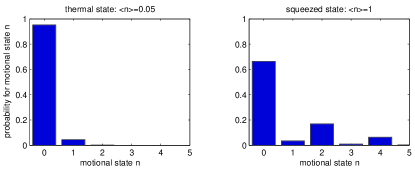
Figure 2: Population of the motional states: On the left hand side, we show the experimentally realized thermal spectrum after cooling the system close to the ground state ($\langle\hat{n}\rangle$=0.05). On the right hand side, we show the simulated spectrum of the ($\langle\hat{n}\rangle$=1) squeezed state, assuming the starting distribution from the left. The almost complete absence of population in odd motional states emphasizes the non-classical character of this state and guides towards a simple possibility to distinguish it from thermal and disturbed ones via measuring a much higher population in state $|n=2\rangle$ than $|n=1\rangle$.

Envisioned results The above mentioned sate of the art techniques allow to cool the axial motion close to the ground state $\langle\hat{n}\rangle\approx 0.05$ pqe07 (see also initial98 ; ferdi03 ) and to optically pump into the down state $\left|\downarrow\right>$ with 99$\%$ pqe07 or even higher fidelity initial98 ; ferdi03 . First experiments show a possible non-adiabatic variation of the axial motional frequency $\nu_{z}$ between 200 kHz and $\geq$ 2 MHz with a related rise time of the order of one micro-second, which is sufficiently fast compared to the oscillation period of the lower frequency. Numerical simulations (based on measured temporal variation curves) indicate that we should be able to transfer approximately 20$\%$ of the motional state population from the ground state $|n=0\rangle$ into state $|n=2\rangle$, which corresponds to a squeezed state with $\langle\hat{n}\rangle\approx 1$. Starting with a thermal distribution with $\langle\hat{n}\rangle\approx 0.05$ instead of the exact ground state $|n=0\rangle$, there will also be a small final population (a few percent) of the state $|n=1\rangle$, see Fig. 2. However, this residual effect will be significantly smaller than the $|n=2\rangle$ population such that the signatures of squeezing can be measured as described above.

Conclusions Since the state of the art fidelities for the carrier and sideband transitions as well as the state sensitive detection exceed 99$\%$ initial98 ; ferdi03 , the initialization and measurement of the system can be provided with high accuracy. In order to benefit from these operational fidelities, the main task will be to minimize classical disturbances. For example, we have to carefully balance the applied voltages for confinement during their non-adiabatic changes to prevent classical excitation of the axial motional mode. In comparison to some other experiments with ion traps, the requirements for the present proposal may be a bit easier to achieve because the duration of the experiment will be short (around 3 ms) compared to the inverse of the thermal heating rate for motional quanta inside the trap ($\leq$0.005 quanta/ms pqe07 ) and because the thermal and the squeezed motional spectra show fundamentally different characteristics, see Fig. 2. It should also be emphasized that it is impossible to resolve individual motional states with pulse durations short compared to the inverse of their frequency difference (see also alsing and kritik ). This impossibility in resolution is related to the Heisenberg uncertainty principle $\Delta E\Delta t\geq\hbar/2$ that allows to create pairs of particles (phonons) out of the vacuum (ground) state in first place. Increasing the system towards 8 modes (ions) might be feasible by this proposal with state of the art techniques natures05 , further scaling might benefit from the technical progress driven by the attempts of the quantum information community.

Apart from experimentally testing the analogue of cosmic particle creation – which might ultimately allow the study of the impact of decoherence and interactions etc. – the investigation of non-adiabatic switching of trapping potentials and its influence on the quantum state on motion might also shed light on possible problems in schemes where the fast shuttling of ions in a multiplex trap architecture is required for scaling towards a universal quantum computer.

- (1) N. D. Birrell and P. C. W. Davies, Quantum Fields in Curved Space, (Cambridge University Press, Cambridge, England 1982).
- (2) See, e.g., C. Barceló, S. Liberati, and M. Visser, Living Rev. Rel. 8, 12 (2005) as well as R. Schützhold, Lect. Notes Phys. 718, 5-30 (2007) and references therein.
- (3) R. Schützhold, Phys. Rev. Lett. 97, 190405 (2006).
- (4) P. M. Alsing, J. P. Dowling, and G. J. Milburn, Phys. Rev. Lett. 94, 220401 (2005).
- (5) Let us compare our scenario with the proposal in Ref. alsing . In contrast to the creation of real particles (phonons) whose number can be measured after the variation of the trap (facilitating a nearly unlimited measurement time), Ref. alsing is more devoted to the analogue of the Unruh or Gibbons-Hawking effect and proposes a measurement during the dynamics, which poses several problems. In order to detect a phonon (via laser pulses), one has to resolve the phonon energy, which requires at least a pulse duration proportional to the inverse of the phonon frequency. Thus, if the rate of change of the axial trap frequency is much larger than the phonon frequencies – as assumed in alsing – the strength of the trap must change by many orders of magnitude during the detection time, which poses many problems – the ions leave the trap, breakdown of Lamb-Dicke limit etc. Furthermore, as we see in Eqs. (7) and (10), a temporal change of the axial trap frequency does not immediately imply a proportional variation of the eigenfrequencies of the phonon modes – which has been implicitly assumed in alsing , see Eq. (4) therein. [Even if we switch off the trap suddenly, the ions start moving on a time scale given by , i.e., the strength of their initial Coulomb repulsion.] Finally, the mixing of the creation and annihilation operators of the phonon modes in the non-adiabatic regime as in Eqs. (11) has not been taken into account adequately in alsing , see Eq. (4) therein.
- (6) D. J. Wineland et al., J. Res. Natl. Inst. Stand. Technol. 103, 259 (1998).
- (7) M. A. Rowe et al., Quantum Inf. Comput. 2, 257 (2002).
- (8) F. Schmidt-Kaler et al., Appl. Phys. B 77, 789 (2003).
- (9) B. King et al., Phys. Rev. Lett. 81, 1525 (1998).
- (10) D. J. Heinzen and D. J. Wineland, Phys. Rev. A 42, 2977 (1990).
- (11) D. Leibfried et al., Rev. Mod. Phys. 75, 281 (2003).
- (12) D. M. Meekhof et al., Phys. Rev. Lett. 76, 1796 (1996).
- (13) T. Bastin et al., arxiv quant-ph/0506098.
- (14) T. Schaetz et al., Journal of Modern Optics, submitted.
- (15) To exclude the possibility of a coherently driven state (and the resulting higher excitations), we would detect the population of the motional state via a another sideband transition () which is not able to transfer population out of the state .
- (16) D. Leibfried et al., Nature 438, 639 (2005); and H. Haeffner et al., Nature 438, 643 (2005).