Resonant Feshbach scattering of fermions in one-dimensional optical lattices

Abstract

We consider Feshbach scattering of fermions in a one-dimensional optical lattice. By formulating the scattering theory in the crystal momentum basis, one can exploit the lattice symmetry and factorize the scattering problem in terms of center-of-mass and relative momentum in the reduced Brillouin zone scheme. Within a single band approximation, we can tune the position of a Feshbach resonance with the center-of-mass momentum due to the non-parabolic form of the energy band.

1 Introduction

It is well known from solid state theory [1, 2], x-ray defraction [3], or the atomic motion in laser fields [4] that the presence of a periodic potential requires a modification of the conventional concepts of scattering theory [5]. In the context of ultra-cold quantum gases, this has led to a tremendous outburst of activities, during the past years. Today, it is possible to examine the interplay of many-body physics at the lowest attainable temperature, in the presence of designable optical lattices [6] for bosons [7, 8, 9, 10], fermions [11, 12, 13, 14], bose-fermi mixtures [15, 16] and to manipulate simultaneously the interaction among particles [17, 18, 19, 20, 21], as well as collective states [22].

In the present article, we will discuss binary Feshbach resonance scattering in the presence of a lattice, as a particular aspect of the aforementioned general theme. When one approaches the topic of binary atomic scattering in homogeneous space and in a periodic lattice, one needs to highlight the similarities and differences, first. In homogeneous space the scattering process connects asymptotical free states, which are plane waves $|q\rangle$. The accessible relative kinetic energy $q^{2}>0$ forms a simple continuum, which has a lower bound, but no upper one. Furthermore, a binary scattering event in homogeneous space is translational invariant. As a consequence, one obtains the separation of the center-of-mass motion from the relative dynamics, hence a significant simplification of the problem. In optical lattices in contrast, we have to use the eigenstates of a lattice, i. e., Bloch-states $|q,n\rangle$ with a quasi-momentum $q$ and band-index $n$. Due to the periodic potential, we find a structured energy continuum $\epsilon_{L}(q,n)$, which consist of several bands $n$ of increasing width (defining upper and lower band edges), as well as forbidden gaps. The density of states also varies accordingly.

The discrete translational symmetry of the lattice can be exploited for the scattering problem by introducing a crystal momentum basis [23], which is formed by two-particle free Bloch states $|q_{1},n_{1}\rangle\otimes|q_{2},n_{2}\rangle$. They are labeled by the center-of-mass momentum $Q=q_{1}+q_{2}$ modulo the crystal momentum $k_{L}$, which remains a good quantum number. In this way, the coupled two-particle scattering simplifies again and we can introduce a scattering amplitude to measure the strength of the binary interaction.

By introducing the Feshbach coupling, in addition to the normal pairing potential between two fermions, we will be able to enhance the strength of binary interactions via an external magnetic field [24]. Being in a lattice, we can consider interband interactions in addition to the intraband transitions. This will be important if the strength of the Feshbach coupling is comparable to the interband separation. For simplicity, we will consider here only very narrow resonances, such that a single band description is sufficient. Extensions to multi-band configurations are straight forward in the present formulation, if necessary [25].

In this article, we present the principle of a scattering calculation for two fermions in a one-dimensional lattice. In Sec. 2, we will start from the current form of the many-body theory that is pursued by many groups. We will simplify this by considering only two fermions and a compound bosonic molecule to obtain a two-component two-particle Schrödinger equation for the molecule and fermion-pair wave-function. In Sec. 3, we will briefly review the basic concept of the scattering phase, the transmission probability and discuss the simplest model for a Feshbach resonance in homogeneous space. This will be generalized to two-particle Feshbach scattering in a one-dimensional lattice in Sec 4. We present numerical results for Feshbach resonance within a single band approximation and demonstrate that it can be tuned selectively with the center-of-mass momentum, due to the non-parabolic energy-band.

2 Reducing many-body physics to two atoms and a molecule

Currently, much effort is devoted to the many-body description of resonance superfluidity and the BEC-BCS crossover [26, 27, 28]. Thus, we will briefly introduce the fundamental model Hamiltonian [29, 30]. Then, we will apply it to the situation of only two fermions and a bosonic molecule, now, trapped in the same periodic one-dimensional optical lattices. The periodic trapping of both molecular and atomic components is beneficial to the overall interaction cross section as both components will tend to be localized at the anti-nodes of the optical potential, thus be constantly available for scattering.

In the language of second quantization, we describe the many-body system with fermionic fields $\hat{\psi}^{\vphantom{{\dagger}}}_{{\sigma}}(\mbox{\boldmath$x$})$, which remove a single fermionic particle from position $x$ in internal state $\sigma=\{\uparrow,\downarrow\}$, and molecular bosonic fields $\hat{\phi}^{\vphantom{{\dagger}}}_{{i}}(\mbox{\boldmath$x$})$, which annihilate a composite bound two-particle excitation from the center-of-mass space-point $x$ in internal configuration $i$. These field operators and their adjoints satisfy the usual fermionic anti-commutation rules

$$\left\{\hat{\psi}^{\vphantom{{\dagger}}}_{{\sigma_{1}}}({\mbox{\boldmath$x$}}_{1}),\hat{\psi}^{{\dagger}}_{{\sigma_{2}}}({\mbox{\boldmath$x$}}_{2})\right\} = \delta({\mbox{\boldmath$x$}}_{1}-{\mbox{\boldmath$x$}}_{2})\,\delta_{\sigma_{1}\sigma_{2}},$$

$$\left\{\hat{\psi}^{\vphantom{{\dagger}}}_{{\sigma_{1}}}({\mbox{\boldmath$x$}}_{1}),\hat{\psi}^{\vphantom{{\dagger}}}_{{\sigma_{2}}}({\mbox{\boldmath$x$}}_{2})\right\} = 0,$$ (1)

and bosonic commutation rules

$$\left[\hat{\phi}_{i_{1}}^{\phantom{{\dagger}}}({\mbox{\boldmath$x$}}_{1}),\hat{\phi}_{i_{2}}^{{\dagger}}({\mbox{\boldmath$x$}}_{2})\right] = \delta({\mbox{\boldmath$x$}}_{1}-{\mbox{\boldmath$x$}}_{2})\,\delta_{i_{1}i_{2}},$$

$$\left[\hat{\phi}_{i_{1}}^{\phantom{{\dagger}}}({\mbox{\boldmath$x$}}_{1}),\hat{\phi}_{i_{2}}^{\phantom{{\dagger}}}({\mbox{\boldmath$x$}}_{2})\right] = 0,$$ (2)

respectively. We want to consider only bound molecular excitations by choosing a high dissociation threshold energy. Effectively this closes this decay channel and allows only for collision induced processes. These are the basic ingredients of a Feshbach resonances as originally invented by E. Fermi, U. Fano and H. Feshbach [31, 32, 33]. Hence, we can present the composite molecular field also with respect to the individual coordinates $({\mathbf{x}}_{1},{\mathbf{x}}_{2})$ of the dimer, i. e.

$$\hat{\phi}^{\vphantom{{\dagger}}}({\mathbf{x}}_{1},{\mathbf{x}}_{2})=\sum_{i}\hat{\phi}^{\vphantom{{\dagger}}}_{{i}}(({\mathbf{x}}_{1}+{\mathbf{x}}_{2})/2)\langle{\mathbf{x}}_{2}-{\mathbf{x}}_{1}|i\rangle$$ (3)

The dynamics of the multi-component gas is governed by a total system Hamiltonian

$$\hat{H}=\hat{H}_{L}+\hat{V}$$ (4)

$$\hat{H}_{L}=\int{\rm d}^{3}x\sum_{\sigma=\{\uparrow,\downarrow\}}\hat{\psi}^{{\dagger}}_{{\sigma}}({\mathbf{x}})H_{L}({\mathbf{x}},{\mathbf{p}})\hat{\psi}^{\vphantom{{\dagger}}}_{{\sigma}}({\mathbf{x}})$$

$$+\int{\rm d}^{6}x\,\hat{\phi}^{{\dagger}}({\mathbf{x}}_{1},{\mathbf{x}}_{2})H_{L}({\mathbf{x}}_{1},{\mathbf{p}}_{1},{\mathbf{x}}_{2},{\mathbf{p}}_{2})\hat{\phi}^{\vphantom{{\dagger}}}({\mathbf{x}}_{1},{\mathbf{x}}_{2}),$$ (5)

$$\hat{V}=\int{\rm d}^{6}x\,\left\{v_{q}({\mathbf{x}}_{1}-{\mathbf{x}}_{2})\hat{\phi}^{{\dagger}}({\mathbf{x}}_{1},{\mathbf{x}}_{2})\hat{\phi}^{\vphantom{{\dagger}}}({\mathbf{x}}_{1},{\mathbf{x}}_{2})\right.$$

$$+\left[g^{\ast}({\mathbf{x}}_{1}-{\mathbf{x}}_{2})\hat{\phi}^{{\dagger}}({\mathbf{x}}_{1},{\mathbf{x}}_{2})\hat{\psi}^{\vphantom{{\dagger}}}_{{\downarrow}}({\mathbf{x}}_{2})\hat{\psi}^{\vphantom{{\dagger}}}_{{\uparrow}}({\mathbf{x}}_{1})+{\rm H.c.}\right]$$

$$+\left.v_{p}({\mathbf{x}}_{1}-{\mathbf{x}}_{2})\hat{\psi}^{{\dagger}}_{{\uparrow}}({\mathbf{x}}_{1})\hat{\psi}^{{\dagger}}_{{\downarrow}}({\mathbf{x}}_{2})\hat{\psi}^{\vphantom{{\dagger}}}_{{\downarrow}}({\mathbf{x}}_{2})\hat{\psi}^{\vphantom{{\dagger}}}_{{\uparrow}}({\mathbf{x}}_{1})\right\}.$$ (6)

It consists of the lattice Hamiltonian $\hat{H}_{L}$ and the interactions $\hat{V}$ between atoms and molecules. We assume that the free dynamics of the atoms and molecules is determined by their kinetic and potential energy in a quasi-1d optical lattice

$$H_{L}({\mathbf{x}},{\mathbf{p}})= -\frac{\hbar^{2}}{2m}\nabla^{2}+U_{L}(x)+U_{\perp}(y,z),$$ (7)

where ${\mathbf{x}}=(x,y,z)$ and ${\mathbf{p}}=-i\hbar\nabla$ are canonically conjugate variables in the position representation, $m$ is the atomic mass and $U_{L}(x)$ is a one-dimensional optical lattice potential. Furthermore, we want to assume that the motion in the perpendicular $(y,z)$ direction is effectively frozen out by a tight confinement potential $U_{\perp}(y,z)$. Supposedly, the lattice energy is identical for the fermionic atoms of both kinds and twice that for the molecules i. e.,

$$H_{L}({\mathbf{x}}_{1},{\mathbf{p}}_{1},{\mathbf{x}}_{2},{\mathbf{p}}_{2})= H_{L}({\mathbf{x}}_{1},{\mathbf{p}}_{1})+H_{L}({\mathbf{x}}_{2},{\mathbf{p}}_{2}).$$ (8)

The binary interaction potential $v_{p}$ accounts for the non-resonant interaction of “spin-up” and “spin-down” fermions, the coupling strength $g$ converts free fermionic particles into bound bosonic molecular excitations and $v_{q}$ is the molecular potential with at least one bound state. One can further simplify matters by considering only even parity binary interactions potentials $v_{q}$, $v_{p}$, and $g$. Moreover, we have neglected the interactions among the molecules, since we will focus on the case of just two fermions.

The essence of the resonant scattering physics in this many-body Hamiltonian can be brought out most clearly, if we consider only two interacting fermionic atoms with field-amplitude $\psi$ and a bosonic molecule with amplitude $\phi$, i. e.,

$$|\Psi(t)\rangle= \int{\rm d}^{6}x\left\{\phi({\mathbf{x}}_{1},{\mathbf{x}}_{2},t)\hat{\phi}^{{\dagger}}({\mathbf{x}}_{1},{\mathbf{x}}_{2})\right.$$ (9)

$$\left.+\psi({\mathbf{x}}_{1},{\mathbf{x}}_{2},t)\hat{\psi}^{{\dagger}}_{{\uparrow}}({\mathbf{x}}_{1})\hat{\psi}^{{\dagger}}_{{\downarrow}}({\mathbf{x}}_{2})\right\}|0\rangle.$$

According to the Pauli principle, the bosonic and fermionic part of the total wave function must be symmetric and anti-symmetric under particle exchange. Thus, if we limit the discussion to the fermionic singlet channel, we need to have a symmetric spatial amplitude $\psi({\mathbf{x}}_{1},{\mathbf{x}}_{2},t)=\psi({\mathbf{x}}_{2},{\mathbf{x}}_{1},t)$, as well as a symmetric molecular wavefunction $\phi({\mathbf{x}}_{2},{\mathbf{x}}_{1},t)=\phi({\mathbf{x}}_{1},{\mathbf{x}}_{2},t)$.

In this restricted few-particle Fock space with the imposed constraints on the interaction channels, finally one finds a two-component Schrödinger equation for the state vector $\boldsymbol{\chi}({\mathbf{x}}_{1},{\mathbf{x}}_{2},t)=(\phi({\mathbf{x}}_{1},{\mathbf{x}}_{2},t),\psi({\mathbf{x}}_{1},{\mathbf{x}}_{2},t))^{\top}$

$$i\hbar\partial_{t}\boldsymbol{\chi}=\left[H_{L}({\mathbf{x}}_{1},{\mathbf{p}}_{1},{\mathbf{x}}_{2},{\mathbf{p}}_{2})\otimes\mathds{1}+V({\mathbf{x}}_{1}-{\mathbf{x}}_{2})\right]\boldsymbol{\chi},$$

$$V({\mathbf{x}})=\left(\begin{array}[]{cc}v_{q}({\mathbf{x}})&g({\mathbf{x}})\\ g^{\ast}({\mathbf{x}})&v_{p}({\mathbf{x}})\end{array}\right).$$ (12)

In the following, we will also abandon the three-dimensional character of the problem and restrict the discussion to a quasi one-dimensional situation, when all dynamics takes place along the $x$-direction.

3 Scattering in free space

The previously introduced two-component Hamiltonian contains the essential ingredients of Feshbach scattering, but lacks the full translational invariance of homogeneous space, due to the presence of the lattice potential. We will therfore briefly review the scattering phase and the prerequisites for the appearance of a Feshbach resonance in free space with a contact potential for later reference.

3.1 Scalar potential scattering

The energy of two particles on a line

$$H=H_{0}(p_{1})+H_{0}(p_{2})+V(x_{1}-x_{2}),$$ (13)

consists of kinetic energy $H_{0}=p^{2}/2m$ and the short-range binary potential energy $V$. Obviously, all parts of this Hamiltonian are translational invariant. This symmetry can be exploited by introducing a center-of mass coordinate $X$ and a relative coordinate $x$, as well as their conjugate momenta $P,p$ as

$$X = (x_{1}+x_{2})/2,\quad x=x_{1}-x_{2},$$ (14)

$$P = p_{1}+p_{2},\quad p=(p_{1}-p_{2})/2.$$ (15)

The total momentum $P$ is the conserved quantity that is associated with the symmetry generating displacement operator $\mathcal{D}_{12}(a)=\exp{[iaP/\hbar]}$. It shifts the whole system by a distance $a$ in the $\mathbf{e}_{12}=\mathbf{e}_{1}+\mathbf{e}_{2}$ direction and commutes with the Hamiltonian

$$[H,\mathcal{D}_{12}(a)]=0.$$ (16)

Thus, the total two-body wave-function $\chi_{2}(x_{1},x_{2})$ can be expressed in terms of center-of-mass and relative coordinates with a product ansatz $\chi_{2}(x_{1},x_{2})=\theta(X)\chi(x)$. Here, we assume that $\theta(X)=\exp{(iQX)}$ is a plane wave in the center-of-mass coordinate with momentum $Q$ and the relative wave-function is denoted by $\chi(x)$. This reduces the corresponding two-particle Schrödinger equation with total energy $E$ to the standard form [5] of an effective single particle problem

$$\left[\frac{d^{2}}{dx^{2}}+\varepsilon-V(x)\right]\chi(x)=0,$$ (17)

where we have also rescaled all dimensional quantities, like length $x\rightarrow xk_{L}$, in terms of the wave-number $k_{L}$ of an optical lattice photon [see Eq. (29)], as well as energies or potentials $V\rightarrow V/\varepsilon_{L}$, in terms of the recoil energy $\varepsilon_{L}=\hbar^{2}k_{L}^{2}/m$. Adopting such units, will facilitate the comparison with the lattice case discussed in Sec. 4. Then, the relative energy $\varepsilon$ becomes synonymous with the free space dispersion relation

$$\varepsilon(k)=k^{2}=E-\frac{Q^{2}}{4}>0.$$ (18)

As any second order differential equation, Eq. (17) admits two linearly independent scattering solutions $\chi^{(\pm)}_{k}(x)$ for the same energy $\varepsilon(k)$. By comparing them to non-interacting plane waves, one can introduce reflection and transmission amplitudes $R(k)$ and $T(k)$, i. e.,

$$\lim_{x\rightarrow-\infty}\chi^{(+)}(x,k) = e^{ikx}+R\,e^{-ikx}$$ (19)

$$= e^{i\delta_{e}}\cos(kx-\delta_{e})+ie^{i\delta_{o}}\sin(kx-\delta_{o}),$$

$$\lim_{x\rightarrow\infty}\chi^{(+)}(x,k) = T\,e^{ikx}$$ (20)

$$= e^{i\delta_{e}}\cos(kx+\delta_{e})+ie^{i\delta_{o}}\sin(kx+\delta_{o})$$

as well as even and odd scattering phase shifts $\delta_{e}(k)$ and $\delta_{o}(k)$. The transmission and reflection probabilities are given by

$$|T|^{2}=\cos^{2}(\delta_{e}-\delta_{o}),\quad|R|^{2}=\sin^{2}(\delta_{e}-\delta_{o}),$$ (21)

and unitarity demands current conservation, which is mathematically paraphrased as $|T|^{2}+|R|^{2}=1$.

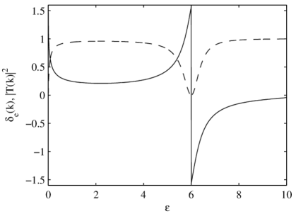
Figure 1: Even scattering phase $\delta_{e}(k)$ (solid line) and transmission probability $|T|^{2}$ (dashed line) of a Feshbach resonance as a function of energy $\varepsilon=k^{2}$ with a resonance at $\varepsilon_{res}=6$. Parameters: $u=10$, $v=-4$ and $g=1$.

3.2 Two-component Feshbach resonances with a contact potential

The quintessential mechanism for a Feshbach resonance occurs, when one couples two internal states $\boldsymbol{\chi}=(\chi_{q},\chi_{p})^{\top}$ to the external motion of the one-dimensional, two-particle Hamiltonian of Eq. (13). The closed q-channel needs an attractive delta potential to support a bound state and a localized coupling matrix element is required to provide an interaction with the open p-channel [34]. A simple, analytically solvable model for this is

$$H=H_{0}(p_{1},p_{2})\otimes\mathds{1}+V(x_{1}-x_{2}),$$

$$V(x)=\left(\begin{array}[]{cc}u+v\delta(x)&g\delta(x)\\ g\delta(x)&0\end{array}\right).$$ (24)

The parameters of the potential matrix $V$ are the threshold energy $u>0$, the strength of the closed channel potential $v<0$ and the channel coupling parameter $g$. As in the scalar case, all contributions to the Hamiltonian are translationally invariant and a product ansatz for the wave-function $\boldsymbol{\chi}_{2}(x_{1},x_{2})=\exp{(iQX)}\boldsymbol{\chi}(x)$ leads to the Schrödinger equation for the relative wave-function

$$\left[\frac{d^{2}}{dx^{2}}+\varepsilon-V(x)\right]{\boldsymbol{\chi}}(x)=0.$$ (25)

Here, we have again introduced rescaled potentials, energies and length mentioned in the context of Eq. (17).

For relative scattering energies $0<\varepsilon(k)=k^{2}<u$, smaller than the threshold energy $u$, the closed channel asymptotic wave-function $\chi_{q}(x)$ vanishes exponentially, while the open channel wave-function $\chi_{p}(x)$ propagates outward freely. Due to the even parity of the contact potential, we can also choose wave-functions of definite parity, i. e.,

$$\lim_{x\rightarrow\pm\infty}\chi_{q}^{(e)}(x,k)\sim e^{-q|x|},\quad q(k)=\sqrt{u-k^{2}},$$ (26)

$$\lim_{x\rightarrow\pm\infty}\chi_{p}^{(e)}(x,k)\sim\cos(kx\pm\delta_{e}).$$ (27)

Odd wavefunctions do not accrue any phase shift, as they vanish at the point of interaction.

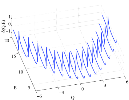
Figure 2: Even scattering phase $\delta_{e}(k(Q,E))$ versus energy $E$ and momentum $Q$. The Feshbach resonances are located on a free space parabola as a function of $Q$. Parameters as in Eq. (36).

By integrating the coupled Schrödinger equation Eq. (25) over an infinitesimal strip around the discontinuity, one obtains the necessary boundary conditions to compute the scattering phase of the even wavefunction. After some minor algebra, one obtains the phase shifts

$$\tan{(\delta_{e})} =-\frac{g^{2}}{2k(2q(k)+v)},\qquad\delta_{o}=0.$$ (28)

This phase shift and the corresponding transmission probability $|T|^{2}$ of Eq. (21) are depicted in Fig. 1. One clearly observes the Feshbach resonance with a $\pi$-phase jump at $\varepsilon_{res}=k^{2}_{res}=u-v^{2}/4$. The position of the resonance energy is usually controlled by changing the dissociation threshold energy $u$ via magnetic fields or via the depth of the bound state $v$, which is an property of the considered atomic element and, thus, harder to modify. The width of the resonance is primarily determined by the coupling strength $g$ [35]. Due to the vanishing odd phase-shift, the total reflection $T=0$ also occurs at the same energy, when the even phase shift reaches $\delta_{e}(k_{res})=\pi/2$. It is also important to note that the phase can be well approximated by a Breit-Wigner curve in the vicinity of the resonance.

In Fig. 2, we present the same scattering phase $\delta_{e}(k(E,Q))$ of Eq. (28), now as a function of the two-particle energy $E$ and the center-of-mass momentum $Q$, according to Eq. (18). This representation emphasizes the parabolic form of the resonance energy $E_{res}=\varepsilon_{res}+Q^{2}/4>0$, as a function of $Q$. The Feshbach resonance is always present for $\varepsilon_{res}>0$ and for all $Q$, or it disappears if $\varepsilon_{res}<0$. As we will show in the following sections, this fundamental behavior can be changed by considering Feshbach scattering in a lattice where center-of-mass and relative motion are coupled. Results can be seen in the final Figs. 11 and 12.

4 Scattering on a one-dimensional lattice

4.1 Bloch states and periodic boundary conditions

Studying physics in periodic structures immediately leads to the consideration of Bloch states [36, 2], which reflect the discrete translation symmetry $\mathcal{D}(la)=\exp{[ilap/\hbar]}$ of the Hamiltonian $[H_{L},\mathcal{D}(la)]=0$ with $l\in\mathds{N}$ . We have already introduced a quasi-one dimensional lattice Hamiltonian in Eq. (7) and will disregard from now on the transverse degrees motion, i. e.,

$$H_{L}(x,p) = \frac{p^{2}}{2m}+U_{L}(x),\quad U_{L}(x)=U_{L}\cos^{2}{(k_{L}x/2)}.$$ (29)

The lattice potential $U_{L}(x+a)=U_{L}(x)$ is characterized by a lattice constant $a$, which in turn defines the crystal momentum $k_{L}=2\pi/a$. Thus, the eigenstates of Schrödinger equations

$$H_{L}|q,n\rangle=\varepsilon_{L}^{n}(q)|q,n\rangle,$$ (30)

can be classified as Bloch states $|{q,n}\rangle$ with quasi momentum $-\pi/a\leq q<\pi/a$, and energy bands $\varepsilon_{L}^{n}(q)$, labeled by band-index $n$. According to the Bloch theorem

$$\langle x\!\mid\!{q,n}\rangle=e^{iqx}u_{q}^{n}(x),\quad u_{q}^{n}(x+a)=u_{q}^{n}(x).$$ (31)

Such an energy eigenfunction can be decomposed into a plane wave phase factor and a lattice periodic function $u_{q}^{n}$. Subjected to translation to the next lattice site, the wave-function acquires a complex phase

$$\langle x+a\!\mid\!{q,n}\rangle=e^{iqa}\langle x\!\mid\!{q,n}\rangle.$$ (32)

The periodic continuation in momentum space has its subtleties and attention needs to be paid to the vanishing of the wave-function at the center or edge of the first Brillouin zone [36]. However, the generic case is simply given by $\langle x\!\mid\!{q+k_{L},n}\rangle=\langle x\!\mid\!{q,n}\rangle$.

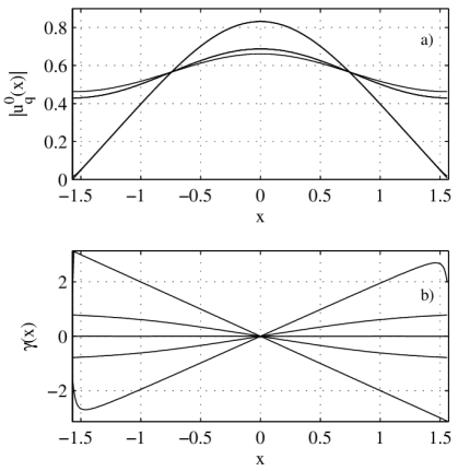
Figure 3: Magnitude $|u_{q}^{0}(x)|$ (a) and phase $\gamma(x)$ (b) of the lowest band Bloch function $\langle x\!\mid\!q,n=0\rangle=|u_{q}^{n}(x)|\exp{[i\gamma(x)]}$, versus dimensionless position $-\pi/2\leq x<\pi/2$, for a few momenta $q=(-1,-0.5,0,0.5,0.992)$. In this shallow potential the Bloch waves are almost plane and deviations are only seen at the band edge $q\approx\pm 1$. Parameters as in Eq. (36).

In practice, it is usually necessary to work with a discrete subset of Bloch states, which are found by considering a periodically continued, finite lattice with an even number of wells $N=2M$. The Born-von-Karman periodic boundary conditions, then require that

$$\langle x+L\!\mid\!{q,n}\rangle=e^{iqL}\langle x\!\mid\!{q,n}\rangle=\langle x\!\mid\!q,n\rangle.$$ (33)

where the total length $L=Na$. This can only be true, if there are exactly $N$ distinct momenta $q_{l}$ in each band

$$-\frac{\pi}{a}\leq q_{l}=\frac{2\pi l}{L}=k_{L}\frac{l}{N}<\frac{\pi}{a},\quad-\frac{N}{2}\leq l<\frac{N}{2}.$$ (34)

We choose the following orthogonalization for the Bloch-states on a finite lattice

$$\langle q_{1},n_{1}\!\mid\!q_{2},n_{2}\rangle=N\delta_{q_{1},q_{2}}\delta_{n_{1},n_{2}},\quad\int_{0}^{a}dx|\langle x\!\mid\!q,n\rangle|^{2}=1.$$ (35)

The general behavior of the Bloch states is shown in Fig. 3. There we have selected a few Bloch eigenfunctions for some momenta $q$ within the Brillouin zone, which exemplify the modified plane wave behavior. A typical energy-band structure in coordinate and momentum space is presented in Fig. 4 and Fig. 5, respectively. In here and all of the following calculations, we use dimensionless parameters for a shallow lattice that only supports one band below the barrier i. e.,

$$U_{L}=-(6/5)^{2},\quad a=\pi,\quad N=2^{8}.$$ (36)

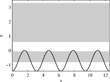
Figure 4: Lattice potential $U_{L}(x)$ (solid line) versus position $x$, superimposed on top of two allowed energy bands $\varepsilon_{L}^{0}(q)$ and $\varepsilon_{L}^{1}(q)$ (shaded gray). Parameters as in Eq. (36).

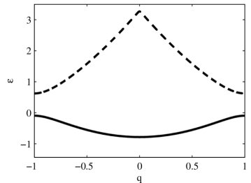
Figure 5: Energy bands $\varepsilon_{L}^{0}(q)$ (solid) and $\varepsilon_{L}^{1}(q)$ (dashed) versus quasi-momentum $q$ in the first Brillouin zone $-1\leq q<1$.

4.2 Scalar two-particle scattering in lattices

We will now consider the scattering of two particles in the presence of a lattice. Thus, we have a two-particle lattice Hamiltonian and a binary interaction $V$

$$H=H_{L}(x_{1},p_{1})+H_{L}(x_{2},p_{2})+V(x_{1}-x_{2}).$$ (37)

By forming two-particle basis states out of single particle Bloch waves one obtains two-dimensional Bloch states

$$|Q,q,n_{1},n_{2}\rangle=|q_{1}(Q,q),n_{1}\rangle\otimes|q_{2}(Q,q),n_{2}\rangle$$ (38)

$$Q=q_{1}+q_{2},\quad q=(q_{1}-q_{2})/2$$ (39)

$$q_{1}=Q/2+q,\quad q_{2}=Q/2-q.$$ (40)

Figure 6: Reciprocal momentum space for two particles in a one-dimensional lattice consisting of only $N=4$ wells. The Cartesian axes represent the individual momenta in the reduced zone scheme $-1\leq q_{1},q_{2}<1$. The $45^{\circ}$ rotated grid lines correspond to the contours of center-of-mass $-1\leq Q<1$ and relative momentum $-1\leq q<1$.

The corresponding reciprocal momentum space for two particles in a one-dimensional lattice is depicted in Fig. 6. One can see the individual single particle momenta $q_{1}$ and $q_{2}$, as well as the center-of-mass momentum $Q$ and relative momentum $q$. This set of symmetry adjusted basis states can be used to represent a general quantum state with quasi-momentum $Q$ as

$$|\chi,Q\rangle=\sum_{q,n_{1},n_{2}}\chi_{Q}^{(n_{1},n_{2})}(q)|Q,q,n_{1},n_{2}\rangle$$ (41)

$$\mathcal{D}_{12}(la)|\chi,Q\rangle=e^{ilaQ}|\chi,Q\rangle.$$ (42)

From the discrete translation symmetry of the system, one finds the selection rule

$$0 =\langle\chi,Q|[H,\mathcal{D}_{12}(la)]|\chi,Q^{\prime}\rangle=\langle\chi,Q|H|\chi,Q^{\prime}\rangle(e^{ila(Q^{\prime}-Q)}-1),$$ (43)

which implies $Q^{\prime}=Q{\rm mod}k_{L}$. In the following, we will consider only transitions within the lowest energy band i. e., $n_{1}=n_{2}=0$ and simplify the notation to $\chi_{Q}^{(0,0)}(q)\equiv\chi_{Q}(q)$, consequently.

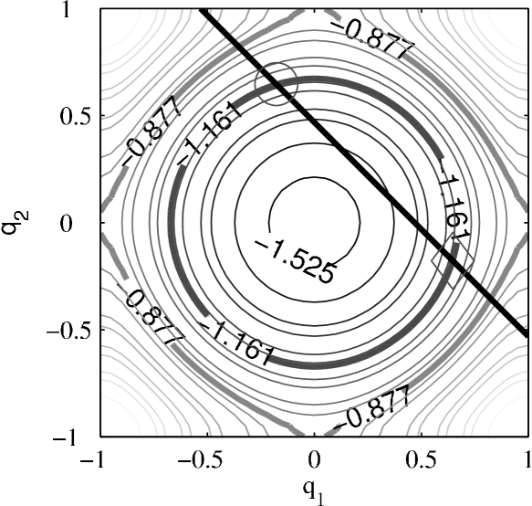
Figure 7: Energy contours $E_{L}(Q,q)$ for the non-interacting two-particle system in momentum space. The superimposed $Q=$const. line (solid black) has two intersections with another $E=$const. contour (dark gray), which are at $q$ (circled) and $-q$ (boxed).

Within these assumptions, one can represent the Schrödinger equation to Eq. (37) as

$$0= \sum_{q^{\prime}}\Big{\{}[\varepsilon_{L}^{0}(q_{1})+\varepsilon_{L}^{0}(q_{2})-E]\delta_{qq^{\prime}}+V_{Q}(q,q^{\prime})\Big{\}}\chi_{Q}(q^{\prime}),$$ (44)

where $q_{1}=q_{1}(Q,q)$ and $q_{2}=q_{2}(Q,q)$. If we let our perturbation tend to zero, then we are left with the two-dimensional energy surface

$$E_{L}(Q,q)=\varepsilon_{L}^{0}(q_{1})+\varepsilon_{L}^{0}(q_{2}).$$ (45)

The contour lines of which are depicted in Fig. 7. The marked intersections show that there are two linearly independent two-particle quantum states labeled by $(q_{1},q_{2})$ and $(q_{2},q_{1})$ that have the same total energy $E$ and center-of-mass momentum $Q$. It it interesting to note that in general there are no straight contour-lines at $Q=\pm 1$ or $q=\pm 1$, as would be the case in the tight binding limit $|U_{L}|\gg 1$. The energy range that is covered by the two-particle energy can be seen in Fig. 8. It shows the projections along the $Q$ and $q$ momentum lines.

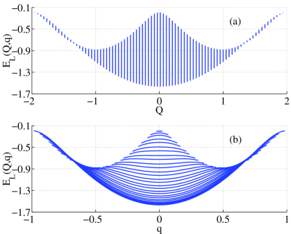
Figure 8: Projections of the two-dimensional energy surface $E_{L}(Q,q)$ versus momentum $Q$ (a) and $q$ (b).

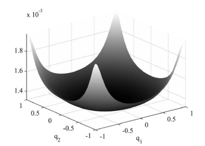
Figure 9: Interaction matrix element $v_{Q}(q,q^{\prime})$ in reciprocal momentum space for $Q=0$, other parameters as in Eq. (36).

Now, if we turn to the evaluation of the matrix element $V_{Q}(q,q^{\prime})$, then it is best expressed in center-of-mass coordinates. Moreover, the algebra simplifies considerable, if we use a zero-range contact potential for the binary potential $V(y)=v\delta(y)$ and obtain

$$V(Q,q,q^{\prime}) = vv_{Q}(q,q^{\prime}),$$ (46)

$$v_{Q}(q,q^{\prime}) = \int_{0}^{a}\frac{dx}{N}\Big{\{}u^{*}_{Q/2+q}(x)u^{*}_{Q/2-q}(x)u_{Q/2+q^{\prime}}(x)u_{Q/2-q^{\prime}}(x)\Big{\}}.$$ (47)

The shape of this potential matrix can be calculated quite accurately with localized Wannier functions in the Gaussian approximations. In general, this agrees well with the numerical results shown in Fig. 9. In this picture, we have chosen a value of $Q=0$ for the center-of-mass momentum. For other values $Q\neq 0$, one obtains a modest variation of the shape of the matrix element at the momentum edges, but it remains predominantly constant inside.

4.3 Two component Feshbach scattering in lattices

Having established the basic notions and concepts in the previous sections, we can now turn to the Feshbach resonance scattering phenomenon in a lattice. The basic Hamiltonians have been already introduced in Eqs. (2), (3.2) and (37). Explicitly, we have the motion in the lattice Hamiltonian $H_{L}$, as well as the Feshbach potential $V$

$$H=H_{L}(x_{1},p_{1},x_{2},p_{2})\otimes\mathds{1}+V(x_{1}-x_{2})$$

$$V(x)=\left(\begin{array}[]{cc}u+v\delta(x)&g\delta(x)\\ g\delta(x)&0\end{array}\right).$$ (50)

Here we have deliberately disregarded the pairing potential $v_{p}=0$, as it only provides a modification to the Feshbach phenomenon. The state of the coupled two-component system in the lowest Bloch band $n=0$ is now defined as

$$|\boldsymbol{\chi},Q\rangle= \sum_{q}\left(\begin{array}[]{cc}\phi_{Q}(q)\\ \psi_{Q}(q)\end{array}\right)|Q,q\rangle,$$ (53)

where we have characterized the state with the momentum $Q$ and labeled the open and closed channels by the molecular $\phi$ and two-fermion wave-function $\psi$ as in Eq. (2).

In order to obtain the Bloch representation of the Schrödinger equation to Eq. (4.3)

$$E|\boldsymbol{\chi},Q\rangle=H|\boldsymbol{\chi},Q\rangle,$$ (54)

we project it on the two-particle Bloch eigenstate and get

$$E\left(\begin{array}[]{cc}\phi_{Q}(q)\\ \psi_{Q}(q)\end{array}\right)=\sum_{q^{\prime}}\Big{\{}[\varepsilon_{L}^{0}(q_{1}(Q,q))+\varepsilon_{L}^{0}(q_{2}(Q,q))]\delta_{q,q^{\prime}}$$ (57)

$$\left.+\delta_{qq^{\prime}}\left(\begin{array}[]{cc}u&0\\ 0&0\end{array}\right)+v_{Q}(q,q^{\prime})\left(\begin{array}[]{cc}v&g\\ g&0\end{array}\right)\right\}\left(\begin{array}[]{c}\phi_{Q}(q^{\prime})\\ \psi_{Q}(q^{\prime})\end{array}\right).$$ (64)

We have numerically diagonalized this Schrödinger equation for the lattice parameters of Eq. (36) and the Feshbach parameters $u=1.5$, $v=-7$, $g=0.03$. Due to the parity of the Hamiltonian, one can sort the resulting $2N$ eigenstates into even and odd states and assign them a positive or negative quantum index $-N\leq\nu<N$. By turning off the coupling between the manifolds i. e., $g=0$, one can distinguish easily the eigenvalues $E_{\nu}(Q,g=0)$ that belong to molecular (q-channel) or the open fermionic spectrum (p-channel). We have depicted a few representative values in Fig. 10a). It can be seen clearly that there is a single bound state embedded in the allowed energy band of the open p-channel. In Fig. 10b), we present the interacting eigenvalues $E_{\nu}(Q,g=0.03)$, which are now formed by admixtures of both manifolds and can only be distinguished by the parity of the state.

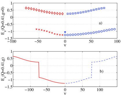
Figure 10: Discrete eigenenergies $E_{\nu}(Q,g)$ versus quantum number $-N\leq\nu<N$ for momentum $Q=0.41$. Negative quantum numbers label odd states, while positive numbers count even states. a) Energies of uncoupled system $E_{\nu}(Q,g=0)$. Note the location of the bound state ($\ast$) of the molecular manifold ($\Diamond$, $\square$) is inside the fermionic spectrum marked by ($\times$, $\circ$). b) All interacting eigenenergies $E_{\nu}(Q,g=0.03)$ versus quantum index $\nu$. Odd states (solid) and even states (dashed dotted). The bound state is now an admixture of molecular and fermionic manifolds.

In order to describe the scattering resonance, we use the standing wave version of the Lippman-Schwinger equation [5]

$$|\boldsymbol{\chi}^{(s)},Q,q\rangle=\mathbf{e}_{p}\otimes|Q,q\rangle+G^{(s)}_{L}(E)V|\boldsymbol{\chi}^{(s)},Q,q\rangle,$$ (65)

where $\mathbf{e}_{p}\otimes|Q,q\rangle$ represents a non-interacting Bloch-wave in the asymptotically open p-channel $\mathbf{e}_{p}=(0,1)^{\top}$. For the lattice Hamiltonian $H_{L}$, one obtains a standing wave Greens function $G^{(s)}_{L}$ from the usual retarded and advanced Greens functions $G^{(\pm)}_{L}$ by

$$G^{(s)}_{L}(E) =\frac{1}{2}(G^{(+)}_{L}(E)+G^{(-)}_{L}(E)),$$ (66)

$$G^{(\pm)}_{L}(E) =\lim_{\epsilon\rightarrow 0+}\frac{1}{E\pm i\epsilon-H_{L}}.$$ (67)

Finally, the effect of scattering is measured by the off-shell Heitler- or K-matrix element

$$K_{Q}(q^{\prime},q)=\langle Q,q^{\prime}|\mathbf{e}_{p}^{\top}V|\boldsymbol{\chi}^{(s)},Q,q\rangle.$$ (68)

We assign an even on-energy shell scattering phase shift

$$\tan{[\delta_{e}(Q,E)]}=K_{Q}(q,q^{\prime}),\quad E=E(Q,q)=E(Q,q^{\prime}).$$ (69)

We have evaluated this phase shift for two differently strong bound molecular states and varied the center-of-mass momentum of the two-particle collision. In the first Fig. 11, one can see the Feshbach resonance cutting into the energy band and disappearing once it is outside. This is modified in Fig. 12, which has a lesser bound resonance, and therfore does not leave at the lower band edge.

This has to be compared with the Feshbach scattering in homogeneous space according to Eq. (28) and has been presented already in Fig. 2. There, the resonance energy $E=\varepsilon_{res}+Q^{2}/4>0$, is on a simple parabola as a function of $Q$. If we tune the Feshbach resonance energy $\varepsilon_{res}<0$, it either disappears completely or is always present.

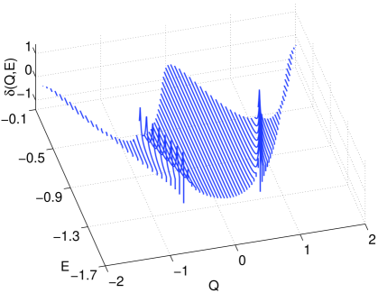
Figure 11: Even scattering phase-shift $\delta_{e}(E,Q)$ of a two-particle Bloch-wave versus energy $E$ and momentum $Q$. Once can see clearly Feshbach resonances symmetrically located around the $Q$-axis, which disappears when the bound state is outside the band. Parameters: $u=1.5$, $v=-7$, $g=0.03$.

5 Experimental considerations

Starting from a dilute Fermi gas, atoms can be loaded adiabatically into the lowest energy band of the lattice. For quasi-momenta not too close to the band edge, this requires that the Fermi energy remains clearly below the atomic recoil energy $\hbar\omega_{r}$, corresponding to 2$\pi\cdot 8.4$ kHz and 2$\pi\cdot 74$ kHz for the ⁴⁰K and ⁶Li D2-lines respectively . To ensure that the Feshbach resonance provides coupling only within a single energy band, its width has to be sufficiently narrow, i. e., below a value of about $\hbar\omega_{r}/\Delta\mu,$ where $\Delta\mu$ denotes the difference of the atomic and the molecular states magnetic moments respectively. For typical parameters, we arrive at a required width of the Feshbach resonance below 10 to 100 mG. We are aware, that the investigation of such weak Feshbach resonances requires a high magnetic field stability. On the other hand, three-body losses, which for free space experiments are a mayor second experimental constraint in the study of narrow Feshbach resonances, are expected to be reduced in the presence of the lattice potential due to atom localization in the micropotentials.

For an experimental verification of the relative atomic momentum dependence of the Feshbach resonance, as indicated in Figs. 11 and 12, one could study such scattering resonances for a variable filling of the lowest energy band in the lattice. In this way, due to the Pauli exclusion principle, for an increased band filling different regions of the relative atomic quasi-momentum are subsequently filled up. The variation of the lineshape of the Feshbach resonance is determined by the collisional properties of atoms in the lattice. For example, if we take the situation of Fig. 11, for small atom filling the scattering resonance would disappear. The Feshbach resonance here could only be observed for a large atom filling.

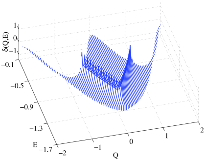
Figure 12: Even scattering phase-shift $\delta_{e}(E,Q)$ of a two-particle Bloch-wave versus energy $E$ and momentum $Q$. With a less deeply bound state the resonances remain above the lower band edge. Parameter: $u=1.5$, $v=-5$, $g=0.03$.

6 Conclusions and Outlook

We have considered Feshbach scattering of two Fermions in a one-dimensional optical lattice. Due to the reduction of translation invariance, the relative and center-of-mass motion are coupled and we present the scattering theory in the crystal momentum basis. Within a single band approximation, we have calculated numerically Feshbach resonances and demonstrate that the position of the Feshbach resonance depends selectively on the center-of-mass momentum, due to the non-parabolic shape of the energy band. The simple resonance structure suggests that a semi-analytical calculation based on an effective-mass approximation should be applicable and is currently pursued.

In the present article, we have only considered Feshbach resonances that are much weaker than the interband separation. Thus, we could limit the discussion to a single energy band. Wider Feshbach resonances will involve the coupling of several bands. Going beyond the single band approximations will provide interesting new physics as already advanced in Ref. [25] for the case of potential scattering. This will be examined, based on the present formulation, in a forthcoming publication.

References

References

- [1] J. Slater. Interaction of waves in crystals. Rev. Mod. Phys., 30:197, 1958.
- [2] J. Callaway. Quantum theory of the solid state. Academic Press, 1991.
- [3] B. Batterman and H. Cole. Dynamical diffraction of x rays by perfect crystals. Rev. Mod. Phys., 36:681, 1964.
- [4] C. Cohen-Tannoudji. Atomic motion in laser light. In J. Dalibard, J. Raimond, and J. Zinn-Justin, editors, Le Houches Lecture Notes, Course XXX, Fundamental Systems in Quantum Optics. Elsevier Science Publishers, 1990.
- [5] J. Taylor. Scattering Theory. Dover Publications, 2000.
- [6] M. Weitz, G. Cennini, G. Ritt, and C. Geckeler. Optical multiphoton lattices. Phys. Rev. A, 70:043414, 2004.
- [7] D. Jaksch, C. Bruder, J. Cirac, C. Gardiner, and P. Zoller. Cold bosonic atoms in optical lattices. Phys. Rev. Lett., 81:3108, 1998.
- [8] C. Kollath, U. Schollwöck, J. von Delft, and W. Zwerger. Spatial correlations of trapped one-dimensional bosons in an optical lattice. Phys. Rev. A, 69:31601, 2004.
- [9] I. Bloch. Ultracold quantum gases in optical lattices. Nature Physics, 1:23, 2005.
- [10] O. Morsch and M. Oberthaler. Dynamics of bose-einstein condensates in optical lattices. Rev. Mod. Phys., 78:179, 2006.
- [11] M. Rigol, A. Muramatsu, G. Batrouni, and R. Scalettar. Local quantum criticality in confined fermions on optical lattices. Phys. Rev. Lett., 91:130403, 2003.
- [12] M. Rigol and A. Muramatsu. Quantum monte carlo study of confined fermions in one-dimensional optical lattices. Phys. Rev. A, 69:053612, 2004.
- [13] M. Köhl, H. Moritz, Th. Stöferle, K. Günter, and T. Esslinger. Fermionic atoms in a three dimensional optical lattice: Observing fermi surfaces, dynamics, and interactions. Phys. Rev. Lett., 94:080403, 2005.
- [14] G. Orso and G. Shlyapnikov. Superfluid fermi gas in a 1d optical lattice. Phys. Rev. Lett., 95:260402, 2005.
- [15] L. Carr and M. Holland. Quantum phase transitions in the fermi-bose hubbard model. Phys. Rev. A, 72:031604, 2005.
- [16] C. Ospelkaus, S. Ospelkaus, L. Humbert, P. Ernst, K. Sengstock, and K. Bongs. Ultracold heteronuclear molecules in a 3d optical lattice. Phys. Rev. Lett., 97:120402, 2006.
- [17] D. B. Dickerscheid and H. T. Stoof. Feshbach molecules in a one-dimensional fermi gas. Phys. Rev. A, 72:053625, 2005.
- [18] G. Orso, L. P. Pitaevskii, S. Stringari, and M. Wouters. Formation of molecules near a feshbach resonance in a 1d optical lattice. Phys. Rev. Lett., 95:060402, 2005.
- [19] Th. Stöferle, K. Günter H. Moritz, M. Köhl, and T. Esslinger. Molecules of fermionic atoms in an optical lattice. Phys. Rev. Lett., 96:030401, 2006.
- [20] K. Winkler, G. Thalhammer, F. Lang, R. Grimm, J. Hecker Denschlag, A. J. Daley, A. Kantian, H. P. Büchler, and P. Zoller. Repulsively bound atom pairs in an optical lattice. Nature, 441:853, 2006.
- [21] M. Wouters and G. Orso. Two-body problem in periodic potentials. Phys. Rev. A, 73:012707, 2006.
- [22] M. Grupp, G. Nandi, R. Walser, and W.P. Schleich. Collective feshbach scattering of a superfluid droplet from a mesoscopic two-component bose-einstein condensate. Phys. Rev. A, 73:50701, 2006.
- [23] E. Adams. Motion of an electron in a perturbed electronic potential. Phys. Rev., 85:41, 1952.
- [24] E. Tiesinga, A. Moerdijk, B. Verhaar, and H. Stoof. Conditions for bose-einstein condensation in magnetically trapped atomic cesium. Phys. Rev. A, 46:1167, 1992.
- [25] R. Diener and T. Ho. Fermions in optical lattices swept across feshbach resonances. Phys. Rev. Lett., 96:010402, 2006.
- [26] C. Regal, C. Ticknor, J. Bohn, and D. Jin. Creation of ultracold molecules from a fermi gas of atoms. Nature, 424:47, 2003.
- [27] C. Chin, M. Bartenstein, A. Altmeyer, S. Riedl, S. Jochim, J. Hecker Denschlag, and R. Grimm. Observation of the pairing gap in a strongly interacting fermi gas. Science, 305:1128, 2004.
- [28] M. Zwierlein, C. Stan, C. Schunck, S. Raupach, A. Kerman, and W. Ketterle. Condensation of pairs of fermionic atoms near a feshbach resonance. Phys. Rev. Lett., 92:120403, 2004.
- [29] M. Holland, S.J.J.M.F. Kokkelmans, M. Chiofalo, and R. Walser. Resonance superfluidity in a quantum degenerate fermi gas. Phys. Rev. Lett., 87:120406, 2001.
- [30] S. Kokkelmans, J. Milstein, ML. Chiofalo, R. Walser, and M. Holland. Resonance superfluidity: Renormalization of resonance scattering theory. Phys. Rev. A, 65:053617, 2002.
- [31] U. Fano. Effects of configuration interaction on intensities and phase shifts. Phys. Rev., 124:1866, 1961.
- [32] H. Feshbach. A unified theory of nuclear reactions. Ann. Phys., 5:357, 1958.
- [33] H. Feshbach. A unified theory of nuclear reactions. II. Ann. Phys., 19:287, 1962.
- [34] D. Bilhorn and W. Tobocman. Coupled square well model for elastic scattering. Phys. Rev., 122:1517, 1961.
- [35] H. Friedrich. Theoretische Atomphysik. Springer Verlag, Berlin, 1990.
- [36] W. Kohn. Analytic properties of bloch waves and wannier functions. Phys. Rev., 115:809, 1959.