MHD simulations of the magnetorotational instability in a shearing box with zero net flux. II. The effect of transport coefficients

Abstract

Aims. We study the influence of the choice of transport coefficients (viscosity and resistivity) on MHD turbulence driven by the magnetorotational instability (MRI) in accretion disks.

Methods. We follow the methodology described in paper I: we adopt an unstratified shearing box model and focus on the case where the net vertical magnetic flux threading the box vanishes. For the most part we use the operator split code ZEUS, including explicit transport coefficients in the calculations. However, we also compare our results with those obtained using other algorithms (NIRVANA, the PENCIL code and a spectral code) to demonstrate both the convergence of our results and their independence of the numerical scheme.

Results. We find that small scale dissipation affects the saturated state of MHD turbulence. In agreement with recent similar numerical simulations done in the presence of a net vertical magnetic flux, we find that turbulent activity (measured by the rate of angular momentum transport) is an increasing function of the magnetic Prandtl number $Pm$ for all values of the Reynolds number $Re$ that we investigated. We also found that turbulence disappears when the Prandtl number falls below a critical value $Pm_{c}$ that is apparently a decreasing function of $Re$. For the limited region of parameter space that can be probed with current computational resources, we always obtained $Pm_{c}>1$.

Conclusions. We conclude that the magnitudes of the transport coefficients are important in determining the properties of MHD turbulence in numerical simulations in the shearing box with zero net flux, at least for Reynolds numbers and magnetic Prandtl numbers that are such that transport is not dominated by numerical effects and thus can be probed using current computational resources.

1 Introduction

To date, the magnetorotational instability (MRI) is believed to be the most likely cause of anomalous angular momentum transport in accretion disks (Balbus & Hawley 1998). The results of numerous numerical simulations carried out over the last 15 years indicate that the MRI results in MHD turbulence that transports angular momentum outwards with rates that seem, depending on the net magnetic flux present, to be compatible to order of magnitude with those estimated from the observations. Most of these studies were local MHD numerical simulations of a shearing box performed using finite difference methods. Unfortunately because of the limited computational resources available during the 90’s, these early calculations were restricted to low and moderate resolutions, having at most $64$ grid cells per disk scale height (Hawley et al. 1995, 1996; Fleming et al. 2000; Sano et al. 2004).

In paper I (Fromang & Papaloizou 2007), we used one of these numerical codes, ZEUS (Hawley & Stone 1995), to study the convergence of the results as the grid resolution is increased. We explored resolutions ranging from $64$ to $256$ grid cells per scale height and concentrated on the special case for which the net vertical flux threading the box vanishes. We found that the angular momentum transport, measured using the standard $\alpha$ parameter, decreases linearly with the grid spacing as the resolution increases. In the best resolved simulations, we obtained $\alpha=10^{-3}$, which amounts to a decrease of about one order of magnitude when compared to the earlier estimates derived from the first simulations of this problem (Hawley et al. 1995). This situation comes about because significant flow energy and dissipation occurring at the grid scale affects the numerical results, at least for the resolutions that can currently be achieved.

Since the diffusive transport and dissipation that plays an important role in determining the outcome is purely numerical in ZEUS, we concluded that explicit physical dissipation, both viscous and resistive, should be properly included in the simulations for them to show numerical convergence and thus have physical significance. The purpose of this paper is to investigate the effect of specified transport coefficients on the saturated state of MRI driven MHD turbulence.

We note that this issue has recently been considered by Lesur & Longaretti (2007) for cases for which a nonzero net vertical flux threads the disk. They found that both the viscosity $\nu$ and the resistivity $\eta$ affect the amount of angular momentum transported by MHD turbulence, in such a way that $\alpha$ increases with the magnetic Prandtl number $Pm=\nu/\eta$. One of the aims of this paper is to investigate whether such a relation exists in the absence of net flux and to quantify the precise rate of angular momentum transport for that case as a function of the transport coefficients.

The plan of the paper is as follows. In section 2, we describe our numerical setup and the models we simulated. Section 3 focuses on the properties of one of these models. Specifically, we demonstrate that for the simulations performed with ZEUS, numerical dissipation does not strongly affect the results when explicit transport coefficients of sufficient magnitude are included. This is done by using Fourier analysis as introduced in paper I, and by comparing the simulation results obtained using a variety of numerical schemes. Having validated our approach, we turn in section 4 to a more systematic exploration of the parameter space. We recover the correlation between $\alpha$ and $Pm$ mentioned above and surprisingly identify a regime of parameters in which MHD turbulence decays. Finally, we discuss our results, their limits and their astrophysical implications in section 5.

2 Model properties

As in paper I, we work in the framework of the shearing box model (Goldreich & Lynden-Bell 1965). The standard ideal MHD equations are modified to account for small scale dissipation resulting from finite and constant viscosity $\nu$ and resistivity $\eta$. For clarity they are recalled below.

$$\frac{\partial\rho}{\partial t}+\mbox{\boldmath{$\nabla$}}\mbox{\boldmath{$\cdot$}}(\rho\mbox{\boldmath{$v$}}) = 0\,,$$ (1)

$$\rho\frac{\partial\mbox{\boldmath{$v$}}}{\partial t}+\rho(\mbox{\boldmath{$v$}}\mbox{\boldmath{$\cdot$}}\mbox{\boldmath{$\nabla$}})\mbox{\boldmath{$v$}}+2\rho\mbox{\boldmath{$\Omega$}}\times\mbox{\boldmath{$v$}} = \frac{(\mbox{\boldmath{$\nabla$}}\mbox{\boldmath{$\times$}}\mbox{\boldmath{$B$}})\mbox{\boldmath{$\times$}}\mbox{\boldmath{$B$}}}{4\pi}-\mbox{\boldmath{$\nabla$}}P+\nabla\mbox{\boldmath{$\cdot$}}\mbox{\boldmath{$T$}},$$ (2)

$$\frac{\partial\mbox{\boldmath{$B$}}}{\partial t} = \mbox{\boldmath{$\nabla$}}\mbox{\boldmath{$\times$}}(\mbox{\boldmath{$v$}}\mbox{\boldmath{$\times$}}\mbox{\boldmath{$B$}}-\eta\mbox{\boldmath{$\nabla$}}\mbox{\boldmath{$\times$}}\mbox{\boldmath{$B$}})\,.$$ (3)

As in paper I, $\Omega$ is the Keplerian angular velocity at the centre of the box, $\rho$ is the gas density, $v$ is the velocity, $B$ is the magnetic field and $P$ is the pressure. This is related to the gas density and the constant speed of sound $c_{0}$ through the isothermal equation of state $P=\rho c_{0}^{2}.$ We adopt a Cartesian coordinate system $(x,y,z)\equiv(x_{1},x_{2},x_{3})$ with associated unit vectors $(\mbox{\boldmath{$i$}},\mbox{\boldmath{$j$}},\mbox{\boldmath{$k$}}).$

Viscosity enters the equations through the viscous stress tensor $T$ whose components are defined following Landau & Lifshitz (1959)

$$T_{ik}=\rho\nu\left(\frac{\partial v_{i}}{\partial x_{k}}+\frac{\partial v_{k}}{\partial x_{i}}-\frac{2}{3}\delta_{ik}\mbox{\boldmath{$\nabla$}}\mbox{\boldmath{$\cdot$}}\mbox{\boldmath{$v$}}\right)\,.$$ (4)

As in paper I, the simulations are performed within a box with dimensions $(L_{x},L_{y},L_{z})=(H,\pi H,H)$, where $H=c_{0}/\Omega$ is the disk scale height. Throughout this paper, we used the resolutions $(N_{x},N_{y},N_{z})=(128,200,128)$ or $(256,400,256)$ depending on the magnitude of the dissipation coefficients. All the simulations are initialised with the same density and magnetic field as in paper I. The initial velocity is taken to be given by the Keplerian shear with the addition of a random perturbation of small amplitude to each component. As in paper I, we measure time in units of the orbital period $2\pi/\Omega$.

Model	Resolution	Reynolds number	Pm	$\alpha_{Rey}$	$\alpha_{Max}$	$\alpha$	Turbulence?
128Re800Pm4	$(128,200,128)$	800	4	-	-	-	No
128Re800Pm8	$(128,200,128)$	800	8	$5.8\times 10^{-3}$	$2.6\times 10^{-2}$	$3.1\times 10^{-2}$	Yes
128Re800Prm16	$(128,200,128)$	800	16	$8.1\times 10^{-3}$	$3.6\times 10^{-2}$	$4.4\times 10^{-2}$	Yes
128Re1600Pm2	$(128,200,128)$	1600	2	-	-	-	No
128Re1600Pm4	$(128,200,128)$	1600	4	$1.6\times 10^{-3}$	$8.1\times 10^{-3}$	$9.7\times 10^{-3}$	Yes
128Re1600Pm8	$(128,200,128)$	1600	8	$3.3\times 10^{-3}$	$1.6\times 10^{-2}$	$1.9\times 10^{-2}$	Yes
128Re3125Pm1	$(128,200,128)$	3125	1	-	-	-	No
128Re3125Pm2	$(128,200,128)$	3125	2	-	-	-	No
128Re3125Pm4	$(128,200,128)$	3125	4	$1.6\times 10^{-3}$	$7.4\times 10^{-3}$	$9.1\times 10^{-3}$	Yes
128Re6250Pm1	$(128,200,128)$	6250	1	-	-	-	No
128Re6250Pm2	$(128,200,128)$	6250	2	-	-	-	No
128Re12500Pm1	$(128,200,128)$	12500	1	-	-	-	No
256Re12500Pm2	$(256,400,256)$	12500	2	$3.2\times 10^{-4}$	$1.3\times 10^{-3}$	$1.6\times 10^{-3}$	Yes
256Re25000Pm1	$(256,400,256)$	25000	1	-	-	-	No

Table 1: Properties of the simulations presented in this paper and performed with the finite difference code ZEUS. The first column gives the label of the model while the resolution $(N_{x},N_{y},N_{z})$ is specified in the second column. The third column gives the Reynolds number associated with the viscosity , $(c_{0}H)/\nu),$ and the fourth column gives the magnetic Prandtl number $Pm$. The following three columns quantify the amount of turbulent activity, when nonzero, through the values of $\alpha_{Rey}$, $\alpha_{Max}$ and $\alpha$. Finally, the last column describes the outcome, turbulent or not, of each model.

The parameters for the simulations we performed with ZEUS are given in Table 1. In section 3.2, we explore the sensitivity of some of these results to the numerical algorithm by performing a few additional runs using other codes. The details of these simulations as well as the properties of those codes are described there. In Table 1, we give the label of each model in the first column and the resolution $(N_{x},N_{y},N_{z})$ in the second column. As mentioned above, the models include explicit viscosity and resistivity, the values of these can be found from the Reynolds number $Re$ (given in the third column) and the magnetic Prandtl number $Pm$ (given in the fourth column). The former is defined by

$$Re=\frac{c_{0}H}{\nu}\,$$ (5)

while the latter, already mentioned in the introduction, quantifies the relative importance of ohmic and viscous diffusion:

$$Pm=\frac{\nu}{\eta}=\frac{Re_{M}}{Re}\,$$ (6)

where the magnetic Reynolds number $Re_{M}=c_{0}H/\eta.$

The aim of this paper is to study the properties of MHD turbulence in each of these models. Table 1 summarise the results by giving, for each of them, the rate of angular momentum transport that MHD turbulence, when present, generates. This is done through specifying the Reynolds stress parameter, $\alpha_{Rey},$ the Maxwell stress parameter $\alpha_{Max}$ and the total stress parameter $\alpha$ in columns five, six and seven respectively. These represent actual stresses normalised by the initial thermal pressure. They are defined precisely in paper I through Eq. (6), (7) and (8). As will be emphasised below, some models fail to show sustained turbulence. This is why the last column of Table 1 describes the nature, turbulent or not, of the flow for each model. For cases in which MHD turbulence is found to decay, no stress parameters are given.

3 Re=3125, Pm=4

3.1 Simulation set up

In this section, we concentrate on the particular model 128Re3125Pm4 for which $Re=3125$ and $Pm=4$ in order to describe common features characterising simulations of this type. Model 128Re3125Pm4 was computed for a duration of 440 orbits using ZEUS with a resolution $(N_{x},N_{y},N_{z})=(128,200,128)$. When using this code, it is important to be sure that dissipation arising from the specified diffusion coefficients $\nu$ and $\eta$ dominates that due to numerical effects. This is verified in section 3.1.2 using the Fourier analysis described in paper I. We also compare the results from model 128Re3125Pm4 to results obtained from similar models computed using other numerical methods (see section 3.2). This shows that the results obtained in the present paper are independent of the numerical scheme used. But before considering these points in detail, we first describe the overall properties of model 128Re3125Pm4.

3.1.1 Simulation properties

Figure 1: Time history of $\alpha_{Re}$ (dotted line), $\alpha_{Max}$ (dashed line) and $\alpha$ (solid line) for model 128Re3125Pr4. From the rate of angular momentum transport averaged between $t=40$ and the end of the simulation we obtain $\alpha=9.1\times 10^{-3}$.

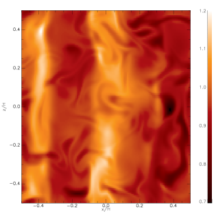
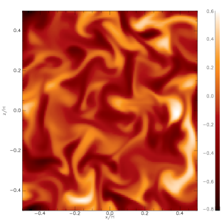
Figure 2: Snapshot of the density (left panel) and of the y component of the magnetic field (right panel) in the $(x,z)$ plane for model 128Re3125Pm4. In the former case, the local density is normalised by the mean density in the box. In the latter case, the magnetic field is normalised by the square root of the mean thermal pressure in the box.

Despite effects arising from the specification of nonzero dissipation coefficients, the overall evolution of model 128Re3125Pm4 is qualitatively very similar to that found in numerical simulations of MHD turbulence in the shearing box since the early $1990$’s. The MRI destabilises the flow, which causes the Maxwell and Reynolds stresses to grow exponentially during the first few orbits. When the disturbance reaches a large enough amplitude, the instability enters the non linear regime, the flow breaks down into MHD turbulence and eventually settles into a quasi steady state during which angular momentum is transported outwards. The rate of angular momentum transport is illustrated in figure 1 which shows the time history of $\alpha_{Rey}$ (dotted line), $\alpha_{Max}$ (dashed line) and $\alpha$ (solid line). Averaging $\alpha$ in time between $t=40$ and the end of the simulation, we find $\alpha=9.1\times 10^{-3}$. As with simulations done without including explicit dissipation coefficients, the transport is dominated by the Maxwell stress, which is found to be roughly $5$ times larger than the Reynolds stress. As in paper I, we checked that the shearing box boundary conditions did not introduce any spurious net flux in the y and z directions. To do so, we measured the maximum value reached by the mean magnetic field components in the box and translated their resulting strengths into effective $\beta$. This gave $\beta_{y}=5.0\times 10^{6}$ and $\beta_{z}=5.6\times 10^{6}$ respectively for the azimuthal and vertical mean components. These values are comparable to the same quantities obtained in paper I in the absence of dissipation coefficients and correspond to field strength far too small to play a role in the model evolution.

In order to illustrate the properties of the flow in this model, in figure 2 we show two snapshots which represent the density (left panel) and azimuthal component of the magnetic field, $B_{y},$ (right panel) in the $(x,z)$ plane at time $t=115.$ As usual with such simulations (whether or not explicit dissipation coefficients are included), density waves develop and propagate radially in the disk. They are superposed on smaller scale fluctuations correlated with the magnetic field fluctuations seen on the right side of Fig. 2. Note, however, the larger characteristic scale of these fluctuations compared to those found in a simulation having the same resolution and no explicit dissipation coefficients (a typical snapshot from such a simulation is available in the middle panel of Fig.4 in paper I). This is because resistivity and viscosity sets a typical dissipation length scale that is larger than a grid cell. This is a first indication that explicit dissipation dominates over numerical dissipation in this simulation. A more quantitative demonstration can be obtained from the Fourier analysis approach of paper I. This is considered in the next section.

3.1.2 Fourier analysis

Figure 3: Variation of $S$ (upper solid line), $T_{bb}$ (dashed line), $T_{divv}$ (dotted line), $T_{bv}$ (dotted–dashed line) and $D_{phys}$ (lower solid line) as functions of the modulus of the wavenumber $k$ for model 128Re3125Pm4. Only $S$ is always positive. As explained in the text, this accounts for the rate of toroidal magnetic field generation by the mean shear flow acting on the poloidal field.

Figure 4: As in figure 3 but for the analogue of Eq. (7) derived from the poloidal components of the induction equation. This shows that poloidal magnetic field energy is created at all scales through field line stretching due to the turbulent velocity fluctuations.

Figure 5: The numerical dissipation rate is plotted vs $k$ using the solid line. This can be compared with the physical dissipation rate per unit volume indicated using the dashed line. The latter has a larger amplitude than the former, indicating that the results are not strongly affected by numerical dissipation.

In paper I, we found that the dynamical properties of the turbulence could be studied in Fourier space. The induction equation leads to a balance between $5$ terms, describing forcing by the mean and turbulent flow, transport to smaller scales, compressibility and numerical dissipation. This gives rise to Eq. (22) of paper I. A similar balance involving $6$ terms can be obtained when explicit resistivity is included. Using the same notation as in paper I, we find

$$S+T_{bb}+T_{divv}+T_{bv}+D_{phys}+D_{num}=0\,.$$ (7)

Here $D_{phys}$ describes physical dissipation per unit volume in ${\bf k}$ space and is defined by

$$D_{phys}=\eta k^{2}|\mbox{\boldmath{$B$}}(k)|^{2}\,,$$ (8)

in which $k$ stands for the modulus of the wavenumber ${\bf k}\equiv(k_{x},k_{y},k_{z}).$ As in paper I, $S$ describes how the background shear creates the y component of the magnetic field, $T_{bb}$ is a term that accounts for magnetic energy transfer toward smaller scales, $T_{divv}$ is due to compressibility, $T_{bv}$ describes how magnetic field is created due to field line stretching by the turbulent flow and $D_{num}$ describes numerical dissipation.

The variation of the first five terms of Eq. (7) with $k$ is plotted in figure 3 (to compute these curves, the simulation data were averaged in time using $100$ snapshots spanning $400$ orbits). $S$ is shown using the upper solid line, the dashed line corresponds to $T_{bb}$ while $T_{divv}$, $T_{bv}$ and $D_{phys}$ are respectively represented using the dotted line, dotted–dashed line and lower solid line respectively. As in paper I, the above quantities are Fourier transforms evaluated with $k_{y}=0$ that are then averaged over the circle $k_{x}^{2}+k_{z}^{2}={\rm constant.}$

In agreement with the results presented in paper I for simulations performed without explicit dissipation, figure 3 shows that the only always positive term is $S$, which is simply due to the fact that toroidal magnetic energy is created by the mean background shear. As in paper I, we next turn to the poloidal part of Eq. (7). This is done by considering only the components of the induction equation for the poloidal part $\mbox{\boldmath{$B$}}_{p}=(B_{x},0,B_{z})$ of the magnetic field $B$. In that case $S$ vanishes. The variation with $k$ of the four remaining terms ($T_{bb}$, $T_{bv}$, $T_{div}$ and $D_{phys}$) is shown on figure 4 using the same conventions as in Fig. 3. Again, the results we obtained are qualitatively similar to the results of paper I. Poloidal magnetic energy is created on a large range of scales by field line stretching, as indicated by the fact that $T_{bv}$ is positive. The other terms are negative and describe transport to smaller scales and dissipation. For the simulation to be converged, physical dissipation need to be larger than numerical dissipation. The interest of this Fourier analysis is to provide a means to test this condition. Indeed, numerical dissipation can be computed as minus the sum of the four terms plotted on figure 4. Its variation with $k$ is shown in figure 5 with the solid line and compared to $D_{phys},$ represented using a dashed line. At small scales ($k$ larger than $30$), numerical dissipation is clearly smaller than physical dissipation. For the smallest $k$, large amplitude fluctuations around zero are observed. They are due to poorer statistics that prevent the procedure from converging everywhere. Nevertheless, figure 5 provides confidence that the dissipation is largely physical in model 128Re3125Pm4. This is also consistent with the results of paper I, which estimated a numerical magnetic Reynolds number of the order of $30000$ at that resolution, significantly larger than the value $Re_{M}=12500$ used in the present model (although we add a note of caution that this estimated value depends on the flow itself and could thus be slightly different here).

3.2 Code comparison

Code	Resolution	Box size	$\alpha_{Rey}$	$\alpha_{Max}$	$\alpha$
ZEUS	$(128,200,128)$	$(H,\pi H,H)$	$1.6\times 10^{-3}$	$7.4\times 10^{-3}$	$9.1\times 10^{-3}$
NIRVANA	$(128,200,128)$	$(H,\pi H,H)$	$1.7\times 10^{-3}$	$7.8\times 10^{-3}$	$9.5\times 10^{-3}$
SPECTRAL CODE	$(64,128,64)$	$(H,\pi H,H)$	$1.4\times 10^{-3}$	$9.4\times 10^{-3}$	$1.1\times 10^{-2}$
PENCIL CODE	$(128,200,128)$	$(H,\pi H,H)$	$1.4\times 10^{-3}$	$6.8\times 10^{-3}$	$8.2\times 10^{-3}$

Table 2: Details of the runs performed using different codes as a way of checking the results for model 128Re3125Pm4. The first three columns respectively describe the code used, the resolution $(N_{x},N_{y},N_{z})$ and the box size $(L_{x},L_{y},L_{z})$. The last three columns summarise the outcome by giving the time averaged values of $\alpha_{Rey}$, $\alpha_{Max}$ and $\alpha$ (averaged between $t=40$ and the end of each simulation). Note that the first line simply recalls the results of model 128Re3125Pm4 which can also be found in Table 1. All models have $Re=3125$ and $Pm=4$.

Figure 6: Results obtained with NIRVANA (left panel), a spectral code (middle panel) and the PENCIL code (right panel) for the comparison case. All panels display the time history of $\alpha_{Rey}$, $\alpha_{Max}$ and $\alpha$ using the same conventions as figure 1, with which they should be compared. Good agreement is found for model 128Re3125Pm4 regardless of the numerical scheme used.

In order to gain further confidence that the results for model 128Re3125Pm4 are not strongly affected by numerical dissipation or numerical details such as, for example, the boundary conditions, we reproduced that simulation using three other codes: NIRVANA (Ziegler & Yorke 1997), a spectral code (Lesur & Longaretti 2007) and the PENCIL code (Brandenburg & Dobler 2002). All include the same diffusion coefficients yielding $Re=3125$ and $Pm=4$.

NIRVANA is a finite difference code that uses the same algorithm as ZEUS but was developed independently. It has been used frequently in the past to study various problems involving MHD turbulence in the shearing box (Papaloizou et al. 2004; Fromang & Papaloizou 2006). The implementation of the shearing box boundary conditions is identical to that of ZEUS. The net magnetic fluxes introduced in the computational domain during the simulation are therefore of the same order as for ZEUS.

The Pencil Code uses sixth order central finite differences in space and a third order Runge-Kutta solver for time integration. In addition to the standard diffusion coefficients (resistivity and viscosity), a sixth order hyper diffusion operator is used in the continuity equation. Solenoidality is ensured by evolving the magnetic vector potential. The boundary conditions are enforced directly on that potential using a six order polynomial interpolation. We monitored the accumulation of magnetic flux in the three directions and found effective $\beta$ of the order of $10^{19}$ in the radial direction and $10^{16}$ in the azimutal and vertical direction. The box size and resolution in this simulation are the same as in model 128Re3125Pm4 computed with ZEUS and the model was run for $150$ orbits.

The spectral code is based on a 3D Fourier expansion of the resistive-MHD equations in the incompressible limit. It uses a pseudo-spectral method to compute non linear interactions and is based on the ”3/2” rule to avoid aliasing. The flow is computed in the sheared frame and a remap procedure is used, as described by Umurhan & Regev (2004). Since these routines are the main source of numerical dissipation, the global energy budget is evaluated and we check that viscosity and resistivity are responsible for more than 97% of the total dissipation (see Lesur & Longaretti 2005, for a description of the energy budget control). Therefore, the numerical dissipation is still present, but is kept at a very low level compared to physical dissipation. Finally, the boundary conditions are purely periodic in the sheared coordinates and the magnetic fluxes are conserved to round–off error. During the simulation, the maximum effective $\beta$ we measured are of the order of $10^{22}$. This code has been successfully used for pure HD (Lesur & Longaretti 2005) and MHD-MRI (Lesur & Longaretti 2007) problems. In this paper, it uses a box size $(L_{x},L_{y},L_{z})=(H,\pi H,H)$, a resolution $(N_{x},N_{y},N_{z})=(64,128,64)$ and was run for $150$ orbits. Note that we decreased the number of grid points in the radial direction by a factor of two for this model compared with the set up used by the other codes. This is because the spectral code, being equivalent spatially to a 64th–128th order finite difference code, can use a coarser resolution than the other numerical schemes and still resolve the same dissipation legnths.

The results we obtained using these three codes are summarised with the help of figure 6, which shows the time history of the various stresses as obtained with NIRVANA (left panel), the spectral code (middle panel) and the PENCIL code (right panel). In plotting the different curves, we used the same conventions as in figure 1, with which the results should be compared. In general, good agreement is found between the four models. Time averaged values of the stresses, measured between $t=40$ and the end of the simulation, are computed using these models. As indicated in table 2, one finds $\alpha=9.3\times 10^{-3}$, $1.1\times 10^{-2}$ and $8.2\times 10^{-3}$, when respectively using NIRVANA, the spectral code and the PENCIL code. Given the large diversity of the numerical methods that are used in these codes and the different implementation of the boundary conditions they employ, this small scatter is an indication that the effect of numerical issues is very small in model 128Re3125Pm4. In particular, the low level of numerical dissipation (of the order of $3\%$) obtained in the spectral code combined with the suggestion of figure 5 that physical resistive dissipation dominates over numerical resistive dissipation in ZEUS both provide evidence that physical dissipation dominates over numerical dissipation in the simulations. At the very least, the good agreement between the four codes suggest that any residual numerical dissipation is not large enough to influence the transport properties in any of these models.

4 The parameter space

Having shown that the results of model 128Re3125Pm4, computed using ZEUS, are not strongly affected by numerical dissipation, we now turn into a more systematic exploration of the parameter space.

In doing so, we adopt a typical resolution $(N_{x},N_{y},N_{z})=(128,200,128)$ for all cases in which $Re_{M}$ and $Re$ are smaller than $12500$. Given the above analysis, it is reasonable to assume that the viscous and resistive lengths are sufficiently resolved in those models for the transport properties to be accurately computed.

In the following, we will also present one model having $Re=12500$ and $Pm=2$ (and therefore $Re_{M}=25000$). Using the same resolution in that case would result in numerical dissipation being of the same order as physical dissipation, since we demonstrated in paper I that the numerical magnetic Reynolds number is around $30000$ when using $128$ cells per scale height. In addition, the resistive length scale will be reduced by about $40$% compared to model 128Re12500Pm1, for which $Re=12500$ and $Pm=1$. Indeed, as argued by Schekochihin et al. (2004) for the kinematic regime, the visous dissipation length and the resistive dissipation length are related through $l_{\nu}\sim Pm^{1/2}l_{\eta}$ (this relation, not taking rotation into account, is not strictly speaking applicable, but may be indicative). For both of these reasons, we used the more computationally demanding resolution $(N_{x},N_{y},N_{z})=(256,400,256)$ in this case which should be enough to ensure that numerical dissipation will not strongly affect the results. Remember also that we showed in paper I that the numerical magnetic Reynolds number is of the order of $10^{5}$ for such a resolution, well above the magnetic Reynolds number of that model, which also gives confidence that numerical dissipation should not be dominant in this case. Reasoning along the same lines, we also used the same high resolution for model 256Re25000Pm1, for which $Re=25000$ and $Pm=1$.

Figure 7: Time history of $\alpha_{Max}$ in model 128Re800Pm16 (dotted-dashed line), 128Re1600Pm8 (dashed line), 128Re3125Pm4 (solid line), 128Re6250Pm2 (dotted line) and 128Re12500Pm1 (dotted–dotted–dashed line). In each cases, $Re_{M}=12500$, while $Pm$ is gradually decreased from $16$ for the top curve to $1$ for the bottom curve. The results show an increase of activity when the Prandtl number increases. In addition, turbulent transport vanishes when $Pm\leq 2$.

Figure 8: Same as figure 7, but for models 128Re800Pm8 (solid line), 128Re1600Pm4 (dashed line) and 128Re3125Pm2 (dotted-dashed line), in which turbulence dies after about $5$ orbits. In each cases, $Re_{M}=6250$, while $Pm$ decreases from $8$ to $2$.

Figure 9: Time history of $\alpha_{Re}$ (dotted line), $\alpha_{Max}$ (dashed line) and $\alpha$ (solid line) for model 128Re12500Pm2. The rate of angular momentum transport, averaged from $t=40$ until the end of the simulation, gives $\alpha=1.6\times 10^{-3}$.

Figure 10: Same as figure 9, but for model 256Re25000Pm1. Turbulence decays after about 100 orbits.

Figure 11: Summary of the state (turbulent or not) of the flow in an $(Re,Pm)$ plane (left panel) and in an $(Re,Re_{M})$ plane (right panel) for the models presented in this paper. In the later, the dashed line represents the $Pm=1$ case. On both panels, “YES” means that a non vanishing transport coefficient $\alpha$ was measure while “NO” means that MHD turbulence eventually decays: $\alpha=0$. All cases use a resolution $(N_{x},N_{y},N_{z})=(128,200,128)$, except the models appearing in a solid squared box, for which the resolution was doubled. The model appearing in a dashed line squared box corresponds to the marginal model described in figure 7.

The time averaged transport coefficients we measured in all the simulations we performed are summarised in Table 1 (for all models, this average is done between $t=40$ and the end of the simulation). In the present section, we now focus on a detailed examination of the results. Figure 7 shows the time history of $\alpha_{Max}$ for all the simulations having $Re_{M}=12500$. They are characterised by different values of the viscosity, in such a way that $Pm=16$ (dotted-dashed line), $Pm=8$ (dashed line), $Pm=4$ (solid line), $Pm=2$ (dotted line) and $Pm=1$ (dotted–dotted–dashed line). It is obvious from these models that angular momentum transport increases with the Prandtl number, in agreement with the results of Lesur & Longaretti (2007) obtained in the presence of a net vertical flux. In addition, MHD turbulence is observed to die down in the last two models. The critical Prandtl number below which turbulence is not sustained is probably close to $Pm=2$. Indeed, model 128Re12500Pm2, for which $Pm=2$, is seen to be marginal as it takes about $90$ orbits for the turbulence to decay. In the “alive” cases that display turbulent activity, time averaged values of the total stress give $\alpha=4.4\times 10^{-2}$, $1.9\times 10^{-2}$ and $9.1\times 10^{-3}$, respectively when $Pm=16$, $8$ and $4$. For fixed $Re_{M}$, this shows an almost linear scaling with viscosity. As demonstrated with figure 8, the situation is similar when using $Re_{M}=6250$. The three curves on this plot correspond to $Pm=8$ (solid line), $Pm=4$ (dashed line) and $Pm=2$ (dotted–dashed line). Again, MHD turbulence disappear when $Pm\leq 2$ and increases with viscosity otherwise: $\alpha=9.7\times 10^{-3}$ when $Pm=4$ and $\alpha=3.1\times 10^{-2}$ when $Pm=8$.

Increasing $Re_{M}$ by a factor of two, we show in figure 9 the time history of $\alpha_{Re}$ (dotted line), $\alpha_{Max}$ (dashed line) and $\alpha$ (solid line) for model 256Re12500Pm2, in which $Re=12500$ and $Pm=2$. As shown in Table 1, MHD turbulence is sustained in this case. Averaging $\alpha$ between $t=40$ and the end of the simulation, we obtained $\alpha=1.6\times 10^{-3}$. This is important as MHD turbulence decays for all the other models we performed that have $Pm=2$ and lower Reynolds numbers. Therefore, the results of model 256Re12500Pm2 demonstrate that it is possible to obtain sustained angular momentum at fairly low Prandtl number provided the Reynolds number is large enough. However, model 256Re25000Pm1, in which $Re=25000$ and $Pm=1$, fails to show sustained turbulence for long times, as demonstrated in figure 10 in which the time history of the transport quantities is plotted. Although it takes about $100$ orbits for turbulence to decay, $\alpha$ eventually decreases down to zero at the end of the simulation. Given how marginal this model seems to be, it seems plausible that a further increase of the Reynolds number will eventually lead to nonzero transport at $Pm=1$. The large resolution needed, however, precludes such a simulation being run at the present time.

The overall results of our simulations are summarised in figure 11 which gives the state of the flow for each models in an $(Re,Pm)$ plane (left panel) and in an $(Re,Re_{M})$ plane (right panel). The flags “YES” means the disk is turbulent, “NO” that turbulence was found to decay. The two cases appearing in a solid squared box have $Re_{M}=25000$ and use a resolution $(N_{x},N_{y},N_{z})=(256,400,256)$. The model appearing in a dashed squared box is the marginal case having $Re_{M}=12500$ and $Pm=2$ (see figure 7). In general, this plot shows that MHD turbulence is easier to obtain at large Prandtl number. When the disk is turbulent, the results also suggest that angular momentum transport increases with $Pm$. None of the models having $Pm=1$ show any sign of activity, although turbulence takes longer and longer to die as the Reynolds number is increased. Taken together, these results demonstrate that for any $Re$, there exists a critical Prandtl number $Pm_{c}$ below which turbulence decays, while it is sustained when $Pm>Pm_{c}$. The results presented in this paper suggest that $Pm_{c}$ decreases with $Re$. However, there are not enough data obtained from the current simulations to conclude that any asymptotic limit has been reached or even to conclude to the existence of such a limit. It is therefore not possible to extrapolate the behaviour of $Pm_{c}$ at large $Re$.

5 Discussion and conclusion

5.1 Comparison with the results of paper I

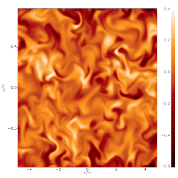
Figure 12: Snapshots of $B_{y}$ in the $(x,z)$ plane at time $t=66$ in model 256Re12500Pm2. The structure of the flow and the typical length scale of the fluctuations are similar to that obtained in model STD128 in paper I (see the middle panel of figure 4 in paper I with which the present figure should be compared).

In this paper, we studied the effect of finite dissipation coefficients on the saturated level of MRI–driven MHD turbulence. One of the important aspect of our results is that MHD turbulence can only be sustained if the magnetic Prandtl number $Pm$ is larger than some critical value $Pm_{c}$. For the limited range of Reynolds numbers that could be probed given current day limitations in computing time, we found that $Pm_{c}>1$. We want to stress here that these results are consistent with the results we obtained in paper I. Indeed, we argued in section 5.1 of that paper that it is possible to derive a “numerical” magnetic Prandtl number when using ZEUS without explicit diffusion coefficients and estimated its value, although very uncertain, to be of order unity and probably somewhat larger than one. The fact that MHD turbulence was found to be sustained in these simulations is therefore consistent with the results of the present paper, for which all of our “alive” case have $Pm$ larger than unity. If ZEUS had had a numerical magnetic Prandtl number smaller than unity, we would predict from the present result that MHD turbulence would decay when performing such simulations without explicit dissipation coefficients.

It is in fact possible to push the comparison between the results of paper I and paper II a bit further. Indeed, we note that model STD128 (presented in paper I) and model 256Re12500Pm2 (presented in this paper) have similar time averaged value of $\alpha$: $2.2\times 10^{-3}$ for the former and $1.6\times 10^{-3}$ for the later. This similar result is due to the fact that both model lie in the same region of the $(Re,Pm)$ plane: for model 256Re12500Pm2, $Re_{M}=25000$ and $Pm=2$. For model STD128, we estimated in paper I that $Re_{M}$ is of the order of $30000$ while $Pm$ is of the order or slightly larger than one. This is why the results are similar. This is further illustrated on figure 12 which shows a snapshot of $B_{y}$ at time $t=66$ in model 256Re12500Pm2. Note how similar it is to the middle panel of figure 4 in paper I, which shows the same variable for model STD128. Measuring the typical length scale $L_{y}(B_{y})$ of the magnetic structures in model 256Re12500Pm2 using Eq. (9) of paper I, we found a time averaged value $L_{y}(B_{y})=0.045$, very close to the value $0.04$ we obtained for model STD128.

It is also possible to compare the results of model STD64 of paper I to the results of the present paper. We recall here that we found the rate of angular momentum transfer in this model to be such that $\alpha\sim 0.004$ when time averaged over the simulation. For model STD64, we estimated in paper I that $Re_{M}\sim 10^{4}$ and a similar value for the magnetic Prandtl number as for model STD128. This would correspond to Reynolds number somewhat smaller than $10000$. In the present paper, we found that $\alpha\sim 0.01$ for model 128Re3125Pm4, for which $Re=3125$ and $Pm=4$, while model 128Re3125Pm2, having $Re=3125$ and $Pm=2$ was shown to decay. It is therefore tempting to identify model STD64 with a model that would be intermediate between the last two cases. Using the PENCIL code, we ran such a model, having $Re=3125$ and $Pm=3$, and found $\alpha=0.007$ which is close to the result of model STD64.

We want to stress, however, that it would be dangerous to push such comparisons further than that. Indeed, we demonstrated in paper I that numerical dissipation generally departs from a pure Laplacian dissipation in ZEUS. Moreover, we stressed in paper I that an accurate estimate for the magnetic Prandtl number is difficult to obtain for a given simulation, as it depends on the nature of the flow itself. A one to one comparison between the results of paper I and paper II is therefore difficult to carry and may not bear much significance.

5.2 Small scales

The results of this paper together with paper I indicate the importance of flow phenomena occurring at the smallest scales available in a simulation, at least at currently feasible resolutions. In fact the importance of small scales determined by the transport coefficients is not unexpected when one considers previous work on the maintenance of a kinematic magnetic dynamo.

Although a kinematic dynamo considers only the induction equation with an imposed velocity field, some issues arising in that case may be relevant, especially if one wishes to consider the likely behaviour of turbulence driven by the MRI when the transport coefficients are reduced to very small values.

If a dynamo is to be maintained in a domain such as a shearing box with no net flux, one would expect that the magnitude of a magnetic field could be amplified from a small value through the action of some realised velocity field. Furthermore if such an amplification occurs within a specified time scale and for arbitrarily small resistivity, it would be classified as a fast dynamo. In the special case when the imposed velocity field is stationary Moffatt & Proctor (1985) have shown that the field produced by such a dynamo must have a small spatial scale determined by the resistivity. A well known example of this type is generated by the so called ’ABC’ flow (see Teyssier et al. 2006, and references therein). This example also shows that certain quantities such has the growth rate of the dynamo do not have a simple dependence on magnetic Reynolds number when that is relatively small and thus caution should be exercised in making any simple extrapolation.

Although the case of a steady state velocity field is rather special, the result can be very easily seen to hold more generally for the case when the magnetic field is presumed to have net helicity. The magnetic helicity ${\cal H},$ which may be regarded as a topological quantity measuring the degree of entanglement or knottedness of the field, is defined by

$${\cal H}=\int_{V}\mbox{\boldmath{$A$}}\cdot\mbox{\boldmath{$B$}}dV,$$ (9)

where ${\bf A}$ is the vector potential and the integral is over the whole box. In our case the boundary conditions ensure ${\cal H}$ is gauge invariant. In ideal MHD ${\cal H}$ is conserved and so cannot grow by dynamo action. When the resistivity is non zero, the induction equation implies that (Moffatt & Proctor 1985)

$${d{\cal H}\over dt}=-2\int_{V}\eta(\nabla\times{\bf A})\cdot(\nabla\times{\bf B})dV.$$ (10)

Using the Schwartz inequality, this implies that

$$\left|{1\over{\cal H}}{d{\cal H}\over dt}\right|\leq 2\eta_{max}|{\cal K}|l^{-2},$$ (11)

where $\eta_{max}$ is the maximum value of $\eta,$ ${\cal K}$ is the inverse of the relative helicity given by

$${\cal K}=\sqrt{\int_{V}{\bf A}^{2}dV\int_{V}{\bf B}^{2}dV}/{\cal H}$$ (12)

and the length scale $l$ is defined through

$$l^{-4}={\int_{V}|\nabla\times{\bf A}|^{2}dV\int_{V}|\nabla\times{\bf B}|^{2}dV\over\int_{V}{\bf A}^{2}dV\int_{V}{\bf B}^{2}dV}.$$ (13)

From equation (10) one can argue that for any field with non zero relative helicity to grow in a finite time, the scale length $l$ must decrease to arbitrarily small scales as the transport coefficients are decreased to small values.

Although the above problems are not directly dealing with the MRI, and the discussion is by no means comprehensive, it is suggestive in indicating that significant flow structures plausibly occur at small scales as the transport coefficients are decreased and also that some features may not vary monotonically as a function of Reynolds number.

Another important feature apparent in the results presented here is the increase of turbulent activity with Prandtl number at fixed Reynolds number. This is difficult to quantify but may be connected to the increasing inhibition of reconnection by moving field lines together when the viscosity increases.

In this context it is important to emphasize that the simulations discussed here were carried out using an isothermal equation of state. However, there can be situations where a thermal diffusivity needs to be considered in addition to viscosity and resistivity. The isothermal approximation should be reasonable as long as any length scale introduce by heat diffusion is significantly longer than the resistive or viscous scales. When this length scale becomes comparable to the others we would expect the velocity and pressure fields to be affected on this scale. This too may affect reconnection rates, the operation of a small scale dynamo and a consequent inverse cascade. But the necessity of small scales as argued above depends on a balance determined by the induction equation and is not affected.

5.3 Towards an asymptotic regime for the zero net flux shearing box

Figure 13: Cartoon showing the variation of the critical Prandtl number $Pm_{c}$, above which MHD turbulence is sustained as a function of the Reynolds number. As simulations have not attained an asymptotic regime, qualitative changes of behaviour cannot be ruled out if $Re$ were to be increased further.

As we mentioned above, we have demonstrated in the present paper that for each value of the Reynolds number, there exists a critical Prandtl number $Pm_{c}$ below which turbulence decays. The variation of $Pm_{c}$ with $Re$ is sketched on figure 13. Given this plot, one may want to extrapolate the behaviour of $Pm_{c}$ at large $Re$. We want to stress that such an extrapolation cannot be made based on our results: we did not reach an asymptotic regime within the parameter regime we were able to study. This will require further simulations, performed at larger Reynolds number. Such calculations will have to be performed at resolutions $(512,800,512)$ and higher and will be extremely demanding computationally. At the present time, any of the following behaviour should be considered possible: $Pm_{c}$ could monotonically decrease to zero, tend to a finite value or reach a minimum increasing again for larger $Re$.

However, it is interesting to note in this context that recent work on fluctuating dynamos (driven by external forcing) indicate that they can be maintained at small $Pm$ but increasing values of $Re$ are required as this decreases (Boldyrev & Cattaneo 2004; Ponty et al. 2005; Iskakov et al. 2007) exacly as one would extrapolate using Figure 13. We also point out that these results, as do those based on kinematic dynamos, indicate the importance of dynamo generated fields on small scales and also that these may in turn act as a source for field on larger scales. Clearly simulations at much higher resolution are required to investigate the existence of such a regime in our case.

Another question that cannot be answered yet is whether $\alpha$ attains a finite limit at large Reynolds number for a given Prandtl number. The answer to this question would also require the resolution to be increased in order to extend the domain that can be probed in the $(Re,Pm)$ plane. Both issues are astrophysically important and need to be addressed in the future as soon as the computing resources become more readily accessible to the community.

5.4 Future work

It is also important to stress that the work in this paper applies to an extremely simple set up of an unstratified shearing box with zero net flux. The reason for focusing on this case was that it has been considered that it could offer the possibility of a dynamo in the local limit, this being independent of exterior boundary conditions and imposed magnetic fields.

The work here indicates the possibility of the importance of small scales and only modest angular momentum transport in this limit. It therefore also emphasises the need for studies of more general configurations which take account of stratification, global boundary conditions and imposed fields. There is no reason to suppose that consideration of transport coefficients and small scale phenomena are not important in these cases also so this should be an important area for future investigations.

References

- Balbus & Hawley (1998) Balbus, S. & Hawley, J. 1998, Rev.Mod.Phys., 70, 1
- Boldyrev & Cattaneo (2004) Boldyrev, S. & Cattaneo, F. 2004, Physical Review Letters, 92, 144501
- Brandenburg & Dobler (2002) Brandenburg, A. & Dobler, W. 2002, Computer Physics Communications, 147, 471
- Fleming et al. (2000) Fleming, T. P., Stone, J. M., & Hawley, J. F. 2000, ApJ, 530, 464
- Fromang & Papaloizou (2006) Fromang, S. & Papaloizou, J. 2006, A&A, 452, 751
- Fromang & Papaloizou (2007) Fromang, S. & Papaloizou, J. C. B. 2007, A&A, submitted
- Goldreich & Lynden-Bell (1965) Goldreich, P. & Lynden-Bell, D. 1965, MNRAS, 130, 125
- Hawley & Stone (1995) Hawley, J. & Stone, J. 1995, Comput. Phys. Commun., 89, 127
- Hawley et al. (1995) Hawley, J. F., Gammie, C. F., & Balbus, S. A. 1995, ApJ, 440, 742
- Hawley et al. (1996) Hawley, J. F., Gammie, C. F., & Balbus, S. A. 1996, ApJ, 464, 690
- Iskakov et al. (2007) Iskakov, A., Schekochihin, A., Cowley, S., McWilliams, J. C., & Proctor, M. R. E. 2007, Physical Review Letters, 98, 208501
- Landau & Lifshitz (1959) Landau, L. D. & Lifshitz, E. M. 1959, Fluid mechanics (Course of theoretical physics, Oxford: Pergamon Press, 1959)
- Lesur & Longaretti (2005) Lesur, G. & Longaretti, P.-Y. 2005, A&A, 444, 25
- Lesur & Longaretti (2007) Lesur, G. & Longaretti, P.-Y. 2007, MNRAS, 378, 1471
- Moffatt & Proctor (1985) Moffatt, H. K. & Proctor, M. R. E. 1985, JFM, 154, 493
- Papaloizou et al. (2004) Papaloizou, J. C. B., Nelson, R. P., & Snellgrove, M. D. 2004, MNRAS, 350, 829
- Ponty et al. (2005) Ponty, Y., Mininni, P., Montgomery, D., Pinton, J.-F. Politano, H., & Pouquet, A. 2005, Physical Review Letters, 94, 164502
- Sano et al. (2004) Sano, T., Inutsuka, S., Turner, N. J., & Stone, J. M. 2004, ApJ, 605, 321
- Schekochihin et al. (2004) Schekochihin, A. A., Cowley, S. C., Taylor, S. F., Maron, J. L., & McWilliams, J. C. 2004, ApJ, 612, 276
- Teyssier et al. (2006) Teyssier, R., Fromang, S., & Dormy, E. 2006, Journal of Computational Physics, 218, 44
- Umurhan & Regev (2004) Umurhan, O. M. & Regev, O. 2004, A&A, 427, 855
- Ziegler & Yorke (1997) Ziegler, U. & Yorke, H. W. 1997, Computer Physics Communications, 101, 54