MHD simulations of the magnetorotational instability in a shearing box with zero net flux. I. The issue of convergence

Abstract

Aims. We study the properties of MHD turbulence driven by the magnetorotational instability (MRI) in accretion disks. To do this we perform a series of numerical simulations for which the resolution is gradually increased.

Methods. We adopt the local shearing box model and focus on the special case for which the initial magnetic flux threading the disk vanishes. We employ the finite difference code ZEUS to evolve the ideal MHD equations.

Results. Performing a set of numerical simulations in a fixed computational domain with increasing resolution, we demonstrate that turbulent activity decreases as resolution increases. The highest resolution considered is $256$ grid cells per scale height. We quantify the turbulent activity by measuring the rate of angular momentum transport through evaluating the standard $\alpha$ parameter. We find $\alpha=0.004$ when $(N_{x},N_{y},N_{z})=(64,100,64)$, $\alpha=0.002$ when $(N_{x},N_{y},N_{z})=(128,200,128)$ and $\alpha=0.001$ when $(N_{x},N_{y},N_{z})=(256,400,256)$. This steady decline is an indication that numerical dissipation, occurring at the grid scale is an important determinant of the saturated form of the MHD turbulence. Analysing the results in Fourier space, we demonstrate that this is due to the MRI forcing significant flow energy all the way down to the grid dissipation scale. We also use our results to study the properties of the numerical dissipation in ZEUS. Its amplitude is characterised by the magnitude of an effective magnetic Reynolds number $Re_{M}$ which increases from $10^{4}$ to $10^{5}$ as the number of grid points is increased from $64$ to $256$ per scale height.

Conclusions. The simulations we have carried out do not produce results that are independent of the numerical dissipation scale, even at the highest resolution studied. Thus it is important to use physical dissipation, both viscous and resistive, and to quantify contributions from numerical effects, when performing numerical simulations of MHD turbulence with zero net flux in accretion disks at the resolutions normally considered.

1 Introduction

A long standing issue in accretion disk theory has been to identify the source of anomalous transport of angular momentum. To date, the most likely mechanism is believed to be the magnetorotational instability (MRI; Balbus & Hawley 1998) which simply requires a weak magnetic field and a radially decreasing angular velocity to operate in a highly conducting disk. Appropriate conditions are readily realised in many astrophysical accretion disks and the linear instability grows on dynamical timescales. Its nonlinear evolution has been widely studied since the early 1990’s. Local simulations using the shearing box model (Hawley et al. 1995; Brandenburg et al. 1995) were found to give rise to MHD turbulence with an associated rate of angular momentum transport compatible with the observations, with $\alpha$, the standard parameter in standard disk theory (Shakura & Sunyaev 1973), being in the range $10^{-3}$–$0.1$ depending on the geometry of the magnetic field.

In this paper we focus on MHD simulations in a shearing box threaded by zero net magnetic flux initially and use the operator split code ZEUS (Hawley & Stone 1995). The first detailed consideration of this case was by Hawley et al. (1996). The potential importance for angular momentum transport in accretion disks is that it offers the possibility of local turbulence coupled with genuine dynamo action. If such activity can be maintained, it would be independent of any imposed magnetic field and being local, independent of distant boundary conditions. Accordingly this would be a robust outcome of the MRI, providing a guaranteed level of transport. However, some recent results (Gardiner & Stone 2005b) indicate that the saturated turbulent state is sensitive to numerical resolution. Accordingly, issues remain as to whether a numerically converged saturated turbulent state can be achieved. It is important to note that should such simulations ultimately yield negligible or zero transport, the MRI can still operate to produce sustained turbulence and transport, but more attention would have to be paid to imposed fields and boundary conditions in the context of global simulations which have been and are being currently carried out (Hawley 2001; Steinacker & Papaloizou 2002; Fromang & Nelson 2006).

The plan of the paper is as follows: In section 2 we describe the computational set up for the simulations we performed and algorithm used. We then go on to present results for typical runs. In section 3 we discuss the effect of resolution on the results and in section 4 we discuss the power spectra associated with the saturated turbulent states and use these to show that significant flow energy is always driven to the smallest numerically realisable scales. Thus results remain dependent on resolution at the highest resolution studied. We then go on to discuss these results and their implications for understanding the non linear outcome of the MRI in section 5 and give our conclusions in section 6.

2 Initial conditions and run setup

In this paper we solve the ideal MHD equations in a shearing box (Goldreich & Lynden-Bell 1965) using ZEUS (Hawley & Stone 1995). To do this we adopt a Cartesian coordinate system $(x,y,z)$ with unit vectors $(\mbox{\boldmath{$i$}},\mbox{\boldmath{$j$}},\mbox{\boldmath{$k$}})$ pointing in the directions of the coordinate axes. The vertical direction is defined by $k$ and the azimuthal direction by $\mbox{\boldmath{$j$}}.$ The frame rotates with the angular velocity of a free particle in circular orbit at the centre of the box and the origin of the coordinate system $\mbox{\boldmath{$\Omega$}}=\Omega\mbox{\boldmath{$k$}}$. In this frame the basic equations can be written as

$$\frac{\partial\rho}{\partial t}+\mbox{\boldmath{$\nabla$}}\mbox{\boldmath{$\cdot$}}(\rho\mbox{\boldmath{$v$}}) = 0\,,$$ (1)

$$\rho\frac{\partial\mbox{\boldmath{$v$}}}{\partial t}+\rho(\mbox{\boldmath{$v$}}\mbox{\boldmath{$\cdot$}}\mbox{\boldmath{$\nabla$}})\mbox{\boldmath{$v$}}+2\rho\mbox{\boldmath{$\Omega$}}\times\mbox{\boldmath{$v$}} = -\mbox{\boldmath{$\nabla$}}P+\frac{1}{4\pi}(\mbox{\boldmath{$\nabla$}}\mbox{\boldmath{$\times$}}\mbox{\boldmath{$B$}})\mbox{\boldmath{$\times$}}\mbox{\boldmath{$B$}},$$ (2)

$$\frac{\partial\mbox{\boldmath{$B$}}}{\partial t} = \mbox{\boldmath{$\nabla$}}\mbox{\boldmath{$\times$}}(\mbox{\boldmath{$v$}}\mbox{\boldmath{$\times$}}\mbox{\boldmath{$B$}})\,.$$ (3)

Here $\rho$ stands for the gas density, $v$ for the velocity, $B$ for the magnetic field and $P$ for the pressure.

To close the system written above, one need to specify the pressure through an equation of state. For reasons of simplicity, throughout this paper we adopt an isothermal equation of state for which

$$P=\rho c_{0}^{2}\,.$$ (4)

As usual, the ratio between the speed of sound $c_{0}$ and the angular frequency $\Omega$ can be used to define a disk scale height $H$.

Given the above framework, a simulation is defined once the size of the box, the resolution and the initial geometry and strength of the magnetic field are chosen. In this paper, for the most part, we consider computational boxes of size $(L_{x},L_{y},L_{z})\equiv(H,\pi H,H)$, although we have also considered boxes of size $(H,2\pi H,H)$ in order to compare our simulations with those published in the literature previously. The resolutions used vary from $(N_{x},N_{y},N_{z})=(64,100,64)$ to $(N_{x},N_{y},N_{z})=(256,400,256)$. We will measure times in units of the orbital period, $T=2\pi/\Omega$. As mentioned in the introduction, we focus exclusively on the special case in which no net magnetic flux threads the box (in the vertical or azimuthal directions) initially. The magnetic field at the start of the simulation is purely vertical and defined as follows:

$$B_{z}=B_{0}\sin(2\pi x/H)$$ (5)

where $B_{0}$ is set such that the volume average ratio between thermal and magnetic pressure $<\beta>$ equals $400$. We checked, however, that the saturated state of the turbulence depends neither on that value nor on the geometry of the field provided the net flux remains zero. At the beginning of each simulations, random velocity fluctuations of small amplitude are applied to an initial state with uniform gas density and velocity that is entirely due to the background Keplerian shear and takes the form $\mbox{\boldmath{$v$}}=(0,-3\Omega x/2,0).$ All the simulations performed here had the Courant number $C=1/2.$

Following standard practise (Hawley et al. 1995) strictly periodic boundary conditions are applied in $y$ and $z$ while boundary conditions that are periodic in shearing coordinates are applied in $x$. The latter require some care as they might introduce spurious numerical artefacts. Here, we applied these shearing box boundary conditions directly to the magnetic field. Although this procedure safely conserves the mean radial magnetic field threading the box to within round–off error, the mean y and z components of the field are only conserved to within truncation error. Thus there is a possibility of having long term accumulation of azimuthal or vertical magnetic fluxes, which would increase the MRI–induced turbulent activity in the box. In the following, we will therefore monitor the time variation of the mean y and z components threading the computational domain during the simulations.

2.1 Run parameters

Model	Box size	Resolution	Run time (in orbits)	$\alpha_{Rey}$	$\alpha_{Max}$	$\alpha$
FS64	$(H,2\pi H,H)$	$(64,200,64)$	$300$	$1.8\times 10^{-3}$	$4.2\times 10^{-3}$	$5.9\times 10^{-3}$
STD64	$(H,\pi H,H)$	$(64,100,64)$	$1000$	$9.4\times 10^{-4}$	$3.2\times 10^{-3}$	$4.1\times 10^{-3}$
STD128	$(H,\pi H,H)$	$(128,200,128)$	$250$	$5.0\times 10^{-4}$	$1.7\times 10^{-3}$	$2.2\times 10^{-3}$
STD256	$(H,\pi H,H)$	$(256,400,256)$	$105$	$2.4\times 10^{-4}$	$8.1\times 10^{-4}$	$1.1\times 10^{-3}$
STD64a	$(H/2,\pi H/2,H/2)$	$(64,100,64)$	$120$	$3.3\times 10^{-4}$	$1.4\times 10^{-3}$	$1.7\times 10^{-3}$
LB64	$(2H,2\pi H,H)$	$(128,200,64)$	$120$	$1.5\times 10^{-3}$	$3.6\times 10^{-3}$	$5.2\times 10^{-3}$
LB128	$(2H,2\pi H,H)$	$(256,400,64)$	$105$	$8.3\times 10^{-4}$	$2.1\times 10^{-3}$	$2.8\times 10^{-3}$

Table 1: Properties of the runs described in this paper: The first column gives the model label, while the next three columns give the size of the computational domain $(L_{x},L_{y},L_{z}),$ the resolution $(N_{x},N_{y},N_{z})$ and the time (in orbits) for which the simulation was run respectively. The fifth to seventh columns indicate the rate of angular momentum transport by giving the volume and time averaged value of the Reynolds, Maxwell and total stresses, normalised by the initial thermal pressure, respectively (note that these values are obtained in each case by averaging the results from $t=40$ orbits until the end of the simulation).

The details of the runs we performed are given in Table 1. The first column gives the simulation label. The second and third column give the box dimensions $(L_{x},L_{y},L_{z})$ and the resolution $(N_{x},N_{y},N_{z}).$ The fourth column gives the simulation duration in orbital times. Finally, the last three columns give time averaged values of the Reynolds, Maxwell and total stresses, normalised by the initial thermal pressure $P_{0}$. They measure the rate of angular momentum transport and as usual are respectively defined through

$$\alpha_{Rey} = \frac{T_{r\phi}^{Rey}}{P_{0}}=\frac{1}{P_{0}}\langle\rho(v_{x}-\bar{v_{x}})(v_{y}-\bar{v_{y}})\rangle\,,$$ (6)

$$\alpha_{Max} = \frac{T_{r\phi}^{Max}}{P_{0}}=\frac{1}{P_{0}}\left\langle-{B_{x}B_{y}\over 4\pi}\right\rangle\,,$$ (7)

$$\alpha = \alpha_{Rey}+\alpha_{Max}=\frac{T_{r\phi}^{Max}+T_{r\phi}^{Rey}}{P_{0}}\,.$$ (8)

In these equations, ${\overline{v}_{x}}$ and ${\overline{v}_{y}}$ are averages over $y$ and $z$ of the velocity components in the $x$ and $y$ directions respectively while the angled brackets denote a volume average. Note that because of the conservation of mass $P_{0}=\langle P\rangle.$

2.2 Standard runs

Figure 1: Time history of the stress parameters $\alpha_{Rey}$, $\alpha_{Max}$ and $\alpha$ for the runs FS64 (upper panel) and STD64 (lower panel). For each plot, the dotted curve corresponds to the Reynolds stress, the dashed curve corresponds to the Maxwell stress while the solid curve is the sum of the two. All of these are normalised by the initial thermal pressure.

To make a connection with previously published results, we first perform two runs with a moderate resolution. Both have $64$ grid cells in the $x$ and $z$ direction. The first, labelled FS64, uses a box size $(L_{x},L_{y},L_{z})=(H,2\pi H,H)$ and $200$ cells in the y direction. It is almost identical to one of the runs presented by Fleming et al. (2000). The only difference is that these authors use an adiabatic equation of state and a somewhat lower resolution in the $y$ direction. Model FS64 is compared with model STD64 in which the size of the computational box is halved in the $y$ direction. To maintain the same effective resolution, $N_{y}$ is also decreased to $100$. Thanks to the improved computational resources that have become available in the last few years, models FS64 and STD64 have been run for $300$ and $1000$ orbits respectively.

The time history of $\alpha_{Rey}$, $\alpha_{Max}$ and $\alpha$ are shown for both runs FS64 and STD64 in figure 1 respectively on the upper and lower panels. In each case, the dotted line represents $\alpha_{Rey}$, the dashed line shows $\alpha_{Max}$ while the solid line corresponds to $\alpha$, the sum of the two. Both runs display the characteristic signatures of the MRI: an initial growth during the first few orbits due to the linear instability, a decrease of the stress after reaching a maximum as the linear instability breaks down into MHD turbulence and finally attainment of a saturated quasi steady state phase characterised by outward angular momentum transport for the remainder of the simulation. As observed in most simulations of this type, most of the transport is due to the contribution of the Maxwell stress. Both runs show sustained MHD turbulence for hundreds of orbits, in agreement with earlier studies (Sano et al. 2004), with significant fluctuations occurring on both short (less than $1$ orbit) and long timescales (more than $10$ orbits). Time–averaged values of the stresses between $t=40$ and the end of the simulation, are given for both runs in Table 1. For model FS64, we find values almost identical to those reported by Fleming & Stone (2003) in their Table 2. For model STD64, we find that the transport is weaker by about $30\%$, as for this model $\alpha=4.1\times 10^{-3}$ whereas $\alpha=5.9\times 10^{-3}$ in model FS64. The difference is due to the smaller box size in model STD64, as this is the only difference between the two simulations. Although this relation between the box size and turbulent activity is not yet well understood, it was already noted in earlier calculations of the shearing box (Hawley et al. 1996).

In conclusion, models FS64 and STD64 demonstrate good agreement between our results and previously published calculations. The next step, which is the main goal of this paper, is to check the convergence of these results when resolution is increased. Given the large computational cost associated with well resolved simulations, it is necessary to choose one particular box size for these runs despite the differences between the runs FS64 and STD64 mentioned above. To reduce the computational burden, we adopt the smaller box for the remainder of this paper, as the computing time is reduced by a factor of two. The consequences of changing the box size will be briefly considered in section 5.2.

3 The effect of resolution

Figure 2: Same as figure 1 but for the runs STD128 (upper panel) and STD256 (lower panel). Note the overall decreasing turbulent activity as the resolution is increased.

Figure 3: Time history of the mean azimuthal (solid line) and vertical (dashed line) magnetic field threading the box in model STD128, normalised by $P_{0}^{1/2}$. Both remain small enough no to affect the long term evolution of the simulations.

In this section, we study the influence of resolution on the results of model STD64 by doubling (model STD128) and quadrupling (model STD256) the number of cells in each coordinate direction. All other parameters are kept identical to those of STD64. The time history of the normalised stresses is shown in figure 2 for models STD128 and STD256 in the upper and lower panels (using the same conventions as in figure 1) respectively. It is clear from figure 2 that $\alpha_{Max}$ and $\alpha_{Rey}$ both decrease as resolution is increased. From Table 1, the time averaged value of $\alpha$ in model STD128 is $2.2\times 10^{-3}$ while it is $1.1\times 10^{-3}$ in model STD256. In other words, in going from $64$ grid points to $256$ grids points per scale height, the turbulent activity decreases by approximately a factor of two each time the resolution increases by a factor of $2$. Figure 2 also shows that the amplitude of the fluctuations of the stresses tends to decrease as the resolution is increased. This could be a signature of the decreasing importance of channel flows that have been suggested as being responsible for these fluctuations (Sano 2007), as resolution is increased.

Model STD256 is run for $105$ orbits. The lower resolution models STD64 and STD128 show that this is enough to get a good estimate of the stresses. Indeed, averaging $\alpha$ in these two models between $t=40$ and $t=105$, we respectively found $\alpha=4.3\times 10^{-3}$ and $2.5\times 10^{-3}$, which are close to the values quoted in Table 1 and obtained by averaging over much longer periods. Averaging the stresses over $105$ orbits should therefore be enough to get a good estimate of $\alpha$.

Next, we turn our attention to possible problems induced by the shearing box boundary conditions. To check whether y and z mean magnetic field are created in the box, we plot in figure 3 the time history of both in model STD128, normalised by $P_{0}^{1/2}$. It shows no systematic increasing accumulation of net flux in the computational domain, despite the imperfect nature of the shearing box boundary conditions. Furthermore, the absolute value of both components is always very small. Their maximum strength during the simulation, expressed in terms of effective beta values (defined as $\beta_{i}=8\pi P_{0}/\!<\!\!B_{i}\!\!>^{2}$), is respectively $\beta_{y}=5.4\times 10^{6}$ and $\beta_{z}=4.3\times 10^{6}$ for the y and z components. For the resolution we are using, this is far too small a field strength to have any effect on the saturated state of the turbulence (the wavelength of the most unstable MRI mode for such weak fields is always smaller than a grid cell). We performed the same checks for models STD64 and STD256. For the former, the maximum values of the mean field components during the simulations corresponded to $\beta_{y}=2.3\times 10^{6}$ and $\beta_{z}=1.5\times 10^{7}$. For the later, we obtained $\beta_{y}=3.8\times 10^{8}$ and $\beta_{z}=1.7\times 10^{8}$. All these values indicate that the boundary conditions have no effect on the results.

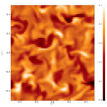
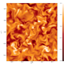
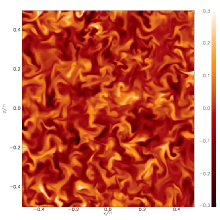
Figure 4: Snapshots showing contours of the y–component of the magnetic field in the $(x,z)$ plane $(y=0)$ for the runs STD64 (left panel), STD128 (middle panel) and STD256 (right panel). Smaller and smaller scale features in the magnetic field are seen as the resolution of the simulation increases.

Figure 5: Time history of the correlation length in the $z$ direction of $B_{y}$ for models STD64 (solid line), STD128 (dashed line) and STD256 (dotted line). As the resolution is increased, $L_{z}(B_{y})$ decreases, as might be expected from the appearance of the snapshots shown in figure 4.

Being confident that the models we present are not significantly affected by the boundary conditions, we now turn to a more detailed analysis of their properties. To illustrate the changes in the structure of the flow as resolution is increased, figure 4 provides snapshots of the structure of the magnetic field. From left to right, contours of $B_{y}$ in the $(x,z)$ plane $(y=0)$ are given for models STD64 (left panel), STD128 (middle panel) and STD256 (right panel). As the resolution is increased, smaller and smaller scale structure becomes apparent. The only limitation on the smallness of the scale appears to be due to finite resolution. It is possible to make this statement more quantitative by computing a vertical correlation length for $B_{y}$. Following Lesur & Longaretti (2007), we define this correlation length through

$$L_{z}(B_{y})=\left<\frac{\int\int B_{y}(x,y=0,z)B_{y}(x,y=0,z^{\prime})dz^{\prime}dz}{\int B_{y}^{2}(x,y=0,z)dz}\right>\,.$$ (9)

In this definition, the symbol angled brackets denote an average over the $x$ direction. The time history of $L_{z}(B_{y})$ is plotted in figure 5, using a solid line for model STD64, a dashed line for model STD128 and a dotted line for model STD256. Because the raw data were very noisy, the initial curves were smoothed using a window of about $3$ orbits, corresponding to $10$ snapshots. Figure 5 confirms the contraction of scale apparent from the trends seen in figure 4: after about $40$ orbits, $L_{z}(B_{y})$ reaches a quasi steady value which decreases as resolution is increased. Averaging the results in time from $t=40$ orbits until the end of the run, we obtained $L_{z}(B_{y})/H=0.06$ for model STD64, $0.04$ for model STD128 and $0.025$ for model STD256. For each model, these numbers indicate that typical size scale for structures in $B_{y}$ is a few grid cells. For model STD64, $L_{z}(B_{y})$ corresponds to $3.8$ grid cells, while it is equal to $5$ grid cells for model STD128 and $6.5$ grid cells for model STD256. Similar values are obtained when calculating a correlation length in the direction $x$, defined using an equation similar to Eq. (9).

All of these results indicate that the saturated state of MHD turbulence in these simulations is governed by the numerical dissipation of the code. It is therefore important to understand in a more detailed way the dissipation in ZEUS (and by extension any MHD code without specified diffusivities that relies on numerical dissipation to bound the size scale from below) and why and how it affects the results. In the following section, we use Fourier analysis to address this issue.

4 Fourier analysis

4.1 Power spectra

Figure 6: Reduced power spectra of the kinetic energy (upper panel) and of the magnetic field (lower panel) in the z–direction. On both plots, the solid line corresponds to model STD64, the dashed line to model STD128 and the dotted line to model STD256. The dot-dashed line on the upper panel shows the slope $k^{-11/3}$ expected in the standard Kolmogorov theory of incompressible hydrodynamic turbulence.In this and similar plots $k$ is expressed in units of $1/L$.

Useful clues into the nature of MHD turbulence are usually provided by power spectra. Here we compute the reduced power spectrum of kinetic energy in the vertical direction, which we define as

$$E(k_{z})=\frac{1}{2}\rho_{0}|\mbox{\boldmath{$\tilde{v}$}}(k_{z})|^{2}\,,$$ (10)

where $|\mbox{\boldmath{$\tilde{v}$}}(k_{z})|^{2}=|\tilde{v_{x}}(k_{z})|^{2}+|\tilde{v_{y}}(k_{z})|^{2}+|\tilde{v_{z}}(k_{z})|^{2}$. $\tilde{v_{x}}(k_{z})$ is defined by

$${\tilde{v_{x}}}(k_{z})=<\int_{z}v_{x}(x,y,z)e^{-ik_{z}z}dz>\,,$$ (11)

where $<.>$ stands for an average in the $x$ and $y$ directions. Similar definitions hold for $\tilde{v_{y}}(k_{z})$ and $\tilde{v_{z}}(k_{z})$. In writing Eq. (10), $\rho_{0}$ stands for the (conserved) mean density of the flow. Similar expressions can be written to compute the reduced power spectrum of magnetic energy.

Both spectra are represented in figure 6 as a function of $k_{z}$. The upper panel shows the kinetic energy spectrum and the lower panel the magnetic energy spectrum. In both panels, the results of model STD64 are shown using the solid line, those of model STD128 are plotted with the dashed line and the dotted line finally represents the results of model STD256. At all resolutions, both kinetic and magnetic energy spectra show features typical of turbulence: the spectrum decreases with $k_{z}$, showing that there is more energy at large scale. Note however the decreasing power at large scales (both for the kinetic and magnetic energies) as resolution is increased. This is because turbulent activity (or, equivalently, angular momentum transport) decreases when resolution increases and is in agreement with the result of section 3. In the upper panel, the dot–dashed line enables the results to be compared with the expected slope of a Kolmogorov spectrum: $E(k_{z})\propto k_{z}^{-11/3}$. There is no identifiable region with the expected Kolmogorov slope, that is maintained as the resolution is increased, that can be seen in the computed spectra, the best resolved calculation spanning almost two orders of magnitude in $k_{z}$. For both the kinetic and magnetic energies, the spectra consist of a flat part at large scale, which grows in size as resolution is increased, and a decreasing part probably governed by numerical dissipation. In fact, these spectra fail to show any sign of an inertial range building up as resolution is increased. But is there any reason to expect these simulations to show a clear inertial range? Probably not. Because of the MRI, the flow is a priori unstable at all realisable scales and forcing and input is therefore expected to occur all the way from the largest scale available in the box down to the smallest MRI unstable scales (set by numerical dissipation). At these scales a small scale dynamo may also operate and even transfer some energy back to larger scales (Brummell et al. 1998; Boldyrev et al. 2005; Ponty et al. 2005). Thus in our case there is no good reason to suppose that any region of Fourier space is expected to be exclusively transferring kinetic or magnetic energy downward to smaller scales, as would be required for an inertial range to be observed. To demonstrate this more clearly, we consider the properties of the Fourier transformed induction equation in the next section.

In this context we comment that a situation where the MRI leads to dynamo activity differs from those such as occur when hydrodynamic phenomena such as the Rayleigh Taylor instability or Kelvin-Helmholtz instability produce turbulence. In the case of the Rayleigh Taylor instability, the source of energy is confined to the largest scales. Even though there are small scale instabilities in the linear regime, in the non linear regime these are overwhelmed by the advection process that results in the production of even smaller scales where dissipation takes place (Chertkov 2003). In the case of the Kelvin-Helmholtz instability, the situation is similar with a source of instability occuring only at large scales when there is no dynamo action (Nepveu 1985; Ryu et al. 2000).

4.2 Equations

We consider Eq. (3) and decompose the velocity as the sum of the mean shear flow and the turbulent velocity field:

$$\mbox{\boldmath{$v$}}=\mbox{\boldmath{$V_{sh}$}}+\mbox{\boldmath{$v_{t}$}}$$ (12)

where the mean shear flow is simply the $y$ and $z$ average of the $y$ component of the velocity.

$$\mbox{\boldmath{$V_{sh}$}}(x)=V_{sh}\mbox{\boldmath{$j$}}={1\over L_{y}L_{z}}\int\int v_{y}(x,y,z)dydz$$ (13)

Using this decomposition, the right hand side of equation (3) can be expanded and written as the sum of five terms:

$$\frac{\partial\mbox{\boldmath{$B$}}}{\partial t}=-V_{sh}\frac{\partial\mbox{\boldmath{$B$}}}{\partial y}+B_{x}\frac{\partial V_{sh}}{\partial x}\mbox{\boldmath{$j$}}-(\mbox{\boldmath{$v_{t}$}}\cdot\mbox{\boldmath{$\nabla$}})\mbox{\boldmath{$B$}}-(\mbox{\boldmath{$\nabla$}}\cdot\mbox{\boldmath{$v_{t}$}})\mbox{\boldmath{$B$}}+(\mbox{\boldmath{$B$}}\cdot\mbox{\boldmath{$\nabla$}})\mbox{\boldmath{$v_{t}$}}$$ (14)

where the dependence of first two terms on velocity is through $V_{sh}$ only. These describe advection by the mean flow and stretching of the radial magnetic field lines by the background shear. We take the Fourier transform of this equation and dot the resulting equation with the complex conjugate of the Fourier transform of ${\mbox{\boldmath{$B$}}}.$ Denoting the later by $\tilde{\mbox{\boldmath{$B^{*}$}}}(\mbox{\boldmath{$k$}})$ and noting that

$${\tilde{\mbox{\boldmath{$B$}}}}(\mbox{\boldmath{$k$}})=\int\mbox{\boldmath{$B$}}(\mbox{\boldmath{$x$}})\exp{(-i\mbox{\boldmath{$k$}}\cdot\mbox{\boldmath{$x$}}})d^{3}{\mbox{\boldmath{$x$}}},$$ (15)

defines a finite Fourier transform, we obtain an equation governing the evolution of the magnetic energy density in Fourier space in the form

$$\frac{1}{2}\frac{\partial|\tilde{\mbox{\boldmath{$B$}}}(\mbox{\boldmath{$k$}})|^{2}}{\partial t}=A+S+T_{bb}+T_{divv}+T_{bv}\,,$$ (16)

where

$$A = -{\cal R}e\left[\tilde{\mbox{\boldmath{$B^{*}$}}}(\mbox{\boldmath{$k$}})\cdot\int\int\int V_{sh}\frac{\partial\mbox{\boldmath{$B$}}}{\partial y}e^{-i\mbox{\boldmath{$k$}}.\mbox{\boldmath{$x$}}}d^{3}\mbox{\boldmath{$x$}}\right]$$ (17)

$$S = +{\cal R}e\left[\tilde{B_{y}^{*}}(\mbox{\boldmath{$k$}})\cdot\int\int\int B_{x}\frac{\partial V_{sh}}{\partial x}e^{-i\mbox{\boldmath{$k$}}.\mbox{\boldmath{$x$}}}d^{3}\mbox{\boldmath{$x$}}\right]$$ (18)

$$T_{bb} = -{\cal R}e\left[\tilde{\mbox{\boldmath{$B^{*}$}}}(\mbox{\boldmath{$k$}})\cdot\int\int\int[(\mbox{\boldmath{$v_{t}$}}\cdot\mbox{\boldmath{$\nabla$}})\mbox{\boldmath{$B$}}]e^{-i\mbox{\boldmath{$k$}}.\mbox{\boldmath{$x$}}}d^{3}\mbox{\boldmath{$x$}}\right]$$ (19)

$$T_{divv} = -{\cal R}e\left[\tilde{\mbox{\boldmath{$B^{*}$}}}(\mbox{\boldmath{$k$}})\cdot\int\int\int(\mbox{\boldmath{$\nabla$}}\cdot\mbox{\boldmath{$v_{t}$}})\mbox{\boldmath{$B$}}e^{-i\mbox{\boldmath{$k$}}.\mbox{\boldmath{$x$}}}d^{3}\mbox{\boldmath{$x$}}\right]$$ (20)

$$T_{bv} = +{\cal R}e\left[\tilde{\mbox{\boldmath{$B^{*}$}}}(\mbox{\boldmath{$k$}})\cdot\int\int\int[(\mbox{\boldmath{$B$}}\cdot\mbox{\boldmath{$\nabla$}})\mbox{\boldmath{$v_{t}$}}]e^{-i\mbox{\boldmath{$k$}}.\mbox{\boldmath{$x$}}}d^{3}\mbox{\boldmath{$x$}}\right]\,$$ (21)

where ${\cal R}e$ denotes the real part is to be taken. Note that we applied the remap procedure described in Hawley et al. (1995) to account for the shear when computing the Fourier transform in the $x$ direction.

During the saturated phases of the previously described simulations, the time derivative of $|\tilde{\mbox{\boldmath{$B$}}}(\mbox{\boldmath{$k$}})|^{2}$ should vanish on average. In simulations of the MRI (Hawley et al. 1995; Brandenburg et al. 1995) it is quite generally found that quantities are stretched out in the direction of the shear and thus the length scales in the $x$ and $z$ direction associated with the saturated state are significantly smaller than the length scale in the $y$ direction. See for example Figure 4 of Hawley et al. (1995). Therefore we shall for simplicity consider only the particular Fourier plane defined by $k_{y}=0$ and then we get $A=0$. Under these assumptions, Eq. (16) simplifies to

$$S+T_{bb}+T_{divv}+T_{bv}=0\,.$$ (22)

In this equation, $S$ describes how the background shear creates the $y$ component of the magnetic field, $T_{bb}$ is a term that accounts for magnetic energy transfer toward smaller scales, $T_{divv}$ is due to compressibility and $T_{bv}$ describes how magnetic field is created due to field line stretching by the turbulent flow. Each of these terms now depends on the wavenumber $\mbox{\boldmath{$k$}}=(k_{x},k_{z})$. To improve the statistics, we average them on shell of given modulus $k=|\mbox{\boldmath{$k$}}|$ as well as over time.

Of course, in a real simulation of the type considered here, magnetic energy is damped by numerical dissipation. Therefore, a more realistic equation than Eq. (22) would be

$$S+T_{bb}+T_{divv}+T_{bv}+D_{num}=0\,.$$ (23)

where $D_{num}$ accounts for the numerical dissipation (of course ’realistic’ physical dissipation can be treated in a similar way, see paper II). In the following section, we study the balance between the various terms of Eq. (23) for models STD64, STD128 and STD256.

4.3 Results

Figure 7: Plots of the functions $S$ (solid line), $T_{bb}$ (dashed line), $T_{divv}$ (dotted line) and $T_{bv}$ (dotted–dashed line) as functions of $k$ for model STD256. These are averaged in time and Fourier space as described in the text. Note that $S$ is positive at all scales, which is simply describing the production of $B_{y}$ by the background shear.

Figure 8: Same as figure 7, but for the poloidal part of the magnetic energy. The term $T_{bv}^{P}$ is positive at all scales, indicating that MHD turbulence is forced by the MRI from the largest scale available in the simulation box down to the dissipative scale.

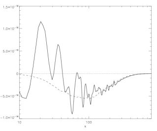
Figure 9: The solid line shows the variation of the numerical dissipation $D_{num}^{P}=-(T_{bb}^{P}+T_{divv}^{P}+T_{bv}^{P})$ with wavenumber $k$ for model STD256. It is compared, using the dashed line, with the spectrum $D_{res}$ that would result from a purely resistive dissipation corresponding to a magnetic Reynolds number $Re_{M}=10^{5}$ (see the text for the definition of $Re_{M}$). The thin solid line simply indicate the location of the zero on the plot. Note the good agreement between $D_{num}^{P}$ and $D_{res}$ at small scales, while they disagree significantly at large scales, showing that ZEUS numerical dissipation departs from a pure physical resistivity.

As model STD256 is the most detailed of our runs in term of resolution, we start by describing the results we obtained in this case before comparing with the other simulations. As mentioned above, the results of model STD256 were averaged in time to improve the statistics. We used $20$ dumps spanning about $60$ orbits from $t=45$ until the end of the simulation. Figure 7 plots the four terms appearing in Eq. (22) versus $k$. The solid, dashed, dotted and dotted–dashed lines respectively correspond to the terms $S$, $T_{bb}$, $T_{divv}$ and $T_{bv}$. Only the first is positive, while the other three terms are mainly negative, except for $T_{bb}$ which is positive at the largest scale of the box. The term $T_{divv}$, accounting for compressibility, is also seen to reach significant values, probably because of the presence a strongly nonlinear waves in these simulations (Gardiner & Stone 2005b; Papaloizou et al. 2004). The large and positive value of the $S$ term simply shows that $B_{y}$ is created at all scales by the background shear. For the MRI to be a proper dynamo, however, there has to be a way through which poloidal magnetic energy is regenerated from this toroidal field. To study that mechanism, we redo the analysis presented above but concentrate on the poloidal part of the magnetic field $\mbox{\boldmath{$B_{p}$}}=(B_{x},0,B_{z})$ rather than on the full magnetic field $B$. In that case, both $S$ and $A$ vanish and under the assumption that MHD turbulence is in steady state, Eq. (23) reduce to

$$T_{bb}^{P}+T_{divv}^{P}+T_{bv}^{P}+D_{num}^{P}=0\,,$$ (24)

where we have now

$$T_{bb}^{P}={\cal R}e\left[\tilde{\mbox{\boldmath{$B_{p}^{*}$}}}(\mbox{\boldmath{$k$}})\cdot\int_{x}\int_{y}\int_{z}(\mbox{\boldmath{$v_{t}$}}\cdot\mbox{\boldmath{$\nabla$}})\mbox{\boldmath{$B_{p}$}}e^{-i\mbox{\boldmath{$k$}}.\mbox{\boldmath{$x$}}}d^{3}\mbox{\boldmath{$x$}}\right]$$ (25)

with corresponding expressions for the other terms in Eq (24). The results we obtained for model STD256 are plotted on figure 8, with the same conventions as figure 7. They indicate that $T_{bv}^{P}$ is positive for all $k$ through turbulent velocity fluctuations creating poloidal magnetic field through field line stretching. $T_{bv}^{P}$ reaches its maximum at $k\sim 40$, which corresponds to roughly $1/8$th the size of the box (or $32$ grid cells at this resolution). Nevertheless there are non negligible contributions from the largest scale available in the box all the way down to $k\sim 200$, which corresponds to only a few grid cells. This is an indication that the MRI is forcing the flow at all available scales and explains why the power spectra presented in section 4.1 fail to show any inertial range.

Another application of the above analysis is to provide information about the dissipative properties of ZEUS. Indeed, because of Eq. (23), the sum of the three terms represented on figure 8 has to be balanced by the numerical dissipation. If that dissipation was exactly equivalent to a resistive process having a resistivity $\eta$, its spectrum $D_{res}(k)$ would be given by

$$D_{res}(k)=\eta k^{2}|\tilde{\mbox{\boldmath{$B_{p}$}}}(k)|^{2}\,.$$ (26)

In Figure 9 we plot $D_{num}^{P}$ (solid line) and $-D_{res}$ (dashed line). In the later case we chose $\eta$ in order to get a good fit between both curves. At large $k$ (or small scales), it is seen that $-D_{res}$ is in good agreement with $D_{num}^{P}$. This fit can be used to estimate the numerical resistivity $\eta$ of the code (at this particular resolution for small scales and for this specific flow). This translates into an effective magnetic Reynolds number $Re_{M}=c_{0}H/\eta$ which is of the order of $10^{5}.$ This equivalence has to be used with caution, however, as both $D_{num}^{P}$ and $-D_{res}$ deviate significantly for values of $k$ smaller than $80$. A contribution to this difference may arise from the poorer statistics available at the largest scale of the simulations (and particularly to non negligible contribution of the time derivative term in Eq. (16) at these scales), but it is also likely to be due to the fact that numerical dissipation cannot be simply described as arising from a diffusion process, at least at large scales. Also, it should be noted that the maximum amplitude of $D_{num}^{P}$ (and therefore the location where most of the dissipation takes place) occurs at $k\sim 70$–$100$, at which point the term $T_{bv}^{P}$ is still very significant (see figure 8). This is why the saturated state of MRI driven MHD turbulence depends on resolution. Based on this analysis, we would therefore predict that increasing the resolution by another factor of two would give a different saturated rate of angular momentum transport.

Figure 10: The left panel is the same as figure 8, but computed using results of model STD64. Likewise, the right panel is the same as figure 9 applied to model STD64. The dashed line use a resistivity $\eta$ such that $Re_{M}=10^{4}$.

Figure 11: Same as figure 10, but for model STD128. On the right panel, the value of $\eta$ used to fit the numerical results is such that $Re_{M}=3\times 10^{4}$.

In order to further investigate the effect of resolution, we repeated the previous analysis for models STD64 and STD128. For model STD64, we used about $90$ dumps regularly spaced in time during the $1000$ orbits of the simulations to average the results. For model STD128, we used $60$ dumps that cover the last $200$ orbits of the simulations. The results are summarised in figures 10 and 11 respectively. On both figures, the left panel is the equivalent of figure 8. These confirm the results obtained using model STD256. The MRI forces the flow at all available scales in the computational box. The right panels of figures 10 and 11 are equivalent to figure 9 but for models STD64 and STD128 respectively. Both confirm that small scale dissipation in ZEUS is similar to that provided by a physical resistivity, with magnetic Reynolds numbers of the order of $10^{4}$ and $3\times 10^{4}$ respectively. However, as also seen for model STD256, numerical resistivity departs from a physical resistivity at large scale in a way that depends on resolution (note that the amplitude of the oscillations seen in plotting the numerical dissipation is reduced compared to model STD256, which is illustrating the fact that the statistics are improved when the simulation is integrated longer; as a result, the deviation of the numerical dissipation from a purely Laplacian process appears more solid). Both model STD64 and STD128 indicate that the numerical scheme in ZEUS is such that the numerical resisitivity could be negative at large scale. This is also suggested by model STD256 (see figure 9) although poor statistics make that conclusion less clear in that case. This possible antidiffusive behavior of ZEUS was in fact already pointed out by Falle (2002) for 1D shock calculations and has recently been observed to occur when studying the propagation of torsional Alven waves (Lesaffre & Balbus 2007). It is not clear whether this is intrisic to ZEUS numerical scheme, to peculiarities introduced by the shearing box boundary conditions, or to a combination of both.

5 Discussion

5.1 The magnetic Prandtl number for ZEUS

Figure 12: Reduced power spectrum of the velocity and magnetic field averaged over time in model STD256. The plots represent the quantities $k_{z}^{2}|\mbox{\boldmath{${\tilde{B}}$}}(k_{z})|^{2}$ (solid line) and $k_{z}^{2}|\mbox{\boldmath{${\tilde{v}}$}}(k_{z})|^{2}$ (dashed line) which would measure the rate of dissipation for constant diffusivities. The dashed curve peaks at smaller $k_{z}$ than the solid curve indicating that the hydrodynamic dissipation length is larger than its MHD counterpart. This in turn indicates that the numerical Prandtl number of ZEUS is larger than $1$.

Figure 13: Same as figure 12, but for model STD64 (left panel) and STD128 (right panel). Both confirm that the numerical Prandtl number for ZEUS is larger than unity, in agreement with the results obtained with model STD256.

The previous analysis explains why numerical simulations performed with ZEUS fail to converge when the resolution is increased. It also leads to an estimate of the numerical resistivity associated with such a calculation. However, the numerical effective kinematic viscosity $\nu,$ associated with the momentum equation, has not been discussed. On general grounds one expects this to be of the same order of magnitude as the numerical resistivity. To be more quantitative, it would be necessary to perform an analysis similar to that presented in section 4.2, but for the evolution of the kinetic energy per unit mass, in order to estimate an effective $\nu$, which could in turn be used to obtain a measure of the numerical magnetic Prandtl number $Pm$ for ZEUS:

$$Pm=\frac{\nu}{\eta}\,.$$ (27)

Such a procedure is however complex and beyond the scope of this paper.

As an alternative, we obtain an indication of the value of $Pm$ by considering ${\cal D}_{res}=k_{z}^{2}|\tilde{\mbox{\boldmath{$B$}}}(k_{z})|^{2}$ and ${\cal D}_{vis}=k_{z}^{2}|\tilde{\mbox{\boldmath{$v$}}}(k_{z})|^{2}$. Here $\tilde{\mbox{\boldmath{$B$}}}(k_{z})$ is, to within an ignorable constant factor, the quantity associated with the magnetic field corresponding to $\tilde{\mbox{\boldmath{$v$}}}(k_{z})$ for the velocity field defined through equations (10-11). It may also be found by evaluating the Fourier transform (15) for $k_{x}=k_{y}=0.$

These quantities would be proportional to the numerical resistive and hydrodynamic dissipation for $k_{x}=k_{y}=0,$ if the later could be described by a simple diffusion process. As we demonstrated in the previous section, this is not generally the case, but it appears to be reasonable for the smallest scales in the case of resistive dissipation. In order to obtain an indication of the effective value of $Pm,$ we shall make the very reasonable assumption that the numerical viscous dissipation at small scales can be described in the same way. This is expected because there are no strong shocks and the order of the finite difference scheme is the same for the induction equation and the equation of motion. Also there are no added hyperdiffusive terms, which would require a dependence on higher powers of $k_{z}$ in ${\cal D}_{res}$ and ${\cal D}_{vis}$.

Both ${\cal D}_{res}$ and ${\cal D}_{vis}$ are plotted in figure 12 for model STD256 using solid and dashed lines respectively. Both curves are time averaged between $t=50$ orbits until the end of the simulation and are normalised by their maximum values. Figure 12 shows that ${\cal D}_{vis}$ peaks at a wavenumber $k_{z}^{\nu}$ which is smaller than the wavenumber $k_{z}^{\eta}$ at which ${\cal D}_{res}$ reaches its maximum. These peaks should indicate the scale at which most of the dissipation occurs. In other words, they can be used for order of magnitude estimates of both the viscous and the resistive lengths $l_{\nu}$ and $l_{\eta}$. From figure 12, we find $k_{z}^{\nu}\sim 100$ and $k_{z}^{\eta}\sim 150$. This means that $Pm$ is of order unity, and probably biased toward values larger than one. Indeed, since $k_{z}^{\nu}$ is smaller than $k_{z}^{\eta}$, it follows that the viscous length is larger than the resistive length, or that numerical viscosity should be larger than numerical resistivity (see also the discussion in paper II).

Of course, there is significant uncertainty associated with the above estimate and with the method we used to derive it, but the fact that $Pm$ is larger than $1$ appears to be solid. It is further confirmed by the results shown in figure 13, which is the same as figure 12 but for model STD64 (left panel) and STD128 (right panel). In both cases, the dashed curve peaks at smaller wavenumbers than the solid curve, indicating that the viscous length is larger than the resistive length, in agreement with the discussion above.

5.2 Scaling arguments

Figure 14: Time history of the stresses for the run STD64a. The dotted curve corresponds to the Reynolds stress, the dashed curve corresponds to the Maxwell stress and the solid curve gives the sum of the two. All of these are normalised by the initial thermal pressure.

Figure 15: Time history of the Maxwell stress for the runs LB64 (solid line) and LB128 (dashed line). For the former, time average between $t=40$ and the end of the run gives $\alpha=5.2\times 10^{-3}$ while $\alpha=3.2\times 10^{-3}$ for the latter. Thus angular momentum transports decreases when resolution is increased.

We note that the shearing box equations and boundary conditions may be transformed to a dimensionless representation. This is the case either, when the evolution is governed by partial differential equations, or by the finite difference equations of a numerical scheme. The transformation is performed by choosing $L$, the box size, $\Omega^{-1}$ and $\rho_{0}L^{3}$ as the units of length, time and mass respectively. The resulting equations then depend only on the dimensionless quantities $H/L,$ $h/L$ and $C,$ where $h$ is the grid spacing and $C$ denotes the Courant number (assuming a fixed aspect ratio for the grid cells). The unit of magnetic field is then $\sqrt{L^{2}\Omega^{2}\rho_{0}}.$ Consequently we expect any one of the stress parameters to have the scaling

$$\alpha\propto\left(L/H\right)^{2}F(h/L,L/H,C),$$ (28)

where $F$ is some unspecified function. For our calculations $C=1/2$ is fixed while runs STD64, STD128, and STD256 which have fixed $L$ and $H$ indicate that F is $\propto h$ under those constraints and within the range of $h$ considered. Then we may write

$$\alpha\propto(Lh/H^{2})G(L/H).$$ (29)

For some unspecified function $G.$ We have investigated the form of $G$ by performing simulation STD64a. This has L reduced by a factor of two and h increased by a factor of two when compared to STD256. Thus if $G(L/H)$ were constant, the stress parameters should be the same for the two runs. In fact the data show that on average the stresses were about 80 percent larger in STD64a (see figure 14 and table 1, respectively giving the stresses time histories and averaged values). On the other hand the stresses showed significantly stronger time variability in that case but with a base level comparable to that in STD256. These results indicate that qualitative as well as quantitative changes occur when dimensionless parameters are varied. These differences may be due to, for example, a variation of the importance of compressibility as has been considered by Sano et al. (2004), or a variation of the effective Prandtl number. The importance of the Prandtl number as determined by the physical diffusion coefficients when these determine the form of the saturated state is considered in a companion paper.

It is also of interest to ask whether the scaling of $\alpha$ with resolution described in the present paper and expressed by Eq. (29) still holds for larger boxes. This could have important implications for global simulations. Thus we performed two additional simulations with a box of size $(L_{x},L_{y},L_{z})=(2H,2\pi H,H)$. The first one, labelled LB64, has a resolution $(N_{x},N_{y},N_{z})=(128,200,64)$, which amounts to $64$ grid points per scale height. In the second, LB128, the resolution is doubled. Figure 15 illustrates the results through the time history of the Maxwell stress (the solid line corresponds to model LB64 and the dashed line to model LB128). Again, we found a significant decrease of the turbulent activity as resolution is increased: $\alpha=5.2\times 10^{-3}$ for model LB64 and $2.8\times 10^{-3}$ for model LB128. This tends to indicate that the results we present in this paper could extend to global disk simulations. Unfortunately the very high computational demands associated with these simulations precludes extensive studies at this time.

6 Conclusion

In this paper, we have shown that angular momentum transport induced by MHD turbulence decreases when the resolution is increased in numerical simulations performed with ZEUS in a shearing box in the absence of net magnetic flux. We have shown that this is due to the MRI forcing the flow at all scales, including those at which dissipation takes place. There is enough energy at these smallest scales to affect mean stresses in the saturated state. All our results, taken together, demonstrate that it is important to use explicit diffusion coefficients that are large enough to produce more dissipation than numerical effects in local numerical simulations of MHD turbulence with zero net flux performed with a finite difference code like ZEUS at currently feasible resolutions. Recent numerical simulations of MHD turbulence in the shearing box in the presence of an imposed magnetic flux showed that $\alpha$ also depends on physical dissipation in that case (Lesur & Longaretti 2007), as it was found that it increases as the ratio of kinematic viscosity to magnetic diffusivity does.

We note that there is no reason why this state of affairs should not apply when using Godunov codes like ATHENA (Gardiner & Stone 2005a) or RAMSES (Teyssier 2002; Fromang et al. 2006) or other codes making use of hyperviscosity to stabilise the numerical scheme, like the PENCIL code (Brandenburg & Dobler 2002) for example.

A study of the effects of magnetic diffusivity and kinematic viscosity on local numerical simulations of MHD turbulence with zero net flux is the subject of a companion paper.

Finally we comment that the results of this paper apply to the very simple computational set up of a local unstratified shearing box with zero net flux and for a restricted domain in parameter space. They should not be applied to more complex stratified or global simulations which will require separate studies. Neither should they be extrapolated beyond the parameter ranges considered.

References

- Balbus & Hawley (1998) Balbus, S. & Hawley, J. 1998, Rev.Mod.Phys., 70, 1
- Boldyrev et al. (2005) Boldyrev, S., Cattaneo, F., & Rosner, R. 2005, Physical Review Letters, 95, 255001
- Brandenburg & Dobler (2002) Brandenburg, A. & Dobler, W. 2002, Computer Physics Communications, 147, 471
- Brandenburg et al. (1995) Brandenburg, A., Nordlund, A., Stein, R. F., & Torkelsson, U. 1995, ApJ, 446, 741
- Brummell et al. (1998) Brummell, N., Cattaneo, F., & Tobias, S. 1998, Pysics Letters A, 249, 437
- Chertkov (2003) Chertkov, M. 2003, Physical Review Letters, 91, 115001
- Falle (2002) Falle, S. A. E. G. 2002, ApJ, 577, L123
- Fleming & Stone (2003) Fleming, T. & Stone, J. M. 2003, ApJ, 585, 908
- Fleming et al. (2000) Fleming, T. P., Stone, J. M., & Hawley, J. F. 2000, ApJ, 530, 464
- Fromang et al. (2006) Fromang, S., Hennebelle, P., & Teyssier, R. 2006, A&A, 457, 371
- Fromang & Nelson (2006) Fromang, S. & Nelson, R. P. 2006, A&A, 457, 343
- Gardiner & Stone (2005a) Gardiner, T. A. & Stone, J. M. 2005a, Journal of Computational Physics, 205, 509
- Gardiner & Stone (2005b) Gardiner, T. A. & Stone, J. M. 2005b, in AIP Conf. Proc. 784: Magnetic Fields in the Universe: From Laboratory and Stars to Primordial Structures., ed. E. M. de Gouveia dal Pino, G. Lugones, & A. Lazarian, 475–488
- Goldreich & Lynden-Bell (1965) Goldreich, P. & Lynden-Bell, D. 1965, MNRAS, 130, 125
- Hawley & Stone (1995) Hawley, J. & Stone, J. 1995, Comput. Phys. Commun., 89, 127
- Hawley (2001) Hawley, J. F. 2001, ApJ, 554, 534
- Hawley et al. (1995) Hawley, J. F., Gammie, C. F., & Balbus, S. A. 1995, ApJ, 440, 742
- Hawley et al. (1996) Hawley, J. F., Gammie, C. F., & Balbus, S. A. 1996, ApJ, 464, 690
- Lesaffre & Balbus (2007) Lesaffre, P. & Balbus, S. 2007, MNRAS, in press (arXiv:0709.1388v1)
- Lesur & Longaretti (2007) Lesur, G. & Longaretti, P.-Y. 2007, MNRAS, 378, 1471
- Nepveu (1985) Nepveu, M. 1985, A&A, 149, 459
- Papaloizou et al. (2004) Papaloizou, J. C. B., Nelson, R. P., & Snellgrove, M. D. 2004, MNRAS, 350, 829
- Ponty et al. (2005) Ponty, Y., Mininni, P., Montgomery, D., Pinton, J.-F. Politano, H., & Pouquet, A. 2005, Physical Review Letters, 94, 164502
- Ryu et al. (2000) Ryu, D., Jones, T., & Frank, A. 2000, ApJ, 545, 475
- Sano (2007) Sano, T. 2007, Ap&SS, 307, 191
- Sano et al. (2004) Sano, T., Inutsuka, S., Turner, N. J., & Stone, J. M. 2004, ApJ, 605, 321
- Shakura & Sunyaev (1973) Shakura, N. I. & Sunyaev, R. A. 1973, A&A, 24, 337
- Steinacker & Papaloizou (2002) Steinacker, A. & Papaloizou, J. 2002, ApJ, 571, 413
- Teyssier (2002) Teyssier, R. 2002, A&A, 385, 337