Dust distribution during reionization

Abstract

Context. The dust produced by the first generation of stars will be a foreground to cosmic microwave background.

Aims. In order to evaluate the effect of this early dust, we calculate the power spectrum of the dust emission anisotropies and compare it with the sensitivity limit of the Planck satellite.

Methods. The spatial distribution of the dust is estimated through the distribution of dark matter.

Results. At small angular scales ($\ell\gtrsim 1000$) the dust signal is found to be noticeable with the Planck detector for certain values of dust lifetime and production rates. The dust signal is also compared to sensitivities of other instruments. The early dust emission anisotropies are finally compared to those of local dust and they are found to be similar in magnitude at mm wavelengths.

1 Introduction

The importance of the cosmic microwave background (CMB) as a cosmological tool has been demonstrated thoroughly during the last few years. It has been used to evaluate the age, the Hubble parameter, the baryon content, the flatness and the optical depth of the reionization of the universe (Bennett et al. 2003). It has also been used to set upper limits on the non-Gaussianity of the primary fluctuations (Komatsu et al. 2003), the Sunyaev-Zeldovich fluctuations from the first stars (Oh et al. 2003), the primordial magnetic fields (Subramanian et al. 2003), the spatial curvature of the universe (Efstathiou 2003), the formation of population III stars (Cen 2003), and the neutrino masses using only WMAP data (Ichikawa et al. 2005) as well as combining them with other data (Hannestad 2003). However, in order to interpret the CMB signal correctly, its foregrounds must also be well known.

In this paper we focus on one particular aspect of the foreground of the CMB: the dust from the first generation of stars. It is here assumed that dust was created during the reionization period in the first generation of stars and was then ejected into the intergalactic medium (IGM). The dust is heated by the ionizing photons to a temperature slightly above $T_{CMB}$. The net effect on the CMB is a small monopole distortion of the CMB with a characteristic electromagnetic spectrum close to the CMB primary anisotropy ($\Delta T$) spectrum times the frequency squared. This effect was studied in Elfgren & Désert (2004).

Moreover, the dust also has a characteristic spatial distribution, which could be used to identify its signal. The distribution gives rise to anisotropies in the dust emission, which can be measured with several current and future experiments. The objective of this paper is to determine this spatial distribution and its resulting anisotropies. Of particular interest is the Planck satellite mission, but other instruments are also useful, like ALMA (Wootten 2003), BLAST (Devlin 2001), BOLOCAM (LMT) and (CSO) (Mauskopf et al. 2000), MAMBO (Greve et al. 2004), SCUBA (Borys et al. 1999), and SCUBA2 (Audley et al. 2004).

The spatial distribution of the dust is estimated with the help of GalICS (Galaxies In Cosmological Simulations) $N$-body simulations of dark matter (DM) (Hatton et al. 2003), which are described in more detail in Sect. 2. The dust distribution is then combined with the intensity of the dust emission, and this is integrated along the line of sight. The resulting angular power spectrum is then computed as $C_{\ell}$ and compared with the detection limits of Planck.

In the following, we assume a $\Lambda$CDM universe with $\Omega_{tot}=\Omega_{m}+\Omega_{\Lambda}=1$, where $\Omega_{m}=\Omega_{b}+\Omega_{DM}=0.133/h^{2}$, $\Omega_{b}=0.0226/h^{2}$, $h=0.72$ and $\tau_{e}=0.12$, as advocated by WMAP (Spergel et al. 2003), using WMAP data in combination with other CMB datasets and large-scale structure observations (2dFGRS + Lyman $\alpha$).

2 Dark matter simulation

The distribution of DM in the universe is calculated with the GalICS program. The cosmological N-body simulation we refer to throughout this paper is done with the parallel tree-code developed by Ninin (1999). The power spectrum is set in agreement with Eke et al. (1996): $\sigma_{8}$ = 0.88, and the DM-density field was calculated from $z=35.59$ to $z=0$, outputting 100 snapshots spaced logarithmically in the expansion factor.

The basic principle of the simulation is to randomly distribute a number of DM-particles $N^{3}$ with mass $M_{{\rm DM}}$ in a box of size $L^{3}$. Then, as time passes, the particles interact gravitationally, clumping together and forming structures. When there are at least 5 particles together, we call it a DM-clump. There are supposed to be no forces present other than gravitation, and the boundary conditions are assumed to be periodic.

In the simulation we set the side of the box of the simulation to $L=100h^{-1}$ Mpc and the number of particles to $256^{3}$, which implies a particle mass of $\sim 5.51\times 10^{9}h^{-1}M_{\odot}$. Furthermore, for the simulation of DM, the cosmological parameters were $\Omega_{\Lambda}=2/3$, $\Omega_{m}=1/3$ and $h=2/3$. The simulation of the DM was done before the results from WMAP were published, which explains the difference between these parameters and the values used elsewhere in this paper, as stated in the introduction. Fortunately, the temporal distribution of the dust is independent of the value of $h$, which means that the impact of this small discrepancy is not important. Between the assumed initial dust formation at $z\sim 15$ and the end of this epoch in the universe at $z\sim 5$, there are 51 snapshots. In each snapshot a friend-of-friend algorithm was used to identify virialized groups of at least 5 DM-particles. For high resolutions, it is clear that the mass resolution is insufficient. Fortunately, the first 5-particle DM-clump appears at $z=14.7$, while the bulk of the luminosity contribution comes from $z\lesssim 12.5$. At $z=12.6$ there are 19 clumps and at $z=12.2$ there are 45 clumps (and rapidly increasing in number) so it should be statistically sufficient.

In order to make a correct large-scale prediction of the distribution of the DM and therefore the dust, the size of the box would have to be of Hubble size, i.e., $\sim 3000h^{-1}$ Mpc. However, for a given simulation time, increasing the size of the box and maintaining the same number of particles would mean that we lose out in mass resolution, which is not acceptable if we want to reproduce a fairly realistic scenario of the evolution of the universe.

There is another way to achieve the desired size of the simulation without losing out in detail or making huge simulations. This method is called MoMaF (Mock Map Facility) and is described in detail in Blaizot et al. (2005). The basic principle is to use the same box, but at different stages in time and thus a cone of the line of sight can be established. In order to avoid replication effects, the periodic box is randomly rotated for each time-step. This means that there will be a loss of correlation information on the edges of the box, since these parts will be gravitationally disconnected from the adjacent box. Fortunately, this loss will only be of the order of 10%, as shown in Blaizot et al. (2005). For scales larger than the size of the box, there is obviously no information whatsoever on correlation from the simulation.

2.1 Validity of the simulation

GalICS is a hybrid model for hierarchical galaxy formation studies, combining the outputs of large cosmological N-body simulations with simple, semi-analytic recipes to describe the fate of the baryons within DM-halos. The simulations produce a detailed merging tree for the DM-halos, including complete knowledge of the statistical properties arising from the gravitational forces.

The distribution of galaxies resulting from this GalICS simulation has been compared with the 2dS (Colless et al. 2001) and the Sloan Digital Sky Survey (Szapudi et al. 2001) and found to be realistic on the angular scales of $3^{\prime}\lesssim\theta\lesssim 30^{\prime}$, see Blaizot et al. (2006). The discrepancy in the spatial correlation function for other values of $\theta$ can be explained by the limits of the numerical simulation. Obviously, any information on scales larger than the size of the box ($\sim 45$’) is not reliable. Fortunately, the dust correlations increase at smaller angles, while the CMB and many other signals decrease. This means that our lack of information on angular scales $\theta>45$’ ($\ell\lesssim 250$) will not be important, as can be seen in Fig. 4. The model has also proven to give reasonable results for Lyman break galaxies at $z=3$ (Blaizot et al. 2004). It is also possible to model active galactic nuclei using the same model (Cattaneo et al. 2005).

Since it is possible to reproduce reasonable correlations from semi-analytic modeling of galaxy formation within this simulation at $z=0-3$, we hereafter attempt to do so at higher $z$ values, when the early dust is produced.

3 Model

Since very little is known about the actual distribution of the dust throughout the universe at this time, we simply assume that the dust distribution follows the DM-distribution. We propose and explore two different ways for the dust distribution to follow the DM-distribution. The first is to let the dust be proportional to the DM-clumps, the second is to make a hydrodynamical smoothing of the DM-density field and set the dust density proportional to this density. In both cases we assume that

$$\rho_{dust}(\@vec{r},z)\propto\rho_{DM}(\@vec{r},z),$$ (1)

where $\rho_{DM}$ represents either the clump method or the smoothing method density. The stars that produce the dust are probably formed close to gravitational hot-spots in the universe and these spots are shaped by the DM. This means that the production of dust can be well approximated by the DM distribution. According to Venkatesan et al. (2006), the initial velocity of the dust is in the order of $10^{5}$ m/s and the DM-simulations give halos with an escape velocity that is $v_{e}\gtrsim 10^{5}$ m/s, given that their mass is $\gtrsim 4.1\times 10^{10}$ M_⊙. This means that most of the dust will stay near the halo and we will therefore focus on the clump method. The hydrodynamical smoothing case is included for reference only.

In order to estimate the measured intensity, we need to calculate this distribution in terms of the intensity from the dust emission. The early dust is optically thin, and its intensity as a function of redshift has been calculated in Elfgren & Désert (2004) and is shown in Fig. 1. This model assumes that the fraction of metals produced in stars that end up as dust is $f_{d}=0.3$. The mean dust lifetime is a largly unknown parameter and therefore three different values are explored, $\Delta t=0.1$, 1, 10 Gyr.

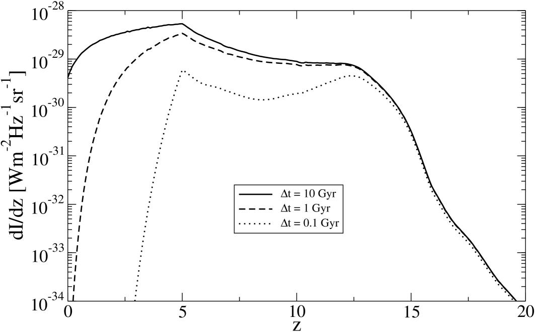
Figure 1: Intensity contribution from the dust per time-step $z$ integrated over all frequencies. This model assumes that the fraction of metals produced in stars that end up as dust is $f_{d}=0.3$. The mean dust lifetime is a largly unknown parameter, and therefore three different values are explored, $\Delta t=0.1$, 1 and 10 Gyr.

In our present model, we put the spatial distribution of the dust intensity to

$$\frac{dI}{dz}(\@vec{r},z)=\frac{dI(z)}{dz}\cdot\frac{\rho_{DM}(\@vec{r},z)}{\langle\rho_{DM}\rangle(z)},$$ (2)

where $dI(z)/dz$ is the dust intensity at redshift $z$ as measured at $z=0$ and $\langle\rho_{DM}\rangle(z)$ is the mean DM-density at redshift $z$. The MoMaF method (see Sect. 2) is then used to project the emitted intensity from the dust on a $45^{\prime}\times 45^{\prime}$ patch along the line of sight. The contribution from each simulated box is added, and the integrated dust intensity is calculated.

For $z>2.3$, the time-steps are smaller than the size of the box and each box overlaps with the next box along the line of sight. However, for $z<2.3$ the time-steps were simulated too far apart and when we pile the boxes, there will be a small part of the line of sight that will not be covered. Fortunately, this is of little consequence since the dust intensity is low at this time, and the gap is small. Each box ($45^{\prime}\times 45^{\prime}$) is divided into a grid according to the resolution that we wish to test. For Planck this means a grid that is 18$\times$18 pixels², for SCUBA 45$\times$45 pixels².

To check the normalization of the resulting intensity image, we have calculated its $\sum dI_{x,y}/N_{pix}^{2}$, where $dI_{x,y}$ is the observed intensity on pixel $(x,y)$ and $N_{pix}^{2}$ is the number of pixels², and found it to be equal to $\int dI(z)dz$ to within a few per cent.

4 Results and discussion

As described above, the MoMaF technique produces an image of the line of sight. This image represents the patch of the sky covered by the box, 150 co-moving Mpc², which translates to $\sim 45$ arcmin² at $z=14.7$. In order to avoid artifacts at the edges, the image is apodized, whereafter it is Fourier transformed into frequency space $P_{k}$. In order to convert this spectrum into spherical-harmonics correlation functions we apply the following transformation:

$$\ell=k2\pi/\theta,$$ (3)

$$C_{\ell}=\theta^{2}C_{k},$$ (4)

where $\theta$ is the size in radians of the analyzed box. These $C_{\ell}$ are then calculated at a frequency $\nu=353$ GHz, which is one of the nine Planck frequency channels. As found in Elfgren & Désert (2004), the intensity is proportional to the frequency squared, which means that the power spectrum from the dust at a frequency $\nu$ is

$$C_{\ell}(\nu)=C_{\ell}(353\textrm{ GHz})\cdot\left(\frac{\nu}{353\textrm{ GHz}}\right)^{4},$$ (5)

where $C_{\ell}$ is given in terms of $\mu$K${}^{2}_{\textrm{CMB}}$. In order to estimate an average power spectrum, 400 such images were generated and the $C_{\ell}$ were averaged over these. For comparison, we also tried to paste all these images together and calculate the $C_{\ell}$ for this (180$\times$180 pixels²) image. The result was similar to the average $C_{\ell}$. To validate our results, we also calculated the variance of the images and compared them with $\sum_{\ell}\frac{2\ell+1}{4\pi}C_{\ell}$, and found them to be compatible. The resulting power spectra can be seen in Fig. 2. The lifetime of these dust particles is a largely unknown factor, and we plot three different lifetimes, 0.1, 1 and 10 Gyrs (for a more detailed discussion of dust lifetimes, see Draine 1990). Furthermore, the dust intensity is proportional to the fraction of the formed metals that actually end up as dust, which we have assumed to be $f_{d}=0.3$. This means that the dust power spectrum is

$$C_{\ell}(f_{d})=C_{\ell}(f_{d}=0.3)\cdot(f_{d}/0.3)^{2}.$$ (6)

We note that there is only a small difference between dust lifetimes of 10 Gyrs and 1 Gyr, while the one at 0.1 Gyr is lower by a factor of four. The lowest curve in the figure represents the hydrodynamical smoothing method of distributing the dust for a dust lifetime of 1 Gyr. Naturally, it is lower than the corresponding $C_{\ell}$ for the clump method, since the DM-clumps are much more grainy (especially early in history) than the smoothed DM field. The power spectra of the two methods differ by a factor of $\sim 10$ but they do not have exactly the same form.

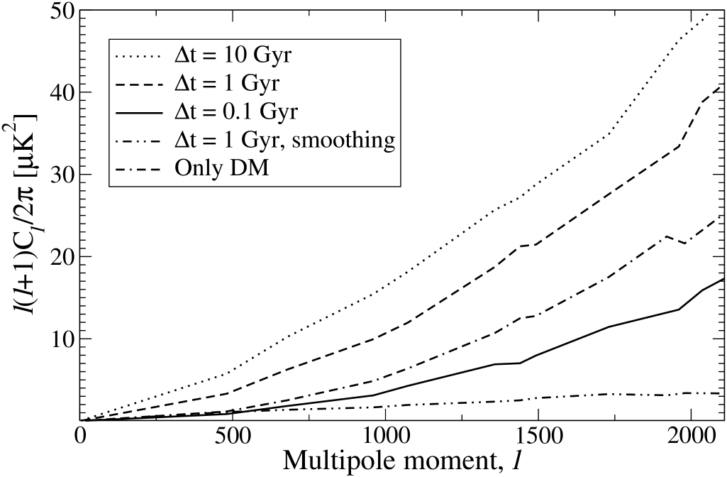
Figure 2: Dust power spectrum in CMB thermodynamic units at 353 GHz for a map $45^{\prime}\times 45^{\prime}$ and Planck resolution $5^{\prime}$ for three different lifetimes for the dust particles, 0.1, 1, and 10 Gyrs, with a solid, dashed and dotted line, respectively. The DM smoothing method for a dust lifetime of 1 Gyr is the dot-dot-dash line.

The dust frequency spectrum is distinctly different from that of other sources in the same frequency range. In Fig. 3, we compare this spectrum with that of the primoridal CMB $\Delta T$ anisotropies and that of galactic dust, $T=17$ K (Boulanger et al. 1996). In order to focus on the forms of the spectra, we normalize the three curves to one at $\nu=353$ GHz. In case of a weak early dust signal, this frequency signature could help us identify the signal by component separation spectral methods.

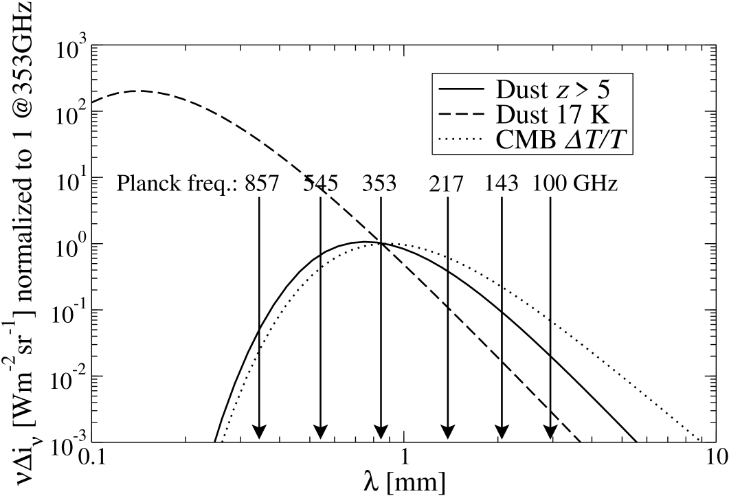
Figure 3: The form of the early dust spectrum compared to the form of galactic dust (with a temperature of 17 K) and the CMB along with indicators of the Planck HFI frequencies. The curves have been normalized to unity at 353 GHz. We see that the early dust has a special spectral signature.

4.1 Detectability with Planck

The Planck satellite, due for launch in 2007, will have an angular resolution of $30^{\prime}-5^{\prime}$ and will cover the whole sky. The Planck high frequency instrument (HFI) will measure the submillimeter sky at $\nu=$ 100, 143, 217, 353, 545, and 857 GHz. We have chosen $\nu=353$ GHz as our reference frequency. At higher frequencies, the galactic dust will become more of a problem, and at lower frequencies the CMB primary anisotropies will dominate.

In order to test the detectability of the dust with Planck, we evaluate the sensitivity,

$$\sigma=\sigma^{CMB}_{\ell}+\sigma^{instr}_{\ell}=\sqrt{\frac{2}{(2\ell+1)f_{cut}L}}\times(E_{CMB}+E_{instr})$$ (7)

(Tegmark 1997) where $f_{cut}=0.8$ is the fraction of the sky used, $L$ is the bin-size, $E_{CMB}=\ell(\ell+1)C_{\ell}^{CMB}/2\pi$ (Lambda web-site: http://lambda.gsfc.nasa.gov 1 March 2005) is the cosmic variance. The instrument error is

$$E_{instr}=C_{\ell}^{instr}\frac{\ell(\ell+1)}{2\pi}=f_{sky}\frac{4\pi s_{X}^{2}}{t_{obs}}\cdot e^{\ell^{2}\cdot\sigma_{b}^{2}}\cdot\frac{\ell(\ell+1)}{2\pi},$$ (8)

where $f_{sky}=1$ is the fraction of the sky covered, $s_{X}$ is the noise [$\mu$Ks^1/2], $t_{obs}=14\cdot 30\cdot 24\cdot 3600$ s is the observation time (14 months), and $\sigma_{b}=FWHM/2.35$ (FWHM is the full width at half maximum of the beam in radians). For Planck, the values of these parameters are given in Table 1.

Table 1: Parameters of the PLANCK HFI detector properties (The Planck collaboration 2005)

Frequency [GHz]	100	143	217	353	545	857
$FWHM$ [′]	9.5	7.1	5.0	5.0	5.0	5.0
$s_{X}$ [$\mu$Ks1/2]	32.0	21.0	32.3	99.0	990	45125

The resulting errors for a binning of $L=500$ along with the dust power spectrum is plotted in Figs. 4-5. In Fig. 4, the frequency $\nu=353$ GHz is fixed, while $\ell$ is varied. We note that $\ell\sim 1000$ seems to be a good value to search for dust. At low $\ell$, the error due to the cosmic variance dominates, whereas at high $\ell$ the instrument noise dominates.

In Fig. 5, the $\ell$ multipole binning center is fixed, and we show the electromagnetic spectrum of the primordial anisotropies and the early dust emission. The fourth point from the left in the figures corresponds to $\nu=353$ GHz and gives the best signal over noise ratio. At low $\ell$ the cosmic variance is important, at high $\ell$, the instrument noise dominates.

Early dust may therefore produce a measurable disturbance in the primordial anisotropy angular power spectrum at high multipoles (in the Silk’s damping wing). Although the primary contaminant to the CMB in the submillimeter domain is the interstellar dust emission, this new component vindicates the use of more than two frequencies to disentangle CMB anisotropies from submillimeter foregrounds.

Component separation methods for the full range of Planck frequencies should be able to disentangle the CMB anisotropies from early dust, far-infrared background fluctuations, and galactic dust emission. The Sunyaev-Zel’dovich (SZ) effect also rises in the submillimeter range but the two central frequencies of the dust, 217 and 353 GHz, can be used for its identification since the SZ-effect drops more sharply at higher wave-lengths (the SZ-effect is practically null at 217 GHz, quite different from the early dust spectrum). The spectral shape of other foregrounds can be found in Aghanim et al. (2000, Fig. 1) where we can also see that the region around $\ell\sim 2000$ is the most favorable for dust detection.

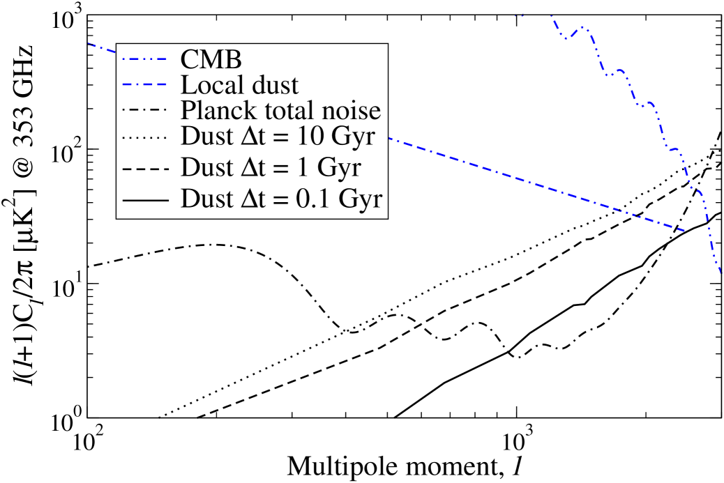
Figure 4: Comparison between dust power spectrum, the Planck error limits and local dust ($T=17$ K) at 353 GHz with binning 500. The error limits (total noise) consist of two parts; the CMB cosmic variance, which dominates for small $\ell$, and the instrument noise, which dominates for high $\ell$.

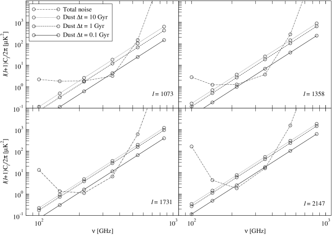
Figure 5: Comparison between dust power spectrum and Planck error limits at $\ell=1073$, 1358, 1731, and 2110 with binning 500. The error limits (total noise) consist of two parts; the CMB cosmic variance, which is constant at such $\mu$K²-levels, and the instrument noise, which has the shape of an exponential$\times\ell^{2}$.

4.2 Detectability with other instruments

There are several other instruments that might be used to detect the early dust: ALMA (Wootten 2003), BLAST (Devlin 2001), BOLOCAM (LMT) and (CSO) (Mauskopf et al. 2000), MAMBO (Greve et al. 2004), SCUBA (Borys et al. 1999), and SCUBA2 (Audley et al. 2004).

Using Eqs. 7 and 8 we have estimated the sensibilities of these detectors. The result is presented in Table 2. Since all of these instruments operate on a small patch in the sky we use $f_{sky}=f_{cut}=10\cdot FOV$, where $FOV$ is the field of view of the instrument. The integration time was set to one hour and the noise per second, $s_{X}$, was calculated as $s_{X}=NEFD/\sqrt{N_{det}}$, where $N_{det}$ is the number of detectors and $NEFD$ is the noise equivalent flux density. The error was evaluated at the multipole moment $\ell\sim 1/FWHM$ (for BOLOCAM(LMT), $\ell$ was set to 20,000), and we used a bin-size of $L=\ell$. Note that ALMA is an interferometer and thus $E_{instr}=f_{sky}\frac{4\pi s_{X}^{2}}{t_{obs}}\cdot\frac{\ell(\ell+1)}{2\pi}$ Furthermore, the SCUBA2 array needs to be renormalized such that $NEFD=NEFD\times\sqrt{N_{det}/(FOV/(\pi/4\cdot(FWHM/60)^{2}))}$. The resulting sensitivities $\sigma^{instr}_{\ell}$ can be compared with the dust signal, as plotted in Fig. 6. As can be seen, BLAST, SCUBA and MAMBO are unable to detect the dust signal. However, BOLOCAM(LMT), ALMA, SCUBA2, and BOLOCAM(CSO) have good chances of detecting the radiation from the first dust. We also note that the curves are almost parabolic. In fact, for $1,000\lesssim\ell\lesssim 100,000$ the curves can be fitted within $\sim 10\%$ as:

$$\begin{array}[]{cccccr}\ell(\ell+1)C_{\ell}^{Dust}/2\pi&\approx&2.13\times 10^{-5}\times\ell^{1.92},&\;\Delta t&=&10\textrm{ Gyr},\\ \ell(\ell+1)C_{\ell}^{Dust}/2\pi&\approx&1.37\times 10^{-5}\times\ell^{1.95},&\;\Delta t&=&1\textrm{ Gyr},\\ \ell(\ell+1)C_{\ell}^{Dust}/2\pi&\approx&4.02\times 10^{-5}\times\ell^{1.98},&\;\Delta t&=&0.1\textrm{ Gyr},\end{array}$$ (9)

in units of $\mu$K${}^{2}_{\textrm{CMB}}$. The dependency in $\ell$, which is slightly different from an uncorrelated noise $\ell^{2}$ behavior, means that large-scale correlations cannot be neglected. They mix differently at different epochs, depending on the dust lifetime parameter.

Table 2: Sensitivities, $\sigma^{instr}_{\ell}$, for different (current and future) detectors. $NEFD$ = noise equivalent flux density, $\nu$ is the operating instrument frequency, $N_{det}$ = number of detectors, $FWHM$ = full width at half max, $FOV$ = field of view in units of arcmin², $\ell=1/FWHM$, $\sigma^{instr}_{\ell}$ is the instrument sensitivity in units of mK${}_{\textrm{CMB}}^{2}$. The instrument sensitivity was calculated with Eqs. 7 & 8 using $t_{obs}=1$h, $f_{sky}=f_{cut}=10\cdot FOV$ and $L=\ell$.

Instrument	$NEFD$	$\nu$	$N_{det}$	$FWHM$	$FOV$	$\ell$	$\sigma^{instr}_{\ell}$
	$\left[\frac{\textrm{mJy}}{\sqrt{\textrm{Hz}}}\right]$	[GHz]		[$"$]	[′2]	$[10^{3}]$	[$10^{3}\mu$K2]
SCUBA	75	353	37	13.8	4.2	14	161
SCUBA2	25	353	5120	14.5	50	14	1.8
MAMBO	45	250	117	10.7	13	19	50
BLAST	239	600	43	59	85	3.5	424
BOLOCAM
(CSO)	40	280	144	31	50	6.6	0.38
(LMT)	3	280	144	6	3.1	20	1.0
ALMA	1.5	353	1	13.8/2	0.085	24	8.0

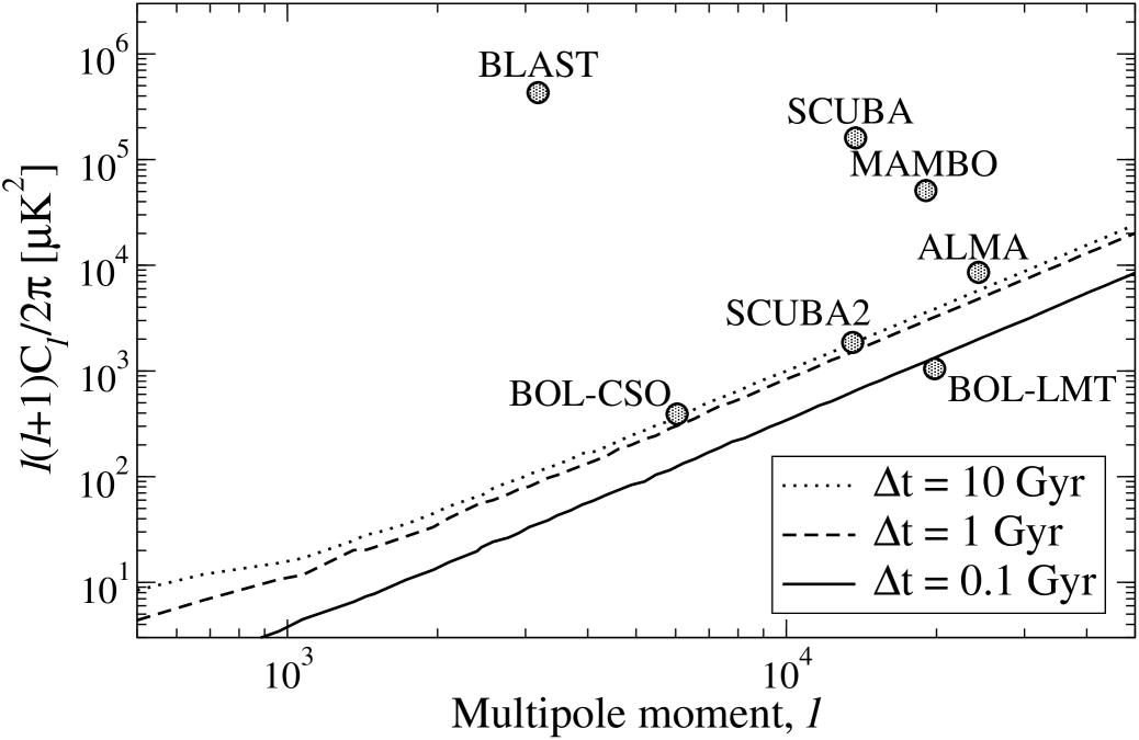
Figure 6: Dust power spectrum as a function of multipole moment, $\ell$, for different dust lifetimes. Estimated detection limits for different instruments are also included as small circles placed at $\ell\sim 1/FWHM$.

5 Conclusions

It seems that it is possible to detect the dust from the first generation of stars with the Planck satellite on small angular scales ($\ell\gtrsim 1000$). However, the detectability depends on the actual distribution of dust in the early universe, and also, to a large extent, on the dust lifetime.

The results are parametrized so that changing the frequency and the fraction of produced metals that become dust is only a matter of scaling the figures: $C_{\ell}\propto(\nu/353\textrm{ GHz})^{4}$ and $C_{\ell}\propto(f_{d}/0.3)^{2}$. The spectrum of the early dust is compared to that of the primary CMB anisotropies, as well as that of the local dust. The unique spectral signature of the early dust will help in disentangling it from the CMB and the different foregrounds (local dust and extragalactic far infrared background).

The spatial signature of the early dust is found to have $C_{\ell}\approx$ constant $\approx 10^{-5}-10^{-4}$ $\mu$K${}^{2}_{\textrm{CMB}}$ depending on the dust lifetime, $\Delta t$. Obviously, other signals that are correlated with the structures will also show a similar behavior in the power spectrum. Notably, the near infrared background from primordial galaxies could be correlated with the early dust.

The next generation of submillimeter instruments will be adequate to measure these early dust anisotropies at very small angular scales ($\ell\gtrsim 2000$). Our estimation shows that BOLOCAM, SCUBA2 and ALMA have a good prospect of finding the early dust. However, for these instruments, more detailed simulations are required in order to obtain a realistic DM and baryon distribution. A DM simulation on a smaller box, maybe $L=50h^{-1}$ for PLANCK and smaller still for ALMA, would improve the results on the relevant angular scales, $\ell\gtrsim 1000$. This also means that the particles are smaller, giving a better level of detail. Furthermore, the distribution of dust relative to the DM can also be improved and it is even possible to include some semi-analytical results from the galaxy simulations in GalICS.