Velocity-Dependent Models for Non-Abelian/Entangled String Networks
Abstract
We develop velocity-dependent models describing the evolution of string networks that involve several types of interacting strings, each with a different tension. These incorporate the formation of Y-type junctions with links stretching between colliding strings, while always ensuring energy conservation. These models can be used to describe network evolution for non-abelian strings as well as cosmic superstrings. The application to strings in which interactions are topologically constrained, demonstrates that a scaling regime is generally reached which involves a hierarchy of string densities with the lightest most abundant. We also study hybrid networks of cosmic superstrings, where energetic considerations are more important in determining interaction outcomes. We again find that networks tend towards scaling, with the three lightest network components being dominant and having comparable number densities, while the heavier string states are suppressed. A more quantitative analysis depends on the precise calculation of the string interaction matrix using the underlying string or field theory. Nevertheless, these results provide further evidence that the presence of junctions in a string network does not obstruct scaling.
I Introduction
Much of the interest in cosmic strings was lost with the realisation that they cannot be the dominant seeds for structure formation in the Universe Albrecht et al. (1997, 1999). However, their appearance in many cosmological situations forces one to consider them as subdominant contributors. Recent theoretical work in brane inflation Dvali and Tye (1999); Burgess et al. (2004); Kachru et al. (2003) and SUSY GUTs Jeannerot et al. (2003), as well as the potential for observing strings through gravitational lensing Sazhin et al. (2003, 2004); Schild et al. (2004) and the CMB Lo and Wright (2005), have contributed to a significant revival of interest in the subject (for reviews see for example Refs. Kibble (2004); Polchinski (2004); Davis and Kibble (2005); Majumdar (2005)). More recent work Battye et al. (2006); Bevis et al. (2007) suggests that CMB data allow a 10-15% contribution from cosmic strings, arguably favouring a scale-invariant spectrum plus strings over a tilted spectrum without strings.
Particularly interesting is that cosmic strings can be produced in the final stages of brane inflation Dvali and Tye (1999); Dvali et al. (2001); Burgess et al. (2001); Garcia-Bellido et al. (2002); Jones et al. (2002); Kachru et al. (2003), as D-branes and fundamental strings stretching over cosmological distances Sarangi and Tye (2002); Dvali and Vilenkin (2004); Copeland et al. (2004). These objects, often referred to as ‘cosmic superstrings’, can have different phenomenology than ordinary field theory strings. This opens up the possibility that cosmic string observations could yield information about physics at the string scale, and provides new ways of constraining various brane inflation models Babichev and Kachelriess (2005); Avgoustidis and Shellard (2005a); Brax et al. (2006); Melkumova et al. (2006). Cosmic superstrings have small tensions (in the range Sarangi and Tye (2002); Jones et al. (2003); Polchinski (2004)) and reconnect with probabilities that can be significantly less than unity Jones et al. (2003); Jackson et al. (2005). This leads to a reduced intercommutation rate, resulting in an enhancement of the predicted string number density today Jones et al. (2003); Dvali and Vilenkin (2004); Avgoustidis and Shellard (2005b). Cosmic superstring networks can consist of more than one type of string Dvali and Tye (1999); Copeland et al. (2004), which can zip together to produce trilinear vertices with links (or better, in the terminology of Ref. McGraw (1998), zippers) stretching between them. In this respect they are similar to non-abelian strings Vilenkin and Shellard (1994); Spergel and Pen (1997); McGraw (1996, 1998). In contrast to abelian string networks, which have been shown to always reach a scaling solution Kibble (1985); Bennett (1986); Albrecht and Turok (1989); Allen and Shellard (1990); Martins and Shellard (2002), non-abelian strings could in principle be frustrated Spergel and Pen (1997).
The evolution of non-abelian string networks was further studied in McGraw (1996, 1998) where some evidence for scaling behaviour was found. There have also been more recent attempts to model non-abelian strings both analytically and numerically Martins (2004); Tye et al. (2005); Copeland and Saffin (2005); Copeland et al. (2006a, b); Saffin (2005); Hindmarsh and Saffin (2006), favouring scaling (see also Ref. Avelino et al. (2006) where scaling was found for domain wall networks with junctions). In this paper we present a class of velocity-dependent models for non-abelian string evolution, developed under significantly different assumptions than those of Ref. Tye et al. (2005). In particular, rather than associating a different energy density to each type of string, while keeping a single correlation length and average velocity for all types, we associate a different correlation length and velocity to each string type and assume a Brownian network structure, in which correlation lengths also quantify string energy densities. We consider two basic categories of interactions between strings of different types, namely the coalescence along their own length (zipping) that produces a ‘zipper’, and the creation of a new segment (a ‘bridge’) of different string type as the strings pass through one another. The relative importance of these inter-related dynamical mechanisms will depend on the details of the field theory model under study, and more general interactions can be described as relative combinations of these two limiting cases, as we shall comment later. Our network evolution models are constructed in a manner close to the traditional (Kibble) approach, where the new terms corresponding to the production of bridges/zippers, are introduced through energetic considerations of string interactions within a certain volume element. We express our models in terms of the 3D energy density of strings, thus ensuring the use of well established techniques in calculating the energy loss of the long string network. We can then directly compare our results to both the usual (3D) VOS model Martins and Shellard (2002) and numerical simulations Bennett and Bouchet (1990); Allen and Shellard (1990).
Central to our models is ensuring that energy is conserved by balancing the energies corresponding to the produced and lost string lengths and/or the kinetic energies of the interacting and produced string segments. In this way we avoid the possibility of finding ‘spurious scaling’ by artificially throwing away energy from regions of intercommutation. Realistic collisions can of course be inelastic, in that some of the energy can be released in the form of radiation. This provides an additional energy loss mechanism, which facilitates the reaching of a scaling regime. In the absence of a quantitative understanding of the importance of such an energy loss mechanism, we take a conservative approach and assume energy balance at the interaction regions. We find that even in this case, where this potentially important energy loss mechanism is effectively switched off, multi-tension networks with junctions can still reach scaling.
The structure of the paper is as follows: In section II we briefly review some basic facts about cosmic string evolution both in the abelian and non-abelian case. In section III we move on to construct a class of velocity-dependent models for non-abelian string evolution. Application to strings is presented in section IV, whereas in section V we consider the case of cosmic superstrings. Our conclusions are summarised in section VI.
II Cosmic String Evolution
II.1 Abelian Strings
Most well-studied examples of cosmic strings are those arising in theories with a broken symmetry, like the Nielsen-Olesen vortex lines of the abelian-Higgs model. Understanding the interaction of strings when they intersect is crucial for modelling their cosmic evolution. For such strings, crossing has two topologically allowed outcomes: either the strings pass through one another, or they intercommute (reconnect) by exchanging partners. Which situation is actually realised is a dynamical question. This problem has been extensively studied numerically in field theory Shellard (1987); Matzner and Mccracken (1988), where it was found that the strings reconnect with probability of order unity111See Ref. Achucarro and de Putter (2006) for a recent study of possible exceptions to this rule in high-velocity regimes.. Some recent analytic results have also been presented in Ref. Hanany and Hashimoto (2005). Having quantitative understanding of string-string interactions is necessary for modelling the cosmological evolution of strings. Below we review some basic results.
II.1.1 Basics
Numerical simulations of string formation in field theory suggest that strings formed after cosmological phase transitions have, to a good approximation, the shape of random walks. This allows one to describe a string network by a characteristic length , which determines both the typical radius of curvature of strings and the average interstring distance. There is typically one string segment of length in each volume so that the energy density of the network can be defined as
| (1) |
As the network evolves, strings collide with each other or curl back on themselves creating small loops, which oscillate and radiatively decay. Via these interactions enough energy is lost from the network to ensure that the strings do not dominate the energy density of the universe222Energy loss through production of particles could also play a significant role Vincent et al. (1997); Moore et al. (2002b). . An approximate energy loss rate equation can be written Kibble (1985)
| (2) |
where the first term is due to Hubble expansion ( being the scalefactor of the universe) and the second term models the energy lost through string interactions and the formation of loops. Such interacting networks are known to evolve towards a so-called ‘scaling’ regime in which the characteristic length stays constant relative to the the horizon Kibble (1985). This can be seen by setting and substituting (1) into (2) to obtain
| (3) |
The expansion exponent is related to the scalefactor by and is equal to and in the radiation and matter eras respectively. Equation (3) has indeed a scaling solution
| (4) |
demonstrating that the characteristic length asymptotically reaches a constant value with respect to the horizon . If one starts with a high density of strings, intercommuting will produce loops reducing the energy of the network, whereas if the initial density is low then there will not be enough intercommuting and will decrease. Given enough time, the two competing effects of stretching and fragmentation will always reach a steady-state and the scaling regime will be approached.
The above discussion captures the key physical processes involved in string evolution, but for a more quantitative study one needs models of higher sophistication. String evolution has been extensively studied numerically through Nambu-Goto simulations Albrecht and Turok (1989); Bennett and Bouchet (1990); Allen and Shellard (1990), verifying the above picture, but a number of analytic models have also been developed. These include a velocity-dependent one-scale (VOS) model Martins and Shellard (1996a, b, 2002), a ‘kink-counting’ model Allen and Caldwell (1990); Austin (1993), a functional approach Embacher (1992), a ‘three-scale’ model Austin et al. (1993) and a ‘wiggly’ model Martins (1997). In the following we will consider the VOS model, as it is the simplest of these and has been shown to be in very good agreement with numerical simulations Moore et al. (2002a).
II.1.2 The VOS model
The velocity-dependent one-scale (VOS) model is a simple analytic model, depending on one free parameter only, which agrees quantitatively with Nambu-Goto string evolution simulations. From the theoretical point of view it is well-motivated and can be obtained directly from the Nambu-Goto action, by performing a statistical averaging procedure on the string equations of motion and energy momentum tensor along the network Martins and Shellard (1996a). In particular, from the energy momentum tensor one can obtain an evolution equation for the string energy density , whereas the Nambu equations of motion yield a ‘macroscopic’ equation for the evolution of the typical rms velocity of string segments.
The resulting equations are:
| (5) |
| (6) |
The second term in equation (5) is a phenomenological term which takes into account the energy losses through creation of loops. This depends on the loop production parameter , related to the integral of an appropriate loop production function over all relevant loop sizes Vilenkin and Shellard (1994). In equation (6), is the average radius of curvature of strings in the network and the so-called momentum parameter (see later discussion) introduced in Ref. Martins and Shellard (1996a). For a Brownian network, and within the VOS assumptions, the average radius of curvature can be taken equal to the correlation length .
This is of the same form as (3) but has an extra correction term accounting for redshifting of velocities due to cosmological expansion. It also includes the parameter , the value of which can be extracted from numerical simulations and it is of order unity Vilenkin and Shellard (1994); Martins and Shellard (1996b). Possibly reduced intercommuting probabilities relevant to cosmic superstrings, or non-intercommuting for high velocities in type II strings Achucarro and de Putter (2006), correspond to a smaller effective value of .
The system (6-7) has the scaling solution
| (8) |
in terms of the expansion exponent , the loop production parameter , and the momentum parameter which is a measure of the smoothness of the strings. An accurate ansatz for the momentum parameter has been proposed in Martins and Shellard (2002)
| (9) |
which incorporates the ‘Virial’ condition , observed in Nambu-Goto simulations Vilenkin and Shellard (1994).
With this ansatz the VOS model depends on one parameter only, , which, as mentioned above, can readily be extracted by comparison to numerical simulations. Remarkably, by adjusting this parameter once only, one can closely model high resolution Nambu-Goto simulations throughout cosmic history.
II.2 Non-Abelian Strings
Consider a situation where a gauge symmetry group is spontaneously broken to a subgroup . This process can give rise to topological defects classified by the homotopy groups of the vacuum manifold . In particular, string defects can occur if the vacuum manifold is not simply connected that is , where is the fundamental group and the identity. In the example of strings the symmetry breaking is so , the group of integers, corresponding to the integer winding number of strings. For a connected and simply connected gauge group, the fundamental theorem implies , where is the set of disconnected components of . Thus, for a simply connected , strings can occur if is disconnected.
The flux of a string is given by a path-ordered exponential of the gauge field Alford et al. (1992)
| (10) |
where is a closed, oriented path, which encloses the string without passing from the string core and without enclosing any other strings. The requirement that the Higgs field which drives the symmetry breaking is invariant under parallel transport along such a closed path forces the flux to be an element of the unbroken group . If is non-abelian then the above definition is not gauge invariant: under a gauge transformation by the flux changes to . However, two paths which start and end at the same point and which can be continuously deformed to each other necessarily have the same flux.
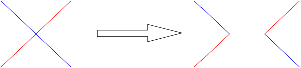
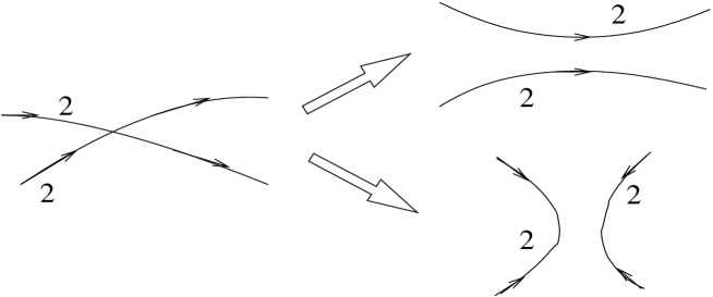
The non-abelian structure of gives rise to a certain degree of ambiguity in defining the flux of a particular string. Consider a string A which is entangled to another string B as in Fig. 1.

One can calculate the flux on one side of by considering the path , and the flux on the other side by considering path . Since strings A and B are entangled, path cannot be deformed to without encountering string B. Therefore, they correspond to different elements of the fundamental group and the fluxes and are generally different. In fact they are related by conjugation with the flux (of string B, corresponding to path ) that is
| (11) |
which gives in the abelian case. This is not merely a mathematical curiosity, but a physical effect that can be interpreted in terms of a long-range interaction between non-commuting strings, the so called ‘holonomy interaction’ Bucher (1991); Wilczek and Wu (1990); Alford et al. (1992). Thus, the flux of a particular string is not associated to a unique element but can be described by several distinct conjugate elements of . It follows that strings with fluxes in the same conjugacy class must have the same tension.
Non-commutativity of changes the nature of string interactions, thus giving rise to an interesting property of non-abelian strings: the ability to form entangled networks. Indeed, two strings carrying non-commuting fluxes can neither pass through each other nor reconnect, as both possibilities would violate flux conservation Toulouse (1976); Mermin (1979). The collision of two such strings leads to the formation of a new string segment stretching between the two, which carries flux given by the commutator of the initial fluxes. A related process is that of branching, that is the splitting of a string with flux to two strings with fluxes and . This is not however special to having a non-abelian unbroken group ; it can also occur for strings arising through the process , with McGraw (1996); Aryal et al. (1986); Vachaspati and Vilenkin (1987). Also, for type I strings, colliding segments can zip for small enough crossing angle and velocity of approach Bettencourt and Kibble (1994).
The evolution of entangled and/or branched networks is not as well understood as that of ordinary string networks. A certain class of non-abelian strings have been studied numerically in Ref. Spergel and Pen (1997), where the possibility of a ‘frustrated’ network (one that does not exhibit the scaling property and eventually dominates the energy density of the universe) was identified. Simulations of strings were presented in Refs. McGraw (1996, 1998), where strong evidence for scaling behaviour was found. Interest in the subject has recently revived in the context of ‘cosmic superstring’ networks, which also have the branching property. Recent attempts to model such networks both analytically and numerically can be found in Refs. Martins (2004); Tye et al. (2005); Copeland and Saffin (2005); Saffin (2005); Hindmarsh and Saffin (2006). In particular Ref. Martins (2004) suggests a way to generalise the VOS model to take into account the formation of links (or ‘bridges’) in an entangled/branched network. Ref. Tye et al. (2005) proposes a further generalisation in order to model networks composed by different types of strings, each with different tension. Finally, Refs. Copeland and Saffin (2005); Saffin (2005); Hindmarsh and Saffin (2006) take a field theory approach to cosmic superstring models.
The aim of this paper is to develop an analytic model for the evolution of multi-string, entangled/branched networks in the spirit of Refs. Martins (2004); Tye et al. (2005). Our work closely follows the traditional Kibble approach to modelling string-string interactions in terms of energetic considerations in a correlation length volume. We start developing our models in the next section.
III Non-Abelian VOS models
We wish to study a network of cosmic strings consisting of several different types of string, possibly with different tensions and non-commuting fluxes. The two mechanisms governing the evolution of the network are the cosmological expansion (with its associated velocity redshift effects) and the string-string interactions. For U(1) strings both effects are well-described by the VOS model, but to allow for the new possibilities arising in a multi-string network (section II.2) this model needs to be accordingly modified. As in Ref. Tye et al. (2005) we aim to have a set of VOS equations for each type of string, with extra terms added in order to describe the interactions between different string types which transfer energy from one type to another.
String interactions are modelled as follows: when two strings of the
same type collide there are two topologically allowed outcomes;
either they intercommute or pass through one another. This will be
described by the usual VOS parameter (see Eq. (5)),
parametrising the energy lost through self-intersection of strings and
the subsequent production of loops of the same type. However, if the
collision involves different types of strings (with non-commuting
fluxes) then both the above possibilities violate flux conservation.
The collision instead leads to the production of a new string segment,
joining the two strings 333Here we neglect the more complex
mechanism by which loops consisting of several types of string are
lost to the network.. As already mentioned we choose to describe
the formation of the new segment via two inter-related limiting
mechanisms:
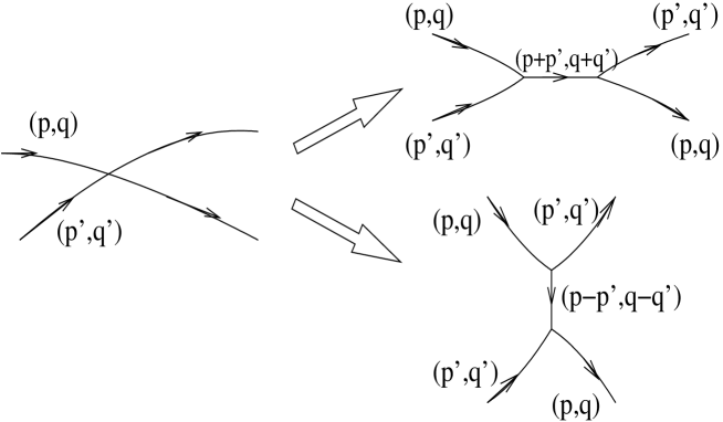
(i) The strings pass through one another and in doing so
they become linked by a new string segment of a third type
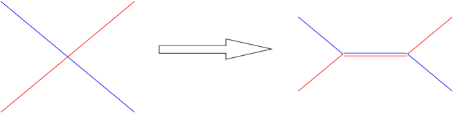
(Fig. 2). This is the so-called ‘bridge’
configuration in the terminology of Ref. McGraw (1998).
In this asymptotic limit the energy to make the new link
is acquired from the kinetic energy of the original pair.
(ii) The strings coalesce along part of their own length,
in the so-called ‘zipper’ configuration of Fig. 3.
In this limit there must be significant energy gain from the
realignment and coalescence of the two original strings, which
lose physical length to create the new segment.
A general model will involve some combination of these two limiting mechanisms. Their relative importance is both a dynamical and kinematic question depending on the string tensions, velocities and angles between the colliding strings, as well as topological considerations. Model-dependent averages, such as those considered in Refs. Copeland et al. (2006a, b), may be used to determine their relative quantitative importance. We will first consider the impact of each of these possibilities separately in sections III.1.2 and III.1.3. Then we will present the general case with both mechanisms incorporated to describe more general string interactions.
III.1 Toy Models
Consider a simple example where we begin with a network of Brownian strings of types and , with tensions , and correlation lengths , respectively. We can think of this system as two separate networks, each characterised by its own correlation length, which are allowed to interact with each other. Interactions between strings of the same type are as in the case, but when strings of type and collide they produce a new segment of type with tension . We assume that the energy density of segments of type 3 can be described by a correlation length , as for a Brownian network. We can then define the energy density and write an evolution equation
| (12) |
The first two terms are as in Eq. (5) and describe the effects of cosmological expansion and loop production through self-intersection of strings of type . The third term models the production of new segments of type string from interactions between strings of types and .
To write down a formula for we consider a correlation-length-sized segment of type string interacting with the type network and take, without loss of generality, . On average there is one type segment of length in each correlation volume , so that, if is the velocity of the type segment relative to the (type ) network, then the probability that the segment meets a string of type in time is:
| (13) |
Such a collision results in the production of a new type segment. In analogy to the case of loop production, we will assume that the length distribution of the produced links is peaked at a value . Integrating over this distribution function introduces an efficiency parameter , the analogue of parameter for the case of loop production. Considering that on average there are strings of type in each cube of volume we can write
| (14) |
Note that this expression is symmetric in as expected.
With equation (14) modelling the production of links due to interactions of strings of different type, and with the assumption that the produced links form a Brownian network, we can go on to construct simple VOS models of non-abelian string evolution. We will first consider toy models of networks consisting of three types of string only, which interact in a simple manner, and in the next sections we will progressively build more complex models. Before presenting the models we briefly discuss the important issue of energy conservation.
III.1.1 Energy Conservation Issues
When considering macroscopic string evolution equations, it is important to make sure that energy is conserved by the interactions. In the 3D VOS model, the loop production term damps energy from the long string network, but this energy is simply transferred to the network of cosmic loops. However, for processes where two colliding long string segments produce a (long) segment of third type, it is important that the energy differences balance exactly, so that no net energy is produced or lost. If this condition is not met, one is in danger of unphysically throwing energy away, which may lead to a ‘spurious’ scaling regime. Of course, string collisions may well be inelastic, and it seems plausible that some energy can, indeed, be lost through particle production Moore et al. (2002b); Vincent et al. (1997) or gravitational radiation. However, it is at present not clear what proportion of the relevant energies can indeed be damped away from the network through, say, massive radiation. In the case of Abelian-Higgs networks, there is evidence that massive radiation is subdominant compared to loop production and gravitational radiation decay mechanisms Moore et al. (2002b).
In the absence of a quantitative understanding of particle production in the present context, it seems dangerous to assume that the energy difference associated to the zipping, say, process is all damped away through this decay channel. A more conservative approach would be to impose energy conservation during string intercommutations (in other words to switch off particle production), and see whether the resulting networks can still reach a scaling regime. That is the approach we will follow in this paper. As we will see, for interactions of the bridge type, this energy balance can be accomplished by taking into account the slowing down of the original strings due to the tension of the bridge between them, or, in the zipper case, by giving kinetic energy to the produced zipper through terms in the corresponding velocity evolution equations. We now examine each of these situations separately.
III.1.2 Model with Bridges
Now consider the case where strings of type and produce type segments through interactions of the ‘bridge’ type (Fig. 2). As the strings pass through one another, a new segment of type is produced, while the initial length of each of the original strings is preserved (Note that by ‘length’ we mean physical, not invariant, length). The tension of the formed link slows down the original strings, and in doing so its length increases. If is the average value of the lengths of the links at the end of all interactions which occurred at times around , then the evolution of the energy density of the type network is given by Eqs. (12) and (14). However, since the length of type and strings is not affected by the production of bridges, the corresponding evolution equations for networks and will be of the form of Eq. (5). We will therefore have for the energy densities:
| (15) |
| (16) |
Equations (15)-(16) seem to violate energy conservation since for (flat space) and (no loop production), the first two equations become but has a positive term, appearing to create energy from nothing. This energy is actually coming from the kinetic energies of the colliding strings (which have been slowed down due to the tension of the bridge stretching between them) and needs to be taken into account in the velocity equations. To do this, we express the string density in terms of the proper correlation length , taking into account relativistic length contraction of a moving string in a box of size :
| (17) |
where is the Lorentz factor associated with the motion of the string. We can then convert changes in string energy density to string accelerations via the equation
| (18) |
We have one such term for each string of type and and we require that they balance the energy gain due to the production of bridges, that is
| (19) |
Since the strings can have different tensions, the weighting depends on the relative string tensions 444One could also consider dependence on correlation lengths and/or string velocities., so we introduce two weighting factors , such that and require
| (20) |
| (21) |
Using Eqs. (18) and (14) we find
| (22) |
which are the new terms we seek. The velocity evolution equations for our model are therefore
| (23) |
| (24) |
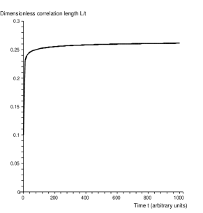
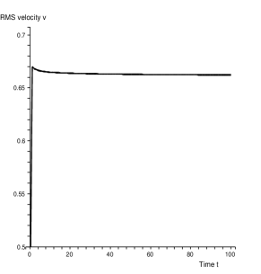
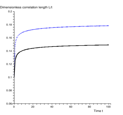
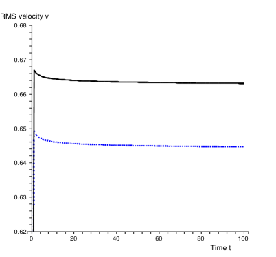
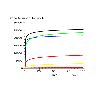
This picture is not complete, as we have not specified what happens when a string of type collides with strings of type or . For this toy model we will simply assume that the strings simply pass through one another in such an encounter, but more complicated models of this type will be considered in section IV. Our aim here is to describe how such multi-string models may be constructed and to demonstrate that the presence of different string types in the network, interacting with each other through terms like (14), does not necessarily obstruct string scaling. Indeed, taking all loop production parameters , and equal to the canonical value (coming from Nambu-Goto simulation of a single string network Martins and Shellard (1996b)) and solving Eqs. (15)-(16), (23)-(24) numerically, we find scaling behaviour for all three string types. This is illustrated in Fig. 4 for , . For the weighting factors we have taken and , since the light string’s motion is affected more due to its smaller inertia. We see that in this model, type strings (shown in a blue dotted line) have smaller and therefore become more abundant than types and . This is simply a consequence of the fact that we have not allowed the breaking of type strings into types and : type strings are continuously produced by interactions between type and strings, while there is no such mechanism to produce string types or . Also note the important differentiation between string types 1 and 2. This is because of the velocity dependence (see Eq. (23)), since type 1 strings with less inertia lose more kinetic energy in an interaction. Lower velocities imply lower interaction rates for loop production which enhances the overall density of the light string.
From the point of view of string density evolution, a scaling solution is generically reached, as can be seen directly from the corresponding equation:
| (25) |
Each term in the right hand side of (25) has a different dependence on . Further, the loop production term tends to increase , but as this happens this term weakens. Similarly, the term corresponding to the production of bridges tends to reduce and in doing so it also weakens. Thus, there is always a value of for which the right hand side of (25) is zero (scaling) and the dynamics is such that the system is driven towards that value. However, if we allow interactions between type 3 and type 1 or 2 strings by including bridge production terms in equations (15), then decreasing of , in the bridge production term of equation (25) could in principle lead to a frustrated network. It is therefore important to consider more complicated situations separately, which we will do in section IV.
III.1.3 Model with Zippers
Now consider the case where collisions between strings of type and produce type segments through interactions of the ‘zipper’ type (Fig. 3). In this case the original strings coalesce along their own length, so there will be extra terms in the corresponding energy density equations, describing the energy loss associated to the length of the colliding string which was converted to type . The energy density evolution equations thus become:
| (26) |
| (27) |
In general so there will be an energy density of
| (28) |
left from the interaction. We impose energy conservation by demanding that this energy excess is given as kinetic energy to the produced zippers, that is we require
| (29) |
This corresponds to the introduction of a new source term in the velocity equation of type strings. The velocity evolution equations for this model are then
| (30) |
| (31) |
As explained above (section III.1.1), imposing energy conservation at zipping is a conservative approach, which corresponds to switching off the possibility of damping energy through particle production or gravitational radiation. In this way we avoid the possibility of artificially throwing away too much energy, which could lead to an unphysical scaling regime. The main purpose of this paper is to demonstrate that loop production alone can still provide an efficient damping mechanism in the presence of links, so that we will assume energy conservation throughout the paper. When using phenomenological models of the type we present here to fit simulations, one can easily relax this assumption by introducing a tunable unbalance through reduction of the coefficient in equation (31).
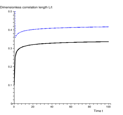
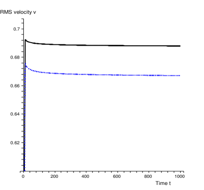
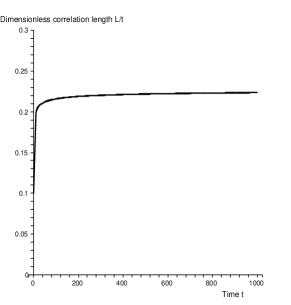
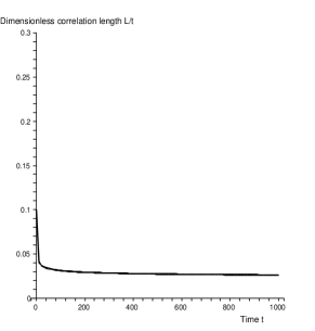
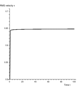
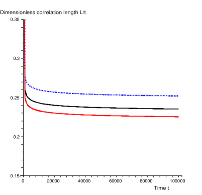
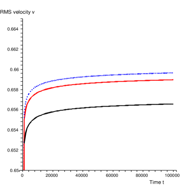
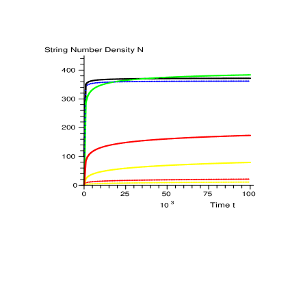
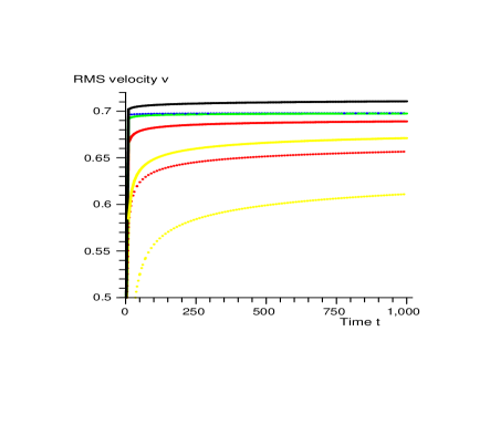
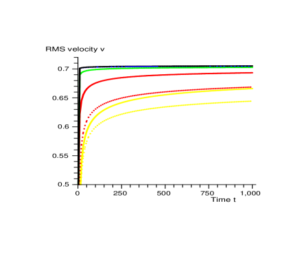
Solving Eqs. (26)-(27), (30)-(31) numerically with we find scaling for all string types (Fig. 5), where, as before, the heaviest type strings are more highly populated. Again, this is because we have not included the possibility of ‘unzipping’ of type strings through their collisions with type or : string length is continuously lost from type and strings into forming type zippers, but the type network only loses length through loop production. Allowing for the possibility that strings of type collide with type (resp. type ) producing type (resp. type ) segments one also finds scaling solutions were the most massive type 3 strings are less heavily populated (Fig. 6). We see therefore in this toy model that all string interactions have to be taken carefully into account, in order to obtain the correct scaling. We will construct more complicated models of this type in section V.
III.2 General Case
Arbitrarily complex models of multi-string networks can be built in a similar way by replicating the VOS equations (5),(6) and adding extra terms of the type discussed above. The result is a tower of ODE’s of the form
| (32) |
| (33) |
where denotes the efficiency parameter for the process in which strings of type and interact to produce a type segment, is the average relative velocity between strings of type and , whereas is the average length of links of type , produced by interactions between strings of types and around time . The first sum in Eq. (32) represents the energy lost from network due to the length of type strings that coalesced with other types to produce zippers. Note that no length from the colliding strings is lost when a bridge is produced (see section III.1.2) so the sum is constrained only on interactions of the zipper type. On the other hand, the second sum models the energy gain of network due to the production of both bridges and zippers of type . Similarly, the first sum in Eq. (33) describes the slowing down of strings of type due to their attachment to a newly formed bridge when they interact under the bridge configuration, while the second sum corresponds to the kinetic energy that must be given to zippers of type to ensure energy conservation. More general string interactions can be modelled as combinations of the bridge and zipper types, and the relevant weighting can be encoded in the coefficients . Also, as mentioned above, one can relax the assumption of energy conservation at string interactions, to include the possible effect of energy release through particle production Vincent et al. (1997); Moore et al. (2002b), by modifying some of these coefficients so that string mass-lengths and kinetic energies are not precisely balanced.
Working as in sections II.1.1, II.1.2 we introduce the functions and rewrite Eqs. (32)-(33) in the following form
| (34) |
| (35) |
Eqs. (34)-(35) can be applied to any given model of multi-string network evolution, specific examples of which will be considered in sections IV and V.
Before moving to these applications, we comment on the size of segments produced in non-abelian interactions which is, in principle, another variable. One expects this to be a function of the correlation lengths of the colliding strings as well as the string velocities. In Ref. Martins (2004), was expressed in terms of a constant ‘zipping velocity’ , as . In Ref. Tye et al. (2005) on the other hand, all string types have the same correlation length and all interactions are of the zipper type, so one can safely assume . Here, each string species has its own correlation length so we cannot adopt this approach. Instead we will consider bridge-type and zipper-type interactions separately and propose physically motivated ansatze.
For bridge interactions, the original strings do not lose length but are slowed down due to the tension of the bridge formed between them. Therefore, given the tensions of all strings involved and the velocities and correlation lengths of the colliding segments, one can impose local energy and momentum conservation to find the length of the produced bridge. For comparable string tensions and correlation lengths, the following approximate formula holds for the length of the produced bridge:
| (36) |
This is the formula we used in our bridge toy model, and we will also use it in section IV, where we will study the evolution of strings with similar tensions, through a bridge-type model. Note that this is the maximum possible length that can be created because all the kinetic energy of the parent strings is lost in stretching the bridge to a length . By integrating over different string orientations, it is clear that the average bridge length will be significantly less than in equation (36), which corresponds to the parameter being significantly smaller than unity .
In the zipper case both of the interacting strings lose the same amount of length (which also equals the length of the produced zipper) and, since string direction changes after correlation length distances on the string, this cannot be larger than the smallest of the two correlation lengths. We could choose but this would not be easy to implement in the equations. Instead, we will take
| (37) |
a simple expression which returns a value smaller than, but not far off, the smallest of the two correlation lengths. This is a good approximation to the smallest correlation length if , differ by an order of magnitude or more, and it returns half the correlation length for . This is not however a problem, as the corresponding term in the evolution equations comes with a coefficient , a free parameter of the model in which we can absorb this normalisation. The important issue is to make sure that has the correct scaling. We will also use this ansatz when modelling -strings with zipping interactions in section V.
For more general interactions, interpolating between the two, the ansatz for will depend on the specific model under study. Finally, for the collision velocity between strings of type and we will take the magnitude of the relative velocity vector , averaged over directions, namely .
IV Application to strings
Consider a situation in which a continuous, simply connected group is spontaneously broken to . Let (where ) parametrise a closed curve in physical space and denote the vacuum at position by . Then there is a group element which maps the vacuum at to that at , that is . Now consider the unbroken group at with elements . The curve under consideration will encircle a string if . One would like to associate a different type of string to each non-trivial group element of the unbroken group. However, the group structure of imposes relations among various elements, which, under certain circumstances, allow one to identify strings corresponding to different group elements.
To see this, consider the cyclic group , which only has one generator and elements . Acting on with the generator gives back the identity, that is . By rewriting this as we see that strings corresponding to elements and have opposite fluxes. In some cases, depending on the details of the symmetry breaking process, such strings and antistrings have been found to be connected by monopoles Hindmarsh and Kibble (1985); Aryal and Everett (1987), and the evolution of such monopole-string networks has been discussed in Ref. Vachaspati and Vilenkin (1987). However, if the symmetry breaking process does not give rise to monopoles, each string and its corresponding antistring are topologically equivalent Aryal and Everett (1987); Aryal et al. (1986). In particular, groups and give rise to one type of string only, while the lowest order cyclic group which admits more than one distinct strings is .
Note however that branching can occur in networks too Aryal et al. (1986), even when there is effectively only one type of string (see also Ref. Bettencourt and Kibble (1994)). To see this, consider a volume element in physical space and assume that an string enters from one side. Charge conservation requires that the same amount of flux must leave the volume and this can be satisfied, for example, if an string also exits the volume from the other side, corresponding to the situation of a single string transversing the volume element 555Since for we have , this can also be seen as an string entering the volume and joining with the incoming string.. However, since , flux conservation is also satisfied if two strings enter from the other side, corresponding to three incoming strings joining at a vertex and forming a Y-type junction. But so this can also be seen as an string branching into two (outgoing) strings, two strings joining to an , or three strings emerging from a 3-string vertex. From the point of view of string evolution Vachaspati and Vilenkin (1987), and strings can be identified and the above configurations are equivalent.
IV.1 Modelling networks
In order to apply our string evolution model to a given string network, we need to study the topologically allowed outcomes from interactions between different types of string. This will allow us to set some of the of equations (34)-(35), namely those corresponding to topologically forbidden interactions, to zero. Consider for example the case of , which has elements . There are three types of string corresponding to , and . Since two strings of type 1 can join to a single type 2 string. Thus, two intersecting type 1 strings can either exchange partners or form a type 2 string segment (bridge) between them (Fig. 2). Similarly, type 1 and type 2 strings can join to a single type 3 string, as (Fig. 3). Also, since , two type 2 strings can end on a vertex and so, depending on the details of the relevant symmetry breaking, either they are linked by a massive monopole or kink Hindmarsh and Kibble (1985), or they are self-conjugate Aryal and Everett (1987). In either case, the crossing of two type 2 strings can have two outcomes, as shown in Fig. 7. The presence of a massive monopole at the vertex where the strings meet does not directly affect macroscopic string evolution. Since monopole creation requires energy, such a configuration can result from high energy collisions only. This can be taken into account in our models by choosing an appropriately small efficiency parameter for such energetically disfavoured processes. As with type 1 strings, two type 3 segments can join to a single type 2, because . Finally, so a type 1 and a type 3 string can also end at a vertex. Then strings of types 1 and 3 can be seen as the same string, with opposite orientation.
In the above example of strings we see that, although two colliding type 1 strings can form a bridge of type 2 string, intersecting type 2 strings can only exchange partners. Thus we have , in (34)-(35). Also, the intersection between strings of type 1 and 2 can only lead to the formation of a type 1 bridge () but not type 2 (). The parameters and can be grouped in a matrix
| (38) |
A discussion of the topologically allowed outcomes of string collisions and the corresponding parameter matrices for the cases of , and can be found in the appendix.
For non-abelian string networks, string-string interactions are governed predominantly by topological, rather than energetic, considerations, except in extreme parameter regimes (e.g. strongly Type I strings). A link is produced between two colliding segments because this is the configuration which conserves charge, not because it minimises energy. Energy gains or losses associated to the colliding strings converting their length to the new string type are only marginal in general. Thus, one expects that such interactions can be approximated by those of the bridge type, in which the interacting strings are not losing length but the link forms and slows them down due its tension. We will now apply a bridge-type model to the above cases of strings.
IV.1.1 strings

The simplest case allowing the formation of Y-type junctions is , where there is only one type of string and the collision between two string segments can either lead to reconnection or to the production of a bridge. The corresponding VOS model describing the evolution of such a network is given by the equations (see Eqs. (34)-(35))
| (39) |
| (40) |
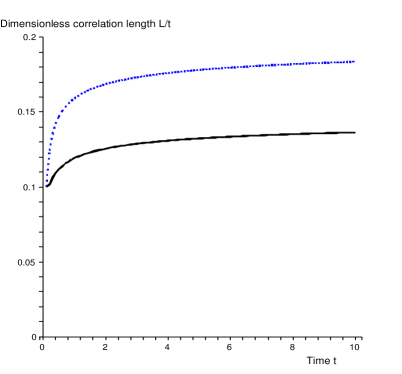
where is the average relative velocity of strings and all other parameters/variables are as described in the text. Solving this system with we find (Fig. 8) scaling solutions for . The larger is, the more entangled the network becomes and the scaling solution moves from its ‘abelian’ value to one with higher string density. For the network becomes so dense that the bridge production term dominates, driving the system to an even denser state and thus spoiling scaling. In view of the discussion of last paragraph of III.1.2 this happens in the case of because both the interacting strings and the produced bridge are of the same type, so the dependence of the bridge production term on changes from to . Then if this term gets to dominate, the string density increases ( decreases) and the term becomes even stronger, so that scaling cannot be achieved. However, since intercommuting is energetically favourable compared to bridge production, one expects . Then the formation of Y-type junctions increases the string density (Fig. 8) but does not spoil the scaling property of the network.
IV.1.2 strings
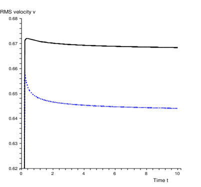
For there are two types of string, say type 1 and type 2, and the corresponding parameter matrix is given by (38). A network can therefore be described by two copies of equations (34)-(35) with non-zero parameters , , and (and with all zipper terms set to zero). Again scaling solutions can be found when the bridge production terms do not dominate. For type 1 strings, since reconnection is energetically favourable compared to bridge production, we will assume . For collisions between type 1 and 2 strings, however, reconnection is not possible and the production of a type 1 bridge is the only option, so that can be large. One then finds scaling as long as does not exceed a critical value, which depends on the chosen . For example choosing , (Fig. 9) we find scaling, for both string types, for .
IV.1.3 strings
networks also consist of two types of string but with different interaction rules (see appendix). The parameter matrix is given by (48) and the relevant VOS model arises by the appropriate adaptation of two copies of equations (34)-(35). Again, both string types achieve scaling when are not larger than (Fig. 10).
IV.1.4 strings
In the case of there are three distinct types of strings (see appendix) with parameter matrix (49). The system is modelled by three copies of (34)-(35). All three string types reach scaling for small enough ’s (Fig. 11).
IV.1.5 strings
Here there are also three string types with parameter matrix (50). The relevant scaling solutions are shown in Fig. 12.
V The case of cosmic superstrings
In this section we apply our model to cosmic superstrings, typically produced at the end of brane inflation Dvali and Tye (1999); Dvali et al. (2001); Burgess et al. (2001); Garcia-Bellido et al. (2002); Kachru et al. (2003). In this picture, a brane-antibrane pair are moving towards each other under their attractive interaction, and in doing so they give rise to an inflationary phase. Inflation ends when the branes collide and annihilate, leaving behind a network of D- and F-strings Burgess et al. (2001); Sarangi and Tye (2002); Jones et al. (2003); Dvali and Vilenkin (2004); Jackson et al. (2005). String interactions can lead to the formation of bound states between F-strings and D-strings, referred to as -strings, where are coprime 666If are not relatively prime, the string is just a collection of lighter coprime strings.. This situation corresponds more closely to interactions of the zipper type, rather than bridge production, as the strings coalesce along their own length in forming a bound state. Also, unlike strings, where different string types could have the same tension, here each type of string has different tension. F-strings, being perturbative objects have tensions proportional to the square root of the string coupling, namely
| (41) |
while D-strings are non-perturbative and have
| (42) |
In flat space777For the corresponding formula in warped space see Ref. Firouzjahi et al. (2006). String evolution in this context has been studied in Leblond and Wyman (2007); Avgoustidis (2008). the tension of strings is given by
| (43) |
V.1 Modelling superstring networks
To model cosmic superstring networks we consider two types of elementary string, type 1 with tension (corresponding to the F-string) and type 2, tension (the D-string). When two elementary strings of the same type collide, they may pass through one another or reconnect by exchange of partners. However, a type 1 and a type 2 string can bind together to form a string segment. In general, when a and a string collide they can bind in two ways, depending on the angle of collision Tye et al. (2005); Jackson et al. (2005); Copeland et al. (2004), forming either a or a segment (Fig. 13), where without loss of generality we have taken .
Given that binding has taken place, the probability that the additive/subtractive process has occurred is given by Tye et al. (2005)
| (44) |
where we have assumed that the RR scalar is zero. Assuming that the zipper type interaction is a good approximation to this binding, we can model such a network by equations (34)-(35) with zero bridge terms and
| (45) |
with ’s in the range found in Ref. Jackson et al. (2005).
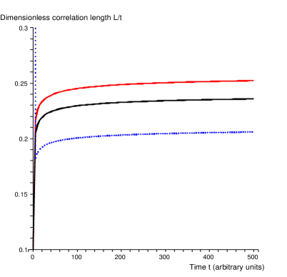
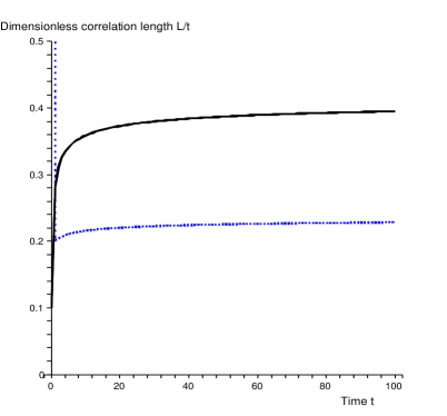
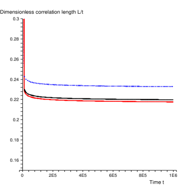
Fig. 14 shows the scaling density results of a model containing bound string states up to and . In agreement with Ref. Tye et al. (2005) the string densities of heavier states fall rapidly as the string tension increases. This is because of equation (44), which tends to give a small value of (hence a large value of ) for large ’s and ’s, so that heavy strings have the tendency to break to lighter ones. It is therefore possible to obtain a very good approximation of such a network by truncating the equations at a relatively low , like, in this case, . As one reduces the intercommuting probability (Fig. 14) string densities increase, as expected, and the fall of density with increasing string tension becomes more prominent. The relative importance of light to heavier string states depends on both the string coupling (appearing in the string tensions and ), and the intercommuting probability absorbed in ’s and ’s. However, the generic behaviour is that the string number density is dominated by strings of type , and , all having comparable number densities, while higher composite states are heavily suppressed.
The fact that the number density of the first bound state is comparable to that of the unbound strings can be understood in terms of the difference in string tension between F- and D-strings. This makes it energetically favourable for the light strings to be in a bound state. One can then envisage such a network as being predominantly composed by a heavy component of D-strings, together with a ‘cobweb’ of light F-strings, which tend to stick to the D-string network, giving rise to another heavy FD-string component.
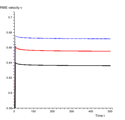
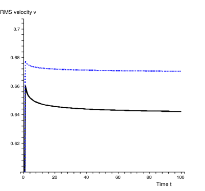
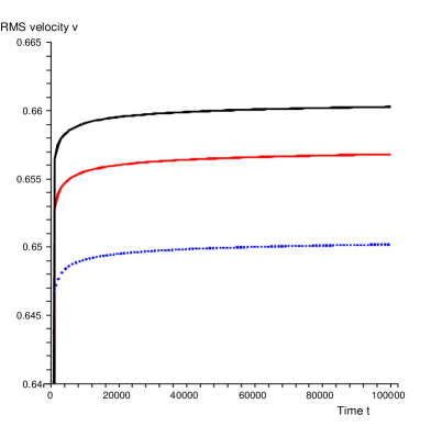
In our velocity dependent model we separately evolve the rms velocities of each string component of the network, which, since each string type has a different correlation length, can be significantly different. This is shown in Fig. 15 where, evidently, the less abundant strings also have smaller velocities. This could in principle be observable as the velocity enters the temperature discontinuity through the Kaiser-Stebbins effect Kaiser and Stebbins (1984); Vilenkin and Shellard (1994).
The above results provide further evidence in favour of the possibility of scaling in cosmic superstring networks and other ‘entangled’ networks with junctions. Particularly interesting is the fact that the scaling solutions we found do not rely on any additional energy damping mechanism, apart from loop production through self-intersections of strings. Indeed, by imposing energy conservation during zipping events, we have ensured that no energy is damped during the zipping processes, which would facilitate the reaching of a scaling regime. Possible non-elasticity of the zipping events would provide an additional decay channel, which would therefore further support our scaling results. One should keep in mind that the models we presented here and applied to the case of cosmic superstrings, are phenomenological in nature and, as such, do not model in detail a number of microphysical processes, related, for example, to the dynamics of string junctions Bettencourt et al. (1997) (see Ref. Rajantie et al. (2007) for recent field theory simulations). However, progress in understanding the complex, non-linear evolution of cosmic strings has been possible with the combination of different approaches (microphysical models, Nambu-Goto and field theory simulations, phenomenological models), and there is already strong evidence that models like those presented here capture most of the relevant physics. Being able to construct such analytic models of multi-tension string evolution and come up with quantitative predictions is an important step in our understanding of non-abelian cosmic (super)string evolution. It would be interesting to combine these models with other approaches to cosmic superstring modelling as for example field theory models Copeland and Saffin (2005); Saffin (2005); Hindmarsh and Saffin (2006) or Nambu-Goto multi-tension simulations.
VI Conclusion
We have presented analytic velocity-dependent models for the cosmological evolution of non-abelian string networks. Apart from ordinary abelian intercommutations, these models account for interactions between different string types, producing Y-type junctions with linking segments stretching between the originally colliding strings. We have described such interactions in terms of two limiting cases, namely zipper-type interactions, where the link is produced by the zipping of the colliding strings into a bound state, and bridge-type ones, where the link is a newly formed string of a third type and the parent strings do not lose significant string length. A general Y-junction forming interaction can be describing by a combination of these two inter-related mechanisms, and the relative weighting depends on the type of strings under study. In non-abelian field theory, where the interactions are topologically constrained, one can argue that the bridge-type picture is a good approximation as the colliding strings do not gain energy by converting length to the new type. On the other hand the zipper interaction corresponds closely to the case of cosmic superstrings, where D-strings and F-strings tend to bind together to form heavier composites.
In the bridge case, we have applied our models to the evolution of string networks and found that the presence of Y-type junctions does not generally lead to string frustration. Instead, scaling solutions exist for a wide range of physically relevant choices of parameters. Here, we have thus discussed the physical properties and scaling behaviour of networks for noting the same qualitative behaviour.
In the zipper case, we have modelled a cosmic superstring network as one consisting of two types of elementary strings (corresponding to F- and D-strings) which can zip together to form bound states between strings of one type and strings of the other. We have demonstrated scaling of all string types, with heavier strings generally less populated than lighter ones, as noted in Ref. Tye et al. (2005). We have also obtained the scaling velocities of each network component, with heavier strings moving slower than lighter ones. The general picture emerging from this analysis, is a string network whose number density is dominated by the lightest (unbound) strings and the first bound state between them, with all heavier bound states being suppressed. The first bound state develops a comparable number density to the unbound strings, even though it has a higher string tension. This is to be understood in terms of the difference in string tension between F- and D-strings, which makes it energetically favourable for the lightest F-strings to be in a bound FD-state. Thus, a scaling superstring network is dominated by D-strings and the first FD bound state, with a cobweb of lighter F-strings of comparable number density, but subdominant energy density.
The strength of our scaling results stems from the fact that we have not allowed additional energy damping processes associated to the production of junctions (though our models can accomodate these possibilities also), as we have enforced energy conservation in the relevant string interaction events. Thus, first, we can be sure that we are not observing a ‘spurious’ scaling behaviour due to artificially throwing away some of the energy involved, and, second, our scaling results provide evidence that loop production alone may be sufficient for scaling (even in the presence of junctions) without the necessity of extra energy losses, as for example massive radiation at zipping. However, it should be highlighted that our findings provide evidence, rather than proof, of scaling in such networks. Indeed, our models are phenomenological in nature and, as such, have their own limitations. In particular, the detailed microphysics of junctions, for example the possibility of unzipping, is not modelled explicitly, but only statistically and indirectly, through choices of the relevant parameters. In principle, if juncion dynamics is sufficiently complicated, these coefficients could inherit time dependence, a possibility we have not considered. One should therefore combine our results with other complementary approaches to this difficult problem, each of which captures only part of the relevant physics. What is encouraging, is that all complementary approaches seem to independently point towards scaling in these networks.
It would be interesting to compare these models to field theory simulations Copeland and Saffin (2005); Saffin (2005); Hindmarsh and Saffin (2006) and see whether quantitative agreement can be established. It would also be desirable to generalise them to include a second length-scale for each network component, as, for small intercommuting probabilities likely to appear in cosmic superstring networks, a two-scale VOS model (see also Ref. Austin et al. (1993) for a three-scale model) is needed in order to match Nambu-Goto simulations of single string networks Avgoustidis and Shellard (2006). Other variants of our models could also be constructed. For example, the models presented here assume that the production of junctions can be approximated by the two mechanisms described in Ref. McGraw (1998), namely the ‘zipper’, where the string lengths lost from each of the zipping strings equal the length of the produced link, and the ‘bridge’, where the lengths of the colliding strings are preserved. Recent studies of junction formation based on the Nambu-Goto action Copeland et al. (2006a, b) suggest a slightly different mechanism where strings lose or gain length subject to a constraint, which the vertex has to satisfy. This mechanism could be readily accommodated in our models. It is an interesting question to what extent scaling results depend on such choices. Analytic models like these will be useful in comparing and contrasting with other approaches to ‘entangled’ network evolution. Although quantitative agreement with numerical simulations has not yet been investigated, these models provide further evidence that scaling behaviour in networks with junctions is possible, if not generic.
Acknowledgements.
We would like to thank Carlos Martins for many fruitful conversations and valuable suggestions. We also thank Alkistis Pourtsidou for pointing out a typographical mistake on the Hubble expansion term of the string density equations, which was corrected in the current version. This work has also benefited from discussions with Ed Copeland and Anne Davis. A.A. acknowledges financial support from the Cambridge European Trust, the Cambridge Newton Trust and the European Network on Random Geometry (ENRAGE). This work was also supported by PPARC.Appendix A Parameter matrices for strings,
In this appendix we explore the topologically allowed outcomes from string collisions in the case of , , and networks.
A.1 strings
Consider with generator and elements . There are three types of string (say type 1, 2 and 3) corresponding to the non-trivial group elements , and respectively. We have so that strings of type 1 can produce a type 2 segment when they interact, that is
| (46) |
Thus, the crossing of two type 1 strings can have two different outcomes, as shown:
![[Uncaptioned image]](/html/0705.3395/assets/x30.png)
Similarly, we have: corresponding to
![[Uncaptioned image]](/html/0705.3395/assets/x31.png)
meaning that two incoming type 2 strings can end on a vertex and so the interaction between type 2 strings can then have two outcomes:
![[Uncaptioned image]](/html/0705.3395/assets/x32.png)
which is as in the first diagram,
and:
that is a type 1 and and a type 3 strings can end on a vertex, and can be treated as being the same string type with opposite orientation:
![[Uncaptioned image]](/html/0705.3395/assets/x33.png)
Hence there are only two distinct types of string, type and , with type being self-conjugate. The parameter matrix corresponding to the above interactions is (see also section IV.1):
| (47) |
A.2 strings
For we have . Associating a string type to each non-trivial generator, as before, we have:
Again, there are two types of string with interaction diagrams:
![[Uncaptioned image]](/html/0705.3395/assets/x34.png)
![[Uncaptioned image]](/html/0705.3395/assets/x35.png)
![[Uncaptioned image]](/html/0705.3395/assets/x36.png)
![[Uncaptioned image]](/html/0705.3395/assets/x37.png)
These are described by the parameter matrix:
| (48) |
Note that there is no self-conjugate string in this case.
A.3 strings
For we have . Now:
Some of the new diagrams arising are:
![[Uncaptioned image]](/html/0705.3395/assets/x38.png)
and:
![[Uncaptioned image]](/html/0705.3395/assets/x39.png)
There are only three string types with parameter matrix:
| (49) |
String is self-conjugate.
A.4 strings
For we have . Working as before:
Again, there are only three string types, but no self-conjugate strings. The parameter matrix is now:
| (50) |
References
- Albrecht et al. (1997) A. Albrecht, R. A. Battye, and J. Robinson, Phys. Rev. Lett. 79, 4736 (1997), eprint astro-ph/9707129.
- Albrecht et al. (1999) A. Albrecht, R. A. Battye, and J. Robinson, Phys. Rev. D59, 023508 (1999), eprint astro-ph/9711121.
- Dvali and Tye (1999) G. Dvali and S. H. H. Tye, Phys. Lett. B450, 72 (1999), eprint hep-ph/9812483.
- Burgess et al. (2004) C. P. Burgess, J. M. Cline, H. Stoica, and F. Quevedo, JHEP 09, 033 (2004), eprint hep-th/0403119.
- Kachru et al. (2003) S. Kachru, R. Kallosh, A. Linde, J. Maldacena, L. McAllister, and S. P. Trivedi, JCAP 0310, 013 (2003), eprint hep-th/0308055.
- Jeannerot et al. (2003) R. Jeannerot, J. Rocher, and M. Sakellariadou, Phys. Rev. D68, 103514 (2003), eprint hep-ph/0308134.
- Sazhin et al. (2003) M. Sazhin et al., Mon. Not. Roy. Astron. Soc. 343, 353 (2003), eprint astro-ph/0302547.
- Sazhin et al. (2004) M. V. Sazhin et al. (2004), eprint astro-ph/0406516.
- Schild et al. (2004) R. E. Schild, I. S. Masnyak, B. I. Hnatyk, and V. I. Zhdanov, Astron. Astrophys. 422, 477 (2004), eprint astro-ph/0406434.
- Lo and Wright (2005) A. S. Lo and E. L. Wright (2005), eprint astro-ph/0503120.
- Kibble (2004) T. W. B. Kibble (2004), eprint astro-ph/0410073.
- Polchinski (2004) J. Polchinski (2004), eprint hep-th/0412244.
- Davis and Kibble (2005) A. C. Davis and T. W. B. Kibble, Contemp. Phys. 46, 313 (2005), eprint hep-th/0505050.
- Majumdar (2005) M. Majumdar (2005), eprint hep-th/0512062.
- Battye et al. (2006) R. A. Battye, B. Garbrecht, and A. Moss, JCAP 0609, 007 (2006), eprint astro-ph/0607339.
- Bevis et al. (2007) N. Bevis, M. Hindmarsh, M. Kunz, and J. Urrestilla (2007), eprint astro-ph/0702223.
- Dvali et al. (2001) G. Dvali, Q. Shafi, and S. Solganik (2001), eprint hep-th/0105203.
- Burgess et al. (2001) C. P. Burgess, M. Majumdar, F. Quevedo, G. Rajesh, and R.-J. Zhang, JHEP 0107, 047 (2001), eprint hep-th/0105204.
- Garcia-Bellido et al. (2002) J. Garcia-Bellido, R. Rabadan, and F. Zamora, JHEP 01, 036 (2002), eprint hep-th/0112147.
- Jones et al. (2002) N. Jones, H. Stoica, and S. H. H. Tye, JHEP 0207, 051 (2002), eprint hep-th/0203163.
- Sarangi and Tye (2002) S. Sarangi and S. H. H. Tye, Phys. Lett. B536, 185 (2002), eprint hep-th/0204074.
- Dvali and Vilenkin (2004) G. Dvali and A. Vilenkin, JCAP 0403, 010 (2004), eprint hep-th/0312007.
- Copeland et al. (2004) E. J. Copeland, R. C. Myers, and J. Polchinski, JHEP 06, 013 (2004), eprint hep-th/0312067.
- Babichev and Kachelriess (2005) E. Babichev and M. Kachelriess, Phys. Lett. B614, 1 (2005), eprint hep-th/0502135.
- Avgoustidis and Shellard (2005a) A. Avgoustidis and E. P. S. Shellard, JHEP 08, 092 (2005a), eprint hep-ph/0504049.
- Brax et al. (2006) P. Brax, C. van de Bruck, A. C. Davis, and S. C. Davis, Phys. Lett. B640, 7 (2006), eprint hep-th/0606036.
- Melkumova et al. (2006) E. Y. Melkumova, D. V. Gal’tsov, and K. Salehi (2006), eprint hep-th/0612271.
- Jones et al. (2003) N. T. Jones, H. Stoica, and S. H. H. Tye, Phys. Lett. B563, 6 (2003), eprint hep-th/0303269.
- Jackson et al. (2005) M. G. Jackson, N. T. Jones, and J. Polchinski, JHEP 10, 013 (2005), eprint hep-th/0405229.
- Avgoustidis and Shellard (2005b) A. Avgoustidis and E. P. S. Shellard, Phys. Rev. D71, 123513 (2005b), eprint hep-ph/0410349.
- McGraw (1998) P. McGraw, Phys. Rev. D57, 3317 (1998), eprint astro-ph/9706182.
- Vilenkin and Shellard (1994) A. Vilenkin and E. P. S. Shellard, Cosmic Strings and Other Topological Defects (Cambridge University Press, 1994).
- Spergel and Pen (1997) D. Spergel and U.-L. Pen, Astrophys. J. 491, L67 (1997), eprint astro-ph/9611198.
- McGraw (1996) P. McGraw (1996), eprint hep-th/9603153.
- Kibble (1985) T. W. B. Kibble, Nucl. Phys. B252, 227 (1985).
- Bennett (1986) D. Bennett, Phys. Rev. D33, 872 (1986).
- Albrecht and Turok (1989) A. Albrecht and N. Turok, Phys. Rev. D40, 973 (1989).
- Allen and Shellard (1990) B. Allen and E. P. S. Shellard, Phys. Rev. Lett. 64, 119 (1990).
- Martins and Shellard (2002) C. J. A. P. Martins and E. P. S. Shellard, Phys. Rev. D65, 043514 (2002), eprint [http://arXiv.org/abs]hep-ph/0003298.
- Martins (2004) C. J. A. P. Martins, Phys. Rev. D70, 107302 (2004), eprint hep-ph/0410326.
- Tye et al. (2005) S. H. H. Tye, I. Wasserman, and M. Wyman, Phys. Rev. D71, 103508 (2005), eprint astro-ph/0503506.
- Copeland and Saffin (2005) E. J. Copeland and P. M. Saffin, JHEP 11, 023 (2005), eprint hep-th/0505110.
- Copeland et al. (2006a) E. J. Copeland, T. W. B. Kibble, and D. A. Steer, Phys. Rev. Lett. 97, 021602 (2006a), eprint hep-th/0601153.
- Copeland et al. (2006b) E. J. Copeland, T. W. B. Kibble, and D. A. Steer (2006b), eprint hep-th/0611243.
- Saffin (2005) P. M. Saffin, JHEP 09, 011 (2005), eprint hep-th/0506138.
- Hindmarsh and Saffin (2006) M. Hindmarsh and P. M. Saffin, JHEP 08, 066 (2006), eprint hep-th/0605014.
- Avelino et al. (2006) P. P. Avelino, C. J. A. P. Martins, J. Menezes, R. Menezes, and J. C. R. E. Oliveira, Phys. Rev. D73, 123520 (2006), eprint hep-ph/0604250.
- Bennett and Bouchet (1990) D. Bennett and F. Bouchet, Phys. Rev. D41, 2408 (1990).
- Shellard (1987) E. P. S. Shellard, Nucl. Phys. B283, 624 (1987).
- Matzner and Mccracken (1988) R. A. Matzner and J. Mccracken (1988), in *NEW HAVEN 1988, PROCEEDINGS, COSMIC STRINGS* 32-41.
- Hanany and Hashimoto (2005) A. Hanany and K. Hashimoto, JHEP 06, 021 (2005), eprint hep-th/0501031.
- Martins and Shellard (1996a) C. J. A. P. Martins and E. P. S. Shellard, Phys. Rev. D53, 575 (1996a), eprint [http://arXiv.org/abs]hep-ph/9507335.
- Martins and Shellard (1996b) C. J. A. P. Martins and E. P. S. Shellard, Phys. Rev. D54, 2535 (1996b), eprint [http://arXiv.org/abs]hep-ph/9602271.
- Allen and Caldwell (1990) B. Allen and R. Caldwell, Phys. Rev. Lett. 65, 1705 (1990).
- Austin (1993) D. Austin, Phys. Rev. D48, 3422 (1993).
- Embacher (1992) F. Embacher, Nucl. Phys. B387, 129 (1992).
- Austin et al. (1993) D. Austin, E. J. Copeland, and T. W. B. Kibble, Phys. Rev. D48, 5594 (1993), eprint [http://arXiv.org/abs]hep-ph/9307325.
- Martins (1997) C. J. A. P. Martins (1997), PhD Thesis, University of Cambridge.
- Moore et al. (2002a) J. N. Moore, E. P. S. Shellard, and C. J. A. P. Martins, Phys. Rev. D65, 023503 (2002a), eprint hep-ph/0107171.
- Achucarro and de Putter (2006) A. Achucarro and R. de Putter, Phys. Rev. D74, 121701 (2006), eprint hep-th/0605084.
- Alford et al. (1992) M. G. Alford, K.-M. Lee, J. March-Russell, and J. Preskill, Nucl. Phys. B384, 251 (1992), eprint hep-th/9112038.
- Bucher (1991) M. Bucher, Nucl. Phys. B350, 163 (1991).
- Wilczek and Wu (1990) F. Wilczek and Y.-S. Wu, Phys. Rev. Lett. 65, 13 (1990).
- Toulouse (1976) G. Toulouse, J. Physique Lett. 38 (1976).
- Mermin (1979) N. Mermin, Reviews of Modern Physics 51, 625 (1979).
- Aryal et al. (1986) M. Aryal, A. E. Everett, A. Vilenkin, and T. Vachaspati, Phys. Rev. D34, 434 (1986).
- Vachaspati and Vilenkin (1987) T. Vachaspati and A. Vilenkin, Phys. Rev. D35, 1131 (1987).
- Bettencourt and Kibble (1994) L. M. A. Bettencourt and T. W. B. Kibble, Phys. Lett. B332, 297 (1994), eprint hep-ph/9405221.
- Moore et al. (2002b) J. N. Moore, E. P. S. Shellard, and C. J. A. P. Martins, Phys. Rev. D65, 023503 (2002b), eprint hep-ph/0107171.
- Vincent et al. (1997) G. R. Vincent, M. Hindmarsh, and M. Sakellariadou, Phys. Rev. D56, 637 (1997), eprint astro-ph/9612135.
- Hindmarsh and Kibble (1985) M. Hindmarsh and T. W. B. Kibble, Phys. Rev. Lett. 55, 2398 (1985).
- Aryal and Everett (1987) M. Aryal and A. E. Everett, Phys. Rev. D35, 3105 (1987).
- Kaiser and Stebbins (1984) N. Kaiser and A. Stebbins, Nature 310, 391 (1984).
- Bettencourt et al. (1997) L. M. A. Bettencourt, P. Laguna, and R. A. Matzner, Phys. Rev. Lett. 78, 2066 (1997), eprint hep-ph/9612350.
- Rajantie et al. (2007) A. Rajantie, M. Sakellariadou, and H. Stoica, JCAP 0711, 021 (2007), eprint 0706.3662.
- Avgoustidis and Shellard (2006) A. Avgoustidis and E. P. S. Shellard, Phys. Rev. D73, 041301 (2006), eprint astro-ph/0512582.
- Firouzjahi et al. (2006) H. Firouzjahi, L. Leblond, and S. H. Henry Tye, JHEP 05, 047 (2006), eprint hep-th/0603161.
- Leblond and Wyman (2007) L. Leblond and M. Wyman (2007), eprint astro-ph/0701427.
- Avgoustidis (2008) A. Avgoustidis, Phys. Rev. D78, 023501 (2008), eprint 0712.3224.