Vacuumless kinks systems from vacuum ones, an example

Abstract

Some years ago, Cho and Vilenkin, introduced a model which presents topological solutions, despite not having degenerate vacua as is usually expected. Here we present a new model with topological defects, connecting degenerate vacua but which in a certain limit recovers precisely the one proposed originally by Cho and Vilenkin. In other words, we found a kind of “parent” model for the so called vacuumless model. Then the idea is extended to a model recently introduced by Bazeia et al. Finally, we trace some comments the case of the Liouvlle model.

PACS: 11.10.Lm, 11.27.+d

Usually the topological objects like domain walls, strings and monopoles appears when the models support at least two degenerate vacua. Notwithstanding, there are some models which defy this commonsense, like the Liouville model [1] - [3], the vacuumless (VL) model introduced originally by Cho and Vilenkin [4] - [6] and, more recently a model where the kink interpolates between two inflection points instead vacua [7]. Here we are going to concentrate our attention to the VC case, which was originally studied regarding gravitational aspects of the topological defect [4], and then regarding its topological properties [5], and after that make a discussion in general lines about how to implement a similar procedure in the other two cited cases. The Lagrangian density of the model we are going to introduce here is the usual one for a scalar field,

$$\mathcal{L}=\frac{1}{2}\partial_{\mu}\varphi\partial^{\mu}\varphi\,-\,V\left(\varphi\right)$$ (1)

where the potential is given by

$$V\left(\varphi\right)=\frac{1}{2}\left(Acosh(\varphi)-Bsech(\varphi)\right)^{2}.$$ (2)

Note that, if $A=0$ and $B=\pm\,\mu$, we recover the usual vacuumless potential [5]

$$V\left(\varphi\right)=\frac{\mu^{2}}{2}\left(sech(\varphi)\right)^{2}.$$ (3)

Let us use the BPS approach [8], in order to present the solution of this and the new model we introduced above. For this, one can write the potential in terms of the so called superpotential, which is given by

$$\,V\left(\phi\right)=\frac{1}{2}\,W_{\phi}^{2},$$ (4)

from which the energy of the static configuration can be obtained as

$$E_{BPS}=\frac{1}{2}\int_{-\infty}^{\infty}dx\left[\left(\frac{d\phi}{dx}-W_{\phi}\right)^{2}+W_{\phi}\frac{d\phi}{dx}\right].$$ (5)

Observing this equation, we note that the field configuration which minimizes the energy will obeys the first-order differential equation

$$\frac{d\phi}{dx}=W_{\phi}\left(\phi\right),$$ (6)

and his energy is written as

$$E_{BPS}=|W\left(\phi\left(\infty\right)\right)-W\left(\phi\left(-\infty\right)\right)|.$$ (7)

Let us now apply this machinery to the above mentioned models. In the case of the VL model, one can check that the superpotential is given by [5]

$$W\left(\phi\right)=2\,B\,\tan^{-1}\left[\tan\left(\frac{\phi}{2}\right)\right],$$ (8)

and its slowly divergent kink looks like

$$\phi\left(x\right)=\sinh^{-1}\left(B\,\,x\right).$$ (9)

On the other hand, in the case of the model which we are introducing here (2), the superpotential has the appearance

$$W\left(\phi\right)=A\,\sinh\left(\phi\right)-2\,B\,\tan^{-1}\left[\tan\left(\frac{\phi}{2}\right)\right],$$ (10)

and the corresponding kink and antikink are expressed as

$$\phi\left(x\right)=\pm\,\sinh^{-1}\left[\sqrt{\frac{\left(A-B\right)}{A}}\,\tan\left(\sqrt{A\left(A-B\right)}\,\,x\right)\right],$$ (11)

from which it can be verified that the expected limit (9) when $A\rightarrow 0$ is really achieved. It is possible to observe too, from the Figure 1, that when $A\rightarrow 0$ the vacua of the model becomes more and more far from each other, in such a way that one can think the VL model [4], as a limit of this model with usual degenerate vacua. Once in this case, the limit of the field configuration at $x\rightarrow\pm\,\infty$, are the vacua of the model, we can assure that in these limits, the field given in (11) goes to

$$\phi\left(\pm\infty\right)=\pm\,\cosh^{-1}\left(\sqrt{\frac{B}{A}}\right).$$ (12)

Note that, for consistency, the model will have two minima provided that $B>A$, otherwise the potential has only one minimum and the solution of the equation (11) presents singularities at finite points in the space, so rendering itself as a nonphysical solution. The BPS energy of this configuration will then be given by

$$E_{BPS}\left(A,B\right) = 2\,\left|\left(A+\sqrt{A\,B}\right)\sqrt{\frac{A+B-2\sqrt{A\,B}}{B-A}+}\right.$$

$$\left.-2\,B\,\tan^{-1}\left[\tanh\left(\frac{1}{2}\cosh^{-1}\left(\sqrt{\frac{B}{A}}\right)\right)\right]\right|.$$

Let us now analyze the limit of this energy when $A\rightarrow 0$. The first term vanishes obviously, and in the second we see that the argument of the function diverges and, as we know, the inverse function of the hyperbolic cosine diverges too, but the hyperbolic tangent of infinity is simply one. As a consequence we conclude that the limit of the above energy is simply given by

$$E_{BPS}\left(0,B\right)=\,\pi\,B,$$ (14)

which is in absolute accordance with the expected for the VL model [5]. The energy density of the model we are studying is

$$\varepsilon\left(x\right)=\frac{\left(A-B\right)^{2}\sec\left(\sqrt{A\left(A-B\right)\,x}\right)^{4}}{\left(1+(1-B/A)\tan\left(\sqrt{A\left(A-B\right)\,x}\right)^{2}\right)},$$ (15)

and, as expected, have the correct limit when $A\rightarrow 0$, becoming itself equal to that of the VL model

$$\varepsilon\left(x\right)=\frac{B^{2}}{\left(1+B^{2}x^{2}\right)},$$ (16)

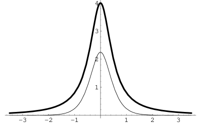
Figure 2: The energy density dependence in $x$ when $B=2$ and $A=0.5$ (thin line) and the vaccumless case.

but for a fixed value of the parameter $B$, the VL model have a bigger and less concentrated energy density, as can be seen in the Figure 2. Now, we can discuss the linear stability of the model here presented. In fact, as shown in [9] for the case of coupled scalar fields, the linear stability of the model with one scalar field can be done as usual by performing small perturbations on the kink solution,

$$\phi\left(x,t\right)=\phi_{kink}\left(x\right)+\eta\left(x,t\right).$$ (17)

Taking into account only up to the first order terms in the perturbation, which leads to a Schroedinger-like equation for the perturbation field

$$\left(-\frac{d^{2}}{dx^{2}}+V_{\phi\phi}\left(\phi\equiv\phi_{kink}\left(x\right)\right)\right)\eta_{n}\left(x\right)=\omega_{n}^{2}\,\eta_{n}\left(x\right),$$ (18)

where $\eta\left(x,t\right)\equiv\sum_{n}\,\eta_{n}\left(x\right)\,\cos\left(\omega_{n}\,t\right)$. It is not difficult to see that the above equation can be achieved from the following ladder operators,

$$a_{\pm}\equiv\pm\,\frac{d}{dx}+W_{\phi\phi},$$ (19)

whose Hamiltonian operator $\hat{H}=a_{+}\,a_{-}$, as shown in [10] for general coupled real scalar fields, have their eigenvalues positive definite and, as a consequence, the models are stable under small quantum fluctuations.

In our case, the potential to which the small fluctuations feel, once again has the VL one as its limit, coming from above as can be observed in Figure 3.

The bosonic ground stated, which is granted by the translational invariance in this case, in general can be obtained through the solution of the equation,

$$\left(-\frac{d}{dx}+W_{\phi\phi}\right)\psi_{0}\left(x\right)=0,$$ (20)

where, as a simplified notation, from now on we define that $W_{\phi\phi}\equiv W_{\phi\phi}\left(\phi\equiv\phi_{kink}\right)$. Here we note that, one can rewrite the above equations as

$$\frac{d\psi_{0}\left(x\right)}{\psi_{0}\left(x\right)}=W_{\phi\phi}\,dx,$$ (21)

but we know from the BPS equation that $dx=\frac{d\phi}{W_{\phi}}$, in such a way that a direct relation between the bosonic zero-mode and the superpotential can be obtained,

$$\psi_{0}\left(x\right)=N_{0}\,W_{\phi}=N_{0}\,\frac{\sqrt{A}\left(A-B\right)\left(\sec\left(\sqrt{A\left(A-B\right)}\,x\right)\right)^{2}}{\sqrt{1+\left(A-B\right)\left(\tan\left(\sqrt{A\left(A-B\right)}\,x\right)\right)^{2}}},$$ (22)

where $N_{0}$ is the normalization constant, and his shape is quite similar to that of the VL model. This allow us to show that the normalization of the zero-mode is related to the BPS energy through

$$\int\left|\psi_{0}\left(x\right)\right|^{2}dx=N_{0}^{2}\int\,W_{\phi}^{2}\,dx=N_{0}^{2}\int\,W_{\phi}\,d\phi=N_{0}^{2}\,E_{BPS}\equiv 1,$$ (23)

and we get finally the normalized bosonic zero-mode

$$\psi_{0}\left(x\right)=\sqrt{\frac{1}{E_{BPS}}}\,W_{\phi},$$ (24)

apart from an arbitrary constant phase factor. Let us now try to calculate the fermionic zero-mode. Using in this case, as done by Bazeia in [5], the Yukawa coupling giving by $f\left(\phi\right)\,\bar{\psi}\,\psi$, where it is chosen $f\left(\phi\right)=g\,W_{\phi\phi}$ ($g=1$, in order to get a supersymmetric version of the model [11]), we reach the following equation for Dirac fermions

$$i\,\gamma^{1}\frac{d\Psi}{dx}+f\left(\phi\right)\,\Psi=0,\,\Psi=\left(\begin{array}[]{l}\psi_{+}\\ \psi_{-}\end{array}\right),$$ (25)

and using the representation where $i\,\gamma^{1}\rightarrow\sigma_{3}$ we obtain the following equations for the spinor components,

$$\pm\,\frac{d\psi_{\pm}}{dx}+f\left(\phi\right)\psi_{\pm}=0.\,$$ (26)

The above equations can be expressed as

$$\frac{d\psi_{\pm}}{\psi_{\pm}}=\mp f\left(\phi\right)\,dx=\mp g\,W_{\phi\phi}\,\frac{d\phi}{W_{\phi}},$$ (27)

which integration gives us finally the spinor

$$\Psi=\left(\begin{array}[]{l}C_{+}\,\,W_{\phi}^{-g}\\ C_{-}\,\,W_{\phi}^{g}\end{array}\right),$$ (28)

where $C_{\pm}$ are arbitrary integration constants. However, supposing that the function $W_{\phi}$ is well-behaved, vanishing when $x\rightarrow\pm\,\infty$. The normalization of the above spinor,

$$\int\left|\Psi\right|^{2}dx=\int dx\,\left[\left|C_{+}\right|^{2}\,\,W_{\phi}^{-2\,g}+\left|C_{-}\right|^{2}\,\,W_{\phi}^{2\,g}\right]\equiv 1,$$ (29)

will impose that one of the above arbitrary constants must be chosen equal to zero. Otherwise, the spinor will be not square integrable and, as a consequence, we are left with two possible solutions, depending on the signal of $g$,

$$\Psi_{+}=C_{+}\,\,W_{\phi}^{-g}\left(\begin{array}[]{l}1\\ 0\end{array}\right),\,g<0;\,\Psi_{\_}=C_{-}\,\,W_{\phi}^{g}\left(\begin{array}[]{l}0\\ 1\end{array}\right),\,g>0.$$ (30)

In fact, the normalizability of the spinor, implies into further conditions over the constant $g$. Let us return to the normalization integration, now simply given by

$$\int\left|\Psi_{\pm}\right|^{2}dx=\left|C_{\pm}\right|^{2}\,\int dx\,\,W_{\phi}^{\left(\mp 2\,g\right)}=\left|C_{\pm}\right|^{2}\int\,\,W_{\phi}^{\left(\mp 2\,g\,-1\right)}d\phi.$$ (31)

Once again, we note that $\left|g\right|\leq\frac{1}{2}$ or the integration may diverge. At this point, however, some differences can appear depending which model is being considered. In order to be quite clear on this point, let us take for instance the limiting case $g=\pm\frac{1}{2}$, where we have

$$\left|C_{\pm}\right|^{2}\int\,\,W_{\phi}^{\left(\mp 2\,g\,-1\right)}d\phi=\left|C_{\pm}\right|^{2}\int\,d\phi=\left|C_{\pm}\right|^{2}\left(\phi\left(+\infty\right)-\phi\left(\infty\right)\right).$$ (32)

It is evident that in models like the VL, the zero-mode fermion can not be normalizable, due to the divergence of the kink profile [5]. However, for any usual topological model with different finite vacua, this case is absolutely admissible. So, the model we have proposed in this work, can have its fermionic zero-mode well defined for any value of the parameter $A$ different of zero, when it becomes equivalent to the VL model. So, we can think this model as a kind of regularizing potential, where one can make the vacua arbitrarily far from each other, without losing the finiteness characteristic of the usual BPS kinks. In fact, in the VL limit, the normalization constant tends to zero and the zero mode wave function vanishes. Only in the VL limit the $g=\pm 1/2$ must be avoided.

Now, considering the cases where a supersymmetric extension of the model is allowed [11], $g=\pm 1$. The normalization of the fermionic zero-mode, becomes quite similar to that of its bosonic counterpart,

$$C_{\pm}=\sqrt{\frac{1}{E_{BPS}}}.$$ (33)

Let us now briefly discuss the extension of this idea to other unusual kink models. For instance we take as our next example, the model introduced recently by Bazeia, Losano and Malbouisson (BLM) [7]. This model is unbounded from below and presents no vacua, just a maximum at the origin. Notwithstanding, it has a kink (and antikink) connecting their two inflection points. Concretely, his potential is given by

$$V_{BLM}\left(\phi\right)=\frac{1}{2}\left(1-\phi^{2}\right)^{3}.$$ (34)

Following the idea above introduced, we now propose an alternative model which presents two local minima. In fact it is not yet a standard one, once it is also unbounded from bellow. For this case the “parent” model is defined as

$$V_{P}\left(\phi\right)=\frac{1}{2}\left(1-\phi^{2}\right)\left(A-1+\phi^{2}\right)^{2}.$$ (35)

Both potentials are plotted in Figure 4. Once again, when one takes the limit $A\rightarrow 0$, the BLM model is recovered. Again there is no problem in consider $g=\pm\frac{1}{2}$, when calculating the fermionic zero mode. The kink solution of the parent model in this case is given by

$$\phi\left(x\right)=\pm\,\tanh\left\{\sinh^{-1}\left[\sqrt{\frac{\left(A-1\right)}{A}}\,\tan\left(\sqrt{A\left(A-1\right)}\,\,x\right)\right]\right\}.$$ (36)

In fact this is nothing but the deformation of the first model proposed here, precisely in the same way in which the BLM model can be viewed as a deformation of the VC model [7].

Finally, let us make a brief comment about the case of the Liouville model, where

$$V\left(\phi\right)=\left(\frac{m}{\beta}\right)^{2}e^{\beta\,\phi},$$ (37)

which evidently does not presents any vacuum. It is possible to create a model composing a series of exponential factors, in such a way that we could have a “parent” model also here. However, at least this simple extension is not exactly solvable. In this case only a numerical solution is available in principle, and we are not going to consider it.

Our last comment in this work, is that we think that it is possible to find orthodox “parent” kink models for those which unorthodox features, like the VL, BLM and Liouville models. At least when is is possible, as shown in the case of the VL model here, we get a kind of regularization of the kink properties, softening some of his properties.

Acknowledgments: The authors are grateful to CNPq and CAPES for partial financial support, and ASD to the Professor D. Bazeia for introducing him to this matter. This work has been finished during a visit (ASD) within the Associate Scheme of the Abdus Salam ICTP.

Figure 1: The potential as a function of the scalar field $\varphi$. A typical profile for $A$ significantly different of zero (thin line) and when $A$ is close to zero.

Figure 3: The potential of the Scroedinger-like stability equation as a function of the spatial variable, both in the case of potential with degenerate vacua (thin line, $A=0.9$, $B=1$) as in the vacuumless case.

Figure 4: The potential as a function of the scalar field $\varphi$. A typical profile for $A$ significantly different of zero and for the BLM model (thin line).

References

- [1] E. D’Hoker and R. Jackiw, Phys. Rev. D 26 (1982) 3517; Phys. Rev. Lett. 50 (1982) 1719.
- [2] E. D’Hoker, D. Z. Freedman and R. Jackiw, Phys. Rev. D 28 (1982) 2583.
- [3] P. Menotti and G. Vajente, Nucl. Phys. B 709 (2005) 465.
- [4] I. Cho and A. Vilenkin, Phys. Rev. D 59 (1999) 021701(R); 59 (1999) 063510.
- [5] D. Bazeia, Phys. Rev. D 60 (1999) 067705.
- [6] A. A. Sen, Int. J. Mod. Phys. D 10 (2001) 515.
- [7] D. Bazeia, L. Losano and J. M. C. Malbouisson, Phys. Rev. D 66 (2002) 101701(R).
-
[8]
M. K. Prasad and C. M. Sommerfield, Phys. Rev. Lett. 35 (1975) 760; E. B. Bolgomol ’nyi, Sov. J. Nucl. Phys.
24 (1976) 449.
- [9] D. Bazeia, R. F. Ribeiro and M. M. Santos, Phys. Rev. E 54 (1996) 2943.
- [10] D. Bazeia, M. M. Santos, Phys. Lett. A 217 (1996) 28.
- [11] B. Chibisov and M. Shifman, Phys. Rev. D 56 (1997) 7990.