Detecting anchoring in financial markets

Abstract

Anchoring is a term used in psychology to describe the common human tendency to rely too heavily (anchor) on one piece of information when making decisions. A trading algorithm inspired by biological motors, introduced by L. GilGil , is suggested as a testing ground for anchoring in financial markets. An exact solution of the algorithm is presented for arbitrary price distributions. Furthermore the algorithm is extended to cover the case of a market neutral portfolio, revealing additional evidence that anchoring is involved in the decision making of market participants. The exposure of arbitrage possibilities created by anchoring gives yet another illustration on the difficulty proving market efficiency by only considering lower order correlations in past price time series.

Keywords: Anchoring, behavioral finance, biological motors, trading algorithm, brownian motion

Behavioral finance has become a growingly influential subbranch of finance, stressing how human and social emotional biases can affect market prices. The field adapts a more pragmatic and complex view on financial markets, in contrast to standard finance theory where people rationally and independently on basis of full information try to maximize utility. The more realistic view comes at a cost however, since a multifactorial world is captured mainly via observations or postulates about human behavior.

One of the first observations of anchoring was reported in the now classical experiment by Tversky and KahnemanTversky . Two groups of test persons were shown to give different mean estimates of the percentage of African nations in the United Nations, depending on the specific anchor of percentage suggested by the experimenters to the two groups. Evidence for human anchoring has since been reported in many completely different domains such as e.g. customer inertia in brand switchingYe (old brand price act as an anchor), whereas other evidence come from studies on on-line auctionsDodonova (people bid more for an item the higher the “buy-now” price) and anchoring in real estate pricesNorthcraft (subjects appraisal values depend on arbitrary posted listing price of the house). In the context of financial markets anchoring has been observed via the so called “disposition effect”Shefrin ,Heilmann which is the tendency for people to sell assets that have gained value and keep assets that have lost value. As noted in Weber conclusive tests using real market data is usually difficult because the investors’ expectations, as well as individual decisions, can not be controlled or easily observed. In experimental security trading however subjects were observed to sell winners and keep losersWeber .

In order to get a more firm understanding of how aggregation of individual behavior can give rise to measurable effects in a population in general and financial markets in particular, it would be interesting to model specific human traits on a micro scale and study the emergence of a dynamics with observable or even predictable effects on a macro scale. The hope would be to reproduce in models many of the mechanisms reported at work in behavioral finance. One step in this direction was done in Andersen1 where it was shown how consensus (called “decoupling” in Andersen1 ) and thereby predictability could emerge due to mutual influence of the price in a commonly traded asset, among a group of agents who had initially different opinions. Here another method is suggested which rigourously test for a different human trait introduced by behavioral finance, namely anchoring. The algorithm used was introduced by L. Gil Gil , and is inspired from the way biological motors work by exploiting favourable brownian fluctuations to generate directed forces and move. Similar ideas were also introduced in Sornette where it was shown how increments of uncorrelated time series can be predicted with a universal 75% probability of success.

Specifically, assume an agent at every time step $t$ uses a fixed amount of his wealth to hold a long position in one out of $N$ assets. For simplicity $N=2$ will be used in the following, but the arguments can be extended to arbitrary $N$. Assume furthermore that the probability distribution functions (pdf’s) of the price of the two assets, $P_{1}(A_{1}),P_{2}(A_{2})$ are stationary distributions. Instead of the usual assumption of a random walk of the returns, short time anchoring of prices at quasi static price levels is imposed. No specific shape is assumed and the assets can be correlated or not, but any correlation is irrelevant for the following arguments. As noted in Gil the assumption of short term stationarity of prices can arise because of price reversal dynamics caused e.g. by monetary policies. As will be argued and tested for in the following , short term “stationarity” in prices can also be created due to short term human memory as to when an asset is “cheap” or “expensive”.

Consider any given instantaneous fluctuation of the prices $(A_{1},A_{2})$ around their quasi static price levels $(\bar{A_{1}},\bar{A_{2}})$. Classifying the $2^{N}$ different cases according whether $A_{i}<\bar{A_{i}}$ or $A_{i}>\bar{A_{i}}$, one has for $N=2$ the four different configurations $x_{i}$:

$x_{1}$	$x_{2}$	$x_{3}$	$x_{4}$
$A_{1}$ —	$A_{1}$ —
$\updownarrow dA_{1}$	$\updownarrow dA_{1}$
$\bar{A_{1}}$  ——-	$\bar{A_{1}}$  ——-	$\bar{A_{1}}$  ——-	$\bar{A_{1}}$  ——-
		$\updownarrow dA_{1}$	$\updownarrow dA_{1}$
		$A_{1}$ —	$A_{1}$ —
	$A_{2}$ —		$A_{2}$ —
	$\updownarrow dA_{2}$		$\updownarrow dA_{2}$
$\bar{A_{2}}$  ——-	$\bar{A_{2}}$  ——-	$\bar{A_{2}}$  ——-	$\bar{A_{2}}$  ——-
$\updownarrow dA_{2}$		$\updownarrow dA_{2}$
$A_{2}$ —		$A_{2}$ —

In steady state the probability flux into a given configuration $x_{i}$ equals the probability flux out of that configuration:

$$\sum_{j}P(x_{j})P(x_{j}\rightarrow x_{i}) = \sum_{j}P(x_{i})P(x_{i}\rightarrow x_{j})$$ (1)

The averaged return per time unit in the steady state, $R_{\rm av}$, is then given by

$$R_{\rm av} = \sum_{i=1}^{4}\sum_{j=1}^{4}P(x_{i})P(x_{i}\rightarrow x_{j})r_{\rm av}(x_{i}\rightarrow x_{j})$$ (3)

with $r_{\rm av}(x_{i}\rightarrow x_{j})$ the averaged return gained/lost in the transition $x_{i}\rightarrow x_{j}$. For each configuration $x_{i}$ one is assumed to hold a long position of either asset 1 or asset 2. Let $s=i$ be a state variable indicating that one is long one position of asset $i$. Then

$$r_{\rm av}(x_{i}\rightarrow x_{j}) = P(s=1|x_{i})r_{\rm av}(x_{i}\rightarrow x_{j}|s=1)+P(s=2|x_{i})r_{\rm av}(x_{i}\rightarrow x_{j}|s=2)$$ (4)

where $P(s=i|x_{j})$ denotes the probability holding asset $i$ given the knowledge to be in configuration $x_{j}$. $r_{\rm av}(x_{i}\rightarrow x_{j}|s=k)$ denotes the averaged return in steady state holding asset $k$ with a transition from configuration $x_{i}$ to $x_{j}$ and is given by:

$$r_{\rm av}(x_{j}\rightarrow x_{k}|s=k) = \int dA_{k}\int dA_{k}^{{}^{\prime}}\ln({A_{k}^{{}^{\prime}}\over A_{k}})P(A_{k}^{{}^{\prime}}|x_{i})P(A_{k}|x_{j})$$ (5)

$P(A_{k}|x_{i})$ denotes the probability to get the price $A_{k}$ conditioned on being in configuration $x_{i}$. For example knowing to be in configuration $x_{1}$ one has: $P(A_{2}|x_{1})={P(A_{2})\theta(A_{2}\leq 0)\over\int_{-\infty}^{0}P(A_{2}^{{}^{\prime}})dA_{2}{{}^{\prime}}}$ with $\theta(A_{2}\leq 0)$ a Heaviside function. Using (3-5) the general expression for the average return gained by the algorithm takes the form:

$$R_{\rm av} = \sum_{i=1}^{4}\sum_{j=1}^{4}\sum_{s=1}^{2}P(x_{i})P(x_{i}\rightarrow x_{j})P(s|x_{i})\int dA_{k}\int dA_{l}\ln({A_{l}\over A_{k}})P(A_{l}|x_{i})P(A_{k}|x_{j})$$ (6)

The corresponding risk measured by the averaged standard deviation of the return is given by:

$$\sigma^{2} = <(r-R_{\rm av})^{2}>$$ (7)

$$= \sum_{i=1}^{4}\sum_{j=1}^{4}\sum_{s=1}^{2}P(x_{i})P(x_{i}\rightarrow x_{j})P(s|x_{i})\int dA_{k}\int dA_{l}\ln({A_{l}\over A_{k}})^{2}P(A_{l}|x_{i})P(A_{k}|x_{j})-R_{\rm av}^{2}$$ (8)

The “trick” of the algorithm consists in breaking the symmetry by always choosing $P(s|x_{i})$ according to the following rules:

$$P(s=1|x_{1})=0;\ \ p(s=2|x_{1})=1; \ \ p(s=1|x_{2})=p(s=2|x_{2})=1/2;$$

$$P(s=1|x_{3})=p(s=2|x_{3})=1/2; \ \ p(s=1|x_{4})=1;\ \ p(s=2|x_{4})=0$$ (9)

That is, if not already long, one always take a long position of asset 2 (1) whenever configuration $x_{1}$ ($x_{4}$) happens, since the asset is undervalued in this case. Likewise if one is long of asset 1 (2) whenever configuration $x_{1}$ ($x_{4}$) happens one sell that asset since it is overvalued. To illustrate the algorithm consider the simplest case where $P(A_{i})$ take only two values $\bar{A_{i}}\pm dA_{i}$ with equal probability $1/2$. Inserting

$$P(A_{1}|x_{1})=\delta(\bar{A}_{1}+dA_{1});\ \ P(A_{1}|x_{2})=\delta(\bar{A}_{1}+dA_{1});\ \ P(A_{1}|x_{3})=\delta(\bar{A}_{1}-dA_{1});\ \ P(A_{1}|x_{4})=\delta(\bar{A}_{1}-dA_{1});$$

$$P(A_{2}|x_{1})=\delta(\bar{A}_{2}-dA_{2});\ \ P(A_{2}|x_{2})=\delta(\bar{A}_{2}+dA_{2});\ \ P(A_{2}|x_{3})=\delta(\bar{A}_{2}-dA_{2});\ \ P(A_{2}|x_{4})=\delta(\bar{A}_{2}+dA_{2})$$ (10)

and $P(x_{i})=P(x_{i}\rightarrow|x_{j})=1/4$ into (6) one gets the averaged return:

$$R_{\rm av}^{\bar{A_{i}}\pm dA_{i}} = 1/8\ \ [\ln({\bar{A}_{1}+dA_{1}\over\bar{A}_{1}-dA_{1}})+\ln({\bar{A}_{2}+dA_{2}\over\bar{A}_{2}-dA_{2}})]$$ (11)

with a variance given by

$$(\sigma_{\rm av}^{\bar{A_{i}}\pm dA_{i}})^{2} = 15/64\ln^{2}({\bar{A}_{1}+dA_{1}\over\bar{A}_{1}-dA_{1}})+15/64\ln^{2}({\bar{A}_{2}+dA_{2}\over\bar{A}_{2}-dA_{2}})-1/32\ln({\bar{A}_{2}+dA_{2}\over\bar{A}_{2}-dA_{2}}{\bar{A}_{1}+dA_{1}\over\bar{A}_{1}-dA_{1}})$$ (12)

Figure 1: Averaged return $r(t)$ as a function of time $t$. Circles represent the result obtained by using the algorithm (9) with $(\bar{A_{1}}=\bar{A_{2}}=1.0,dA_{1}=dA_{2}=0.11)$, and memory $m=5$. Solid line represents the analytical expression (11).

In order to check the algorithm (9) with the expressions (11), (12) random price time series $P(A_{i})=\bar{A_{i}}\pm dA_{i}$ (with the randomness stemming from the sign of $dA_{i}$) were generated with fixed values of $\bar{A_{i}},dA_{i}$. Figure 1 shows the average return obtained using the algorithm as a function of time. In order to make the classification as indicated in table 1, the averaged value of $\bar{A_{i}}$ was estimated as in Gil using an average over the last $m$ price values. As seen after a transient the averaged return reaches the steady state expression (11) as it should.

Figure 2: Averaged return $R_{\rm av}^{\bar{A_{i}}\pm dA_{i}}$ (circles) and volatility $(\sigma_{\rm av}^{\bar{A_{i}}\pm dA_{i}})^{2}$ (crosses) versus $dA_{1}$ The data points were obtained in steady state by the algorithm (9) using a memory $m=5$ to estimate $\bar{A_{i}}$ from which in turn the classification was made according to figure 1. The random price time series (with the randomness stemming from the sign of $dA_{i}$) were generated with fixed values $(\bar{A_{1}}=\bar{A_{2}}=1,dA_{2}=0.11)$. Solid lines represent analytical results (11) , (12) .

The points in figure 2 represent the steady state results obtained by the algorithm for the averaged return $R_{\rm av}^{\bar{A_{i}}\pm A_{i}}$ and volatility $(\sigma_{\rm av}^{\bar{A_{i}}\pm A_{i}})^{2}$ versus $dA_{1}$. As seen the simulation results of the algorithm agree with the expressions (11) and (12) represented by solid lines.

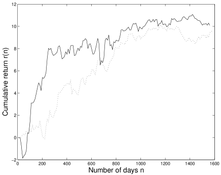
Figure 3: Cumulative return of the market neutral algorithm applied to daily price data of the Dow Jones stock index (dotted line), as well as the CAC40 stock index (solid line) over the period 3/01/2000-2/5/2006. First half of the time period for the Dow Jones index was used in sample to determine the best choice among three values of the parameter $m=5,10,15$ days. Second half of the time period for the Dow Jones index as well as full period of the CAC40 index was done out of sample with $m=10$. As a measure of the performance of the algorithm, the Sharpe ratio was found to be 2.0 and 2.94 for the Dow Jones, respectively CAC40 price time series. A trading cost of 0.1% was included for each transaction.

The algorithm was then applied to real market data. However as noted in Gil a general problem arises because of long term drifts in anchor of the price, $\bar{A_{i}}$, which is never truely “quasi-static”. I.e. $\bar{A_{i}}$ is time dependent, and for sufficient strong drifts the return of the algorithm was then shown to vanish. In order to circumvent this obstacle the algorithm was modified so as always to be market neutral independent of any drift the portfolio of the $N$ assets might perform. Figure 3 shows the market neutral algorithm applied to real market data of the Dow Jones stock index, as well as the CAC40 stock index. First half of the time period for the Dow Jones index was used in sample to determine the best choice among three values of the parameter $m=5,10,15$ days. Only three possible values corresponding to one, two or three weeks were probed in sample. Since the present paper look into any possible impact coming from human anchoring, using only daily or weekly data seems a priori justified since the higher the frequency of the trading (say seconds/minutes) the more computer dominated becomes the trading. In order to look for arbitrage possibilities weekly data was used so as to avoid impact of transaction costs by trading too often. Another reason only to have looked at weekly data is because of the main claim put forward in this paper where market participants by actively following the price thereby create a subjective reference (anchor) and memory of when an asset is “cheap” or “expensive”. Several studies on the persistence of human memory have reported sleep as well as post-training wakefulness before sleep, to play an important role in the offline processing and consolidation of memoryPeigneux . It therefore makes sense to think that conscious as well as unconscious mental processes influence the judgements of people who specializes in active trading on a day-to-day basis. The out of sample profit from the market neutral trading algorithm (with transaction costs taking into account) on the CAC40 index as well as the second period performance on the Dow Jones index, gives evidence that anchoring does indeed play a dominant role on the weekly price fixing of the Dow Jones and CAC40 stock markets, and reconfirms the claim in Gil where especially the policy imposed by the European Monetary System was shown to lead to arbitrage possibilities. The results also gives yet another illustration on the difficulty proving market efficiency by only considering lower order correlations in past price time series.

In conclusion a trading algorithm inspired by biological motors and introduced by L. Gil, is suggested as a testing ground for anchoring in financial markets. An exact solution of the algorithm was found for arbitrary price distributions and the algorithm was extended to cover the case of a market neutral portfolio. The exposure of arbitrage possibilities by the market neutral algorithm reveals additional evidence that anchoring is indeed involved in the decision making of market participants.

The author is grateful to L. Gil for valuable discussions.

References

- (1) L. Gil, arXiv:0705.2097 2007
- (2) A. Tversky and D. Kahneman, Science 185, 1124 (1974).
- (3) G. Ye, SSRN-id548862, (2004).
- (4) A. Dodonova and Y. Khoroshilov, Applied Economics Letters 11, 307 (2004).
- (5) G. B. Northcraft and M. A. Neale, Organizational Behavior and Human Decision Processes, 39, 84 (1987).
- (6) P. Bofinger and R. Schmidt, Discussion Paper Series - Centre For Economic Policy Research London, ISSU 4235 (2004).
- (7) H. M. Shefrin and M. Statman Journal of Finance 40, 777 (1985).
- (8) K. Heilmann, V. Laeger and A. Oehler, Proceedings of the 25th Annual Colloquium, IAREP, Wien (2000).
- (9) M. Weber and C. F. Camerer, Journal of Economic Behavior & Organization 33, 167 (1998).
- (10) J. V. Andersen and D. Sornette, Europhys. Lett. 70, 697 (2005).
- (11) D. Sornette and J. V. Andersen, Int. J. Mod. Phys. C11, 713 (2000).
- (12) P. Peigneux, P. Orban, E. Balteau, C. Degueldre and A. Luxen, PLoS Biology, Vol. 4, No.4, e100 doi:10.1371/journal.pbio.0040100 (2006).