Orbital order in degenerate Hubbard models : A variational study

Abstract

We use the Gutzwiller variational many-body theory to investigate the stability of orbitally ordered states in a two-band Hubbard-model without spin degrees of freedom. Our results differ significantly from earlier Hartree-Fock calculations for this model. The Hartree-Fock phase diagram displays a large variety of orbital orders. In contrast, in the Gutzwiller approach orbital order only appears for densities in a narrow region around half filling.

1 Introduction

The investigation of orbital degrees of freedom has become an important field in theoretical solid-state physics over the past two decades. There are a number of materials which are believed to show phase transitions with orbital order parameters. Among them, the perovskite manganites, e.g., ${\rm La}_{1-x}{\rm Sr}_{x}{\rm MnO}_{3}$, have attracted particular interest because of the colossal magnetoresistance behaviour which is observed in these materials. In theoretical studies on manganites, one often neglects the almost localised Mn $t_{2{\rm g}}$ orbitals and investigates solely the electronic properties of a systems with two $e_{\rm g}$ orbitals per lattice site. In order to study the ferromagnetic phase of such a model, Takahashi and Shiba [1] further neglected the spin-degrees of freedom because the Hund’s rule coupling is assumed to align the spins in the two $e_{\rm g}$ orbitals.

The mean-field study in [1] found a surprisingly large number of stable orbitally ordered phases for the spinless $e_{\rm g}$ model. However, it is well known that mean-field approximations tend to overestimate the stability of ordered phases in correlated electron systems. Therefore, the purpose of this work is to reinvestigate the two-orbital Hubbard model without spin-degrees of freedom by means of the Gutzwiller variational many-body theory.

Our paper is organised as follows: The Hamiltonian and the different types of order parameters that we are going to investigate are discussed in section 2. In section 3 we introduce Gutzwiller wave functions and derive an approximate expression for the variational ground-state energy. Numerical results are presented in section 4 and a brief summary closes our presentation in section 5.

2 Model system and types of order parameters

We investigate a two-orbital ($e_{\rm g}$-type) Hubbard model [2] without spin-degrees of freedom,

$$\hat{H} = \hat{H}_{0}+\hat{H}_{U}\,,$$ (1)

$$\hat{H}_{0} \equiv \sum_{i,j}\sum^{2}_{b,b^{\prime}=1}t^{b,b^{\prime}}_{i,j}\hat{c}^{\dagger}_{i,b}\hat{c}_{j,b^{\prime}}\,,$$ (2)

$$\hat{H}_{U} \equiv U\sum_{i}\hat{n}_{i,1}\hat{n}_{i,2}\,.$$ (3)

Here, the tight-binding parameters $t^{b,b^{\prime}}_{i,j}$ describe hopping processes between orbitals $b,b^{\prime}$ on cubic lattice sites ${\bf R}_{i}$ and ${\bf R}_{j}$, respectively. The Hamiltonian (1) is formally equivalent to the standard one-band Hubbard model if the indices $b,b^{\prime}$ are regarded as spins. However, the tight-binding parameters in (2) would be unusual for a genuine one band model since they contain inter-orbital hopping-terms. The Hubbard parameter $U$ in (3) is derived from $U=U^{\prime}-J$ where $U^{\prime}$ and $J$ are the Coulomb and the exchange interaction between electrons in different $e_{\rm g}$ orbitals.

We restrict our investigation to systems with only nearest neighbour hopping since additional hopping terms would only destabilise the orbital order we are interested in. For $e_{\rm g}$ orbitals $|z_{1}\rangle\equiv|x^{2}-y^{2}\rangle$, $|z_{2}\rangle\equiv|3z^{2}-r^{2}\rangle$ and hopping parameters $t_{dd\sigma}=1{\rm eV}$, $t_{dd\delta}=0{\rm eV}$ [3], the one-particle Hamiltonian in momentum space reads

$$\hat{H}_{0}=\sum_{{\bf k}}\sum_{b,b^{\prime}}\epsilon^{b,b^{\prime}}_{z;{\bf k}}\hat{c}^{\dagger}_{z;{\bf k},b}\hat{c}_{z;{\bf k},b^{\prime}}\,,$$ (4)

with [3]

$$\epsilon^{1,1}_{z;{\bf k}} = (\cos{(k_{x})}+\cos{(k_{y})}+4\cos{(k_{z})})/2\,,$$

$$\epsilon^{2,2}_{z;{\bf k}} = 3(\cos{(k_{x})}+\cos{(k_{y})})/2\,,$$ (5)

$$\epsilon^{1,2}_{z;{\bf k}} = -\sqrt{3}(\cos{(k_{x})}-\cos{(k_{y})})/2=\epsilon^{2,1}_{z;{\bf k}}\,.$$

The ${\bf k}$-integrated density of states $D(\varepsilon)$ that results from this band structure is shown in figure 1.

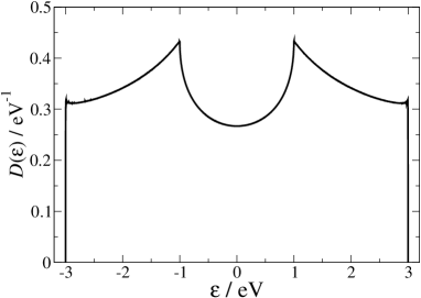
Figure 1: Density of states of the model system (4) .

For our investigation of orbital order we need to introduce two more basis representations of the orbital space,

$$|x_{1}\rangle \equiv \frac{1}{\sqrt{2}}(|z_{1}\rangle+|z_{2}\rangle)\,,$$ (6)

$$|x_{2}\rangle \equiv \frac{1}{\sqrt{2}}(|z_{1}\rangle-|z_{2}\rangle)\,,$$

and

$$|y_{1}\rangle \equiv \frac{1}{\sqrt{2}}(|z_{1}\rangle+\rm{i}|z_{2}\rangle)\,,$$ (7)

$$|y_{2}\rangle \equiv \frac{1}{\sqrt{2}}(|z_{1}\rangle-\rm{i}|z_{2}\rangle)\,.$$

The dispersion relations in momentum space for the ‘$x$’- and the ‘$y$’-basis become

$$\epsilon^{1,1}_{x;{\bf k}} = ((2-\sqrt{3})\cos{(k_{x})}+(2+\sqrt{3})\cos{(k_{y})}+2\cos{(k_{z})})/2\,,$$ (8)

$$\epsilon^{2,2}_{x;{\bf k}} = ((2+\sqrt{3})\cos{(k_{x})}+(2-\sqrt{3})\cos{(k_{y})}+2\cos{(k_{z})})/2,$$

$$\epsilon^{1,2}_{x;{\bf k}} = \cos{(k_{x})}+\cos{(k_{y})}-2\cos{(k_{z})})/2=\epsilon^{2,1}_{x;{\bf k}}\,,$$

$$\epsilon^{1,1}_{y;{\bf k}} = \cos{(k_{x})}+\cos{(k_{y})}+\cos{(k_{z})}=\epsilon^{2,2}_{y;{\bf k}}\,,$$ (9)

$$\epsilon^{1,2}_{y;{\bf k}} = ((1+\sqrt{3}\rm{i})\cos{(k_{x})}+(1-\sqrt{3}\rm{i})\cos{(k_{y})}-2\cos{(k_{z})})/2\,,$$

$$\epsilon^{2,1}_{y;{\bf k}} = \left(\epsilon^{1,2}_{y;{\bf k}}\right)^{*}\,.$$

The interaction term (3) has the same form for all three basis representations $\xi=x,y,z$.

We describe orbital order in our model system (1) through the parameters

$$\tau_{\xi;i} \equiv (\langle\hat{n}_{i,\xi_{1}}\rangle-\langle\hat{n}_{i,\xi_{2}}\rangle)/2\,,$$ (10)

$$\hat{n}_{i,\xi_{b}} \equiv \hat{c}^{\dagger}_{i,\xi_{b}}\hat{c}_{i,\xi_{b}}\,,$$ (11)

for each of the three representations $\xi$. By using the Pauli matrices $\tilde{1},\tilde{\tau}^{x},\tilde{\tau}^{y},\tilde{\tau}^{z}$ the order parameter can also be written as (compare reference [1])

$$\tau_{\xi;i}=\frac{1}{2}\sum_{b,b^{\prime}}\langle\hat{c}^{\dagger}_{i,z_{b}}(\tilde{\tau}^{\xi})_{b,b^{\prime}}\hat{c}_{i,z_{b^{\prime}}}\rangle\,.$$ (12)

Besides the orbital character of the order-parameter we need to specify its lattice site dependence. Following reference [1] we consider orders of the form

$$\tau_{\xi;i}=\tau_{\xi,0}\exp{({\rm i}{\bf Q}{\bf R}_{i})}$$ (13)

with commensurate vectors ${\bf Q}$ which belong to the $\Gamma$ point (${\bf Q}=(0,0,0)$), the $R$ point (${\bf Q}=(\pi,\pi,\pi)$), the $X$ point (${\bf Q}=(0,0,\pi)$), and the $M$ point (${\bf Q}=(\pi,\pi,0)$). The real parameter $\tau_{\xi,0}$ in (13) is independent of the lattice site vector ${\bf R}_{i}$ and assumed to be positive. Note, that for vectors ${\bf Q}\neq(0,0,0)$ equation (13) divides the lattice into an ‘$A$’-lattice with a majority $\xi_{1}$ occupation ($\tau_{\xi;i}>0$), and a ‘$B$’-lattice with a majority $\xi_{2}$ occupation ($\tau_{\xi;i}<0$).

3 Gutzwiller wave-functions

3.1 Definitions

For an investigation of the Hamiltonian (1) we use Gutzwiller variational wave functions [4] which are defined as

$$|\Psi_{\rm G}\rangle\equiv\prod_{i}\hat{P}_{i}|\Psi_{0}\rangle\;.$$ (14)

Here, $|\Psi_{0}\rangle$ is a normalised quasi-particle vacuum and the local correlator has the form

$$\hat{P}_{i}=\sum_{I}\lambda_{i,I}\hat{m}_{i,I}$$ (15)

where $\hat{m}_{I}=|I\rangle\langle I|$ projects onto the four local configuration states $|I\rangle$, i.e., the empty state $|\emptyset\rangle$, the doubly occupied state $|d\rangle$ and the two single electron states $|\xi_{1}\rangle,|\xi_{2}\rangle$. Note, that $|\xi_{1}\rangle$ and $|\xi_{2}\rangle$ depend on the orbital representation $\xi$ whereas the states $|\emptyset\rangle$ and $|d\rangle$ are invariant under the orbital transformations (6) and (7). For the variational parameters $\lambda_{i,I}$ we make an Ansatz which is consistent with the spatial symmetry of the order parameter,

$$\lambda_{i,\emptyset} = \lambda_{\emptyset}\,,$$ (16)

$$\lambda_{i,d} = \lambda_{d}\,,$$ (17)

$$\lambda_{i,\xi_{1}} = \lambda_{s}+\delta\lambda_{s}\exp{({\rm i}{\bf Q}{\bf R}_{i})}\,,$$ (18)

$$\lambda_{i,\xi_{2}} = \lambda_{s}-\delta\lambda_{s}\exp{({\rm i}{\bf Q}{\bf R}_{i})}\,,$$ (19)

where the parameters $\lambda_{\emptyset}$,$\lambda_{d}$, $\lambda_{s}$,$\delta\lambda_{s}$ are independent of the lattice site vector ${\bf R}_{i}$.

A more general ansatz for the Gutzwiller correlator $\hat{P}$ which also includes non-diagonal configuration transfer operators $|I\rangle\langle I^{\prime}|$ has been studied in reference [5]. As we will see below (section 3.2), it is sufficient for our calculations in this work to consider only diagonal operators in $\hat{P}_{i}$.

3.2 Evaluation in infinite dimensions

For any practical use of a variational wave-function it is essential that the expectation value of the Hamilton can be calculated. However, despite the simplicity of the Gutzwiller wave-function the evaluation of

$$E_{\rm var}=\langle\hat{H}\rangle_{\Psi_{\rm G}}$$ (20)

poses a difficult many-particle problem that cannot be solved in general. Gutzwiller introduced an approximate evaluation scheme that was based on quasi-classical counting arguments. More recent derivations of this approximation can be found in references [6, 7]. Analytically exact evaluations were later found to be possible in one dimension [8, 9, 10], and in infinite spatial dimension [11]. The results of the latter evaluation turned out to be equivalent to the Gutzwiller approximation for systems which can be studied within this approach. The evaluation scheme in infinite dimensions was later generalised for the investigation of multi-band Hubbard models [12] and superconducting systems [5, 13]. We will use these exact results in infinite dimensions as an approximation in order to evaluate expectation values of our Hamiltonian (1).

We only consider single-particle wave functions $|\Psi_{0}\rangle$ in (14) for which the local density matrix $\tilde{C}^{0}$ with the matrix elements

$$C^{0}_{i,\xi_{b},\xi_{b^{\prime}}}\equiv\langle\hat{c}^{\dagger}_{i,\xi_{b}}\hat{c}_{i,\xi_{b^{\prime}}}\rangle_{\Psi_{0}}\equiv n^{0}_{i,\xi_{b}}\delta_{b,b^{\prime}}$$ (21)

is diagonal with respect to $b,b^{\prime}$. Finite non-diagonal elements in $\tilde{C}^{0}$ could only appear if we were mixing different order parameters.

As shown in [5] the four parameters $\lambda_{i,I}$ for a lattice site $i$ have to obey the constraints

$$1 = \langle\hat{P}_{i}^{2}\rangle_{\Psi_{0}}\;,$$ (22)

$$C^{0}_{i,\xi_{b},\xi_{b^{\prime}}} = \langle\hat{P}^{2}_{i}\hat{c}^{\dagger}_{i,\xi_{b}}\hat{c}_{i,\xi_{b^{\prime}}}\rangle_{\Psi_{0}}\;.$$ (23)

Our correlation operator (15) automatically fulfils the constraints (23) for $b\neq b^{\prime}$. This is the reason why it was allowed in the first place to include only diagonal operators $\hat{m}_{i,I}$ in (15). Consequently, instead of (23) we only need to consider the diagonal constraints

$$n^{0}_{i,\xi_{b}}=\langle\hat{P}^{2}_{i}\hat{n}_{i,\xi_{b}}\rangle_{\Psi_{0}}\;.$$ (24)

All constraints can be solved explicitly if we use the results for local expectation values

$$m_{i,I}\equiv\langle\hat{m}_{i,I}\rangle_{\Psi_{\rm G}}=\lambda_{i,I}^{2}\langle\hat{m}_{i,I}\rangle_{\Psi_{0}}$$ (25)

which hold in infinite spatial dimensions. With (25) we can use the expectation values $m_{i,I}$ as new variational parameters instead of $\lambda_{i,I}$. The constraints then read

$$1 = m_{i,\emptyset}+m_{i,d}+m_{i,\xi_{1}}+m_{i,\xi_{2}}\,,$$ (26)

$$n^{0}_{i,\xi_{b}} = m_{i,\xi_{b}}+m_{i,d}\,.$$ (27)

and can be readily solved by expressing all local occupancies in terms of the average numbers of doubly occupied sites $m_{i,d}$,

$$m_{i,\emptyset} = 1-n^{0}_{i,\xi_{1}}-n^{0}_{i,\xi_{2}}+m_{i,d}\,,$$ (28)

$$m_{i,\xi_{b}} = n^{0}_{i,\xi_{b}}-m_{i,d}\,.$$ (29)

Apart from the still unspecified one particle wave function $|\Psi_{0}\rangle$ and the corresponding local density matrices $\tilde{C}^{0}_{i}$ the probabilities $m_{i,d}$ are the only remaining variational parameters. Note, that (29) leads to

$$n_{i,\xi_{b}}\equiv\langle\hat{n}_{i,\xi_{b}}\rangle_{\Psi_{\rm G}}=n^{0}_{i,\xi_{b}}$$ (30)

for the orbital densities in the correlated Gutzwiller wave-function. We skip the explicit declaration of the orbital representation $\xi$ for the rest of this chapter and write $b$ instead of $\xi_{b}$ in all indices.

In infinite dimensions the expectation value of the one particle Hamiltonian (2) becomes [12]

$$E_{0}=\langle\hat{H}_{0}\rangle_{\Psi_{\rm G}} = \sum_{i,j}\sum_{b,b^{\prime}}\sqrt{q_{i,b}q_{j,b^{\prime}}}t^{b,b^{\prime}}_{i,j}\langle\hat{c}^{\dagger}_{i,b}\hat{c}_{j,b^{\prime}}\rangle_{\Psi_{0}}\equiv\langle\hat{H}^{\prime}_{0}\rangle_{\Psi_{0}}$$ (31)

where we introduced the well known Gutzwiller loss factors [4]

$$q_{i,b}=\frac{1}{n^{0}_{i,b}(1-n^{0}_{i,b})}\left(\sqrt{m_{i,\emptyset}m_{i,b}}+\sqrt{m_{i,\bar{b}}m_{i,d}}\right)^{2}$$ (32)

and $\bar{b}$ is defined via $\bar{1}\equiv 2$ and $\bar{2}\equiv 1$.

The lattice symmetry of the order parameter leads to further simplifications. We introduce the majority and the minority orbital density

$$n^{0}_{\pm}\equiv n^{0}\pm\tau_{0}$$ (33)

such that

$$n^{0}_{i,1}=n^{0}_{\pm}\,\,,\,\,n^{0}_{i,2}=n^{0}_{\mp}\,.$$ (34)

The upper and lower signs in (34), and in corresponding equations below, belong to lattice sites $i\in A$ and $i\in B$, respectively. For the other local expectation values we find

$$m_{i,d} = m_{d}\,,$$ (35)

$$m_{i,1} \equiv m_{\pm}=n^{0}_{\pm}-m_{d}\,,$$ (36)

$$m_{i,2} \equiv m_{\mp}=n^{0}_{\mp}-m_{d}\,,$$ (37)

$$m_{i,\emptyset} = 1-2n^{0}+m_{d}\,.$$ (38)

A similar notation is introduced for the $q$-factors

$$q_{i,1}\equiv q_{\pm}\,\,\,\,,\,\,\,q_{i,2}\equiv q_{\mp}$$ (39)

where

$$q_{\pm}\equiv\frac{1}{n^{0}_{\pm}(1-n^{0}_{\pm})}\left(\sqrt{m_{\emptyset}m_{\pm}}+\sqrt{m_{\mp}m_{d}}\right)^{2}\;.$$ (40)

The expectation value (31) splits into four components

$$E_{0}=q_{+}E^{++}+q_{-}E^{--}+\sqrt{q_{+}q_{-}}(E^{+-}+E^{-+})$$ (41)

which belong to the four different hopping channels between majority (‘$+$’) and minority (‘$-$’) states. In momentum space, the one-particle expectation values in (41) can be written as

$$E^{\omega\omega^{\prime}} = \frac{1}{4}\sum_{{\bf k}}\sum_{b,b^{\prime}}\epsilon_{k}^{bb^{\prime}}\left(M^{1}_{b,b^{\prime}}\langle\hat{c}^{\dagger}_{{\bf k},b}\hat{c}_{{\bf k},b^{\prime}}\rangle_{\Psi_{0}}+\omega M^{2}_{b,b^{\prime}}\langle\hat{c}^{\dagger}_{{\bf k}+{\bf Q},b}\hat{c}_{{\bf k},b^{\prime}}\rangle_{\Psi_{0}}\right.$$

$$\left.+\omega^{\prime}M^{3}_{b,b^{\prime}}\langle\hat{c}^{\dagger}_{{\bf k},b}\hat{c}_{{\bf k}+{\bf Q},b^{\prime}}\rangle_{\Psi_{0}}+\omega\omega^{\prime}M^{4}_{b,b^{\prime}}\langle\hat{c}^{\dagger}_{{\bf k}+{\bf Q},b}\hat{c}_{{\bf k}+{\bf Q},b^{\prime}}\rangle_{\Psi_{0}}\right)$$

where $\omega,\omega^{\prime}$ represent the $+$ or $-$ signs and the coefficients $M^{\gamma}_{b,b^{\prime}}$ are given as the elements of the matrices

$$\tilde{M}^{1} = \left(\begin{array}[]{cc}1&1\\ 1&1\end{array}\right)\;\;\;\;\;,\;\;\;\tilde{M}^{2}=\left(\begin{array}[]{cc}1&1\\ -1&-1\end{array}\right)\;,$$ (47)

$$\tilde{M}^{3} = \left(\begin{array}[]{cc}1&-1\\ 1&-1\end{array}\right)\;\;\;,\;\;\tilde{M}^{4}=\left(\begin{array}[]{cc}1&-1\\ -1&1\end{array}\right)\;.$$ (52)

For the evaluation of the expectation values in (3.2) we need to determine the one-particle wave function $|\Psi_{0}\rangle$. Following reference [5, 14], $|\Psi_{0}\rangle$ is given as the ground state of the effective one-particle Hamiltonian

$$\hat{H}_{0}^{\rm eff}=\hat{H}^{\prime}_{0}-\eta\sum_{i}\exp{({\rm i}{\bf Q}{\bf R}_{i})}(\hat{n}_{i,1}-\hat{n}_{i,2})\,,$$ (53)

where $\hat{H}^{\prime}_{0}$ was introduced in (31) and the term proportional to the variational parameter $\eta$ allows to vary the order parameter $\tau_{0}$.

In this work, we only aim to investigate the stability of the orbitally unordered state. Therefore we just need to analyse the energy expression (41) for small values of the order parameter $\tau_{0}$. An expansion of the $q$-factors (40) up to second order in $\tau_{0}$,

$$q_{\pm}\approx\tilde{q}_{0}\pm\tilde{q}_{1}\tau_{0}+\tilde{q}_{2}\tau_{0}^{2}\,$$ (54)

yields

$$\sqrt{q_{+}q_{-}}\approx\tilde{q}_{0}+\left(\tilde{q}_{2}-\frac{\tilde{q}^{2}_{1}}{2\tilde{q}_{0}}\right)\tau_{0}^{2}\,.$$ (55)

Note, that the coefficients $\tilde{q}_{\gamma}$ are still functions of $n^{0}$ and $m_{d}$. To leading order in $\tau_{0}$ the effective Hamiltonian (53) becomes

$$\hat{H}_{0}^{\rm eff}=\tilde{q}_{0}\sum_{{\bf k}}\sum_{b,b^{\prime}}\epsilon^{b,b^{\prime}}_{{\bf k}}\hat{c}^{\dagger}_{{\bf k},b}\hat{c}_{{\bf k},b^{\prime}}-\eta\sum_{{\bf k}}\left(\hat{c}^{\dagger}_{{\bf k},1}\hat{c}_{{\bf k}+{\bf Q},1}-\hat{c}^{\dagger}_{{\bf k},2}\hat{c}_{{\bf k}+{\bf Q},2}\right)$$ (56)

since we can set $q_{i,b}=\tilde{q}_{0}$ in $\hat{H}^{\prime}_{0}$, eq. (31). The one-particle Hamiltonian (56) is easily diagonalised numerically. This diagonalisation yields the coefficients in the quadratic expansion of (3.2)

$$E^{\pm\pm} = E_{0}+E_{2}\tau_{0}^{2}\,,$$ (57)

$$E^{\pm\mp} = E^{\prime}_{0}+E^{\prime}_{2}\tau_{0}^{2}\,,$$ (58)

and, consequently, of the variational ground state energy

$$E_{\rm var}=\tilde{q}_{0}E_{0}^{\rm tot}+\left(\tilde{q}_{0}E_{2}^{\rm tot}+\tilde{q}_{2}E_{0}^{\rm tot}-E^{\prime}_{0}\frac{\tilde{q}^{2}_{1}}{\tilde{q}_{0}}\right)\tau_{0}^{2}+Um_{d}\,.$$ (59)

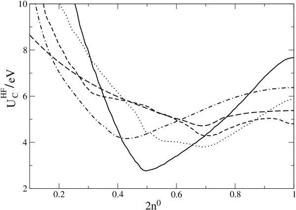
Figure 2: Critical interaction strength in Hartree Fock-theory for the orders $\tau^{y}_{R}$ (straight), $\tau^{z}_{M}$ (dashed), $\tau^{z(x)}_{\Gamma}$ (long-dashed), $\tau^{y}_{M}$ (dotted), and $\tau^{x}_{X}$ (dash-dotted). These phases are not stable within the Gutzwiller theory.

Here, we introduced

$$E_{\gamma}^{\rm tot} \equiv 2(E_{\gamma}+E^{\prime}_{\gamma})$$ (60)

for $\gamma=0$ or $2$. The minimisation of $E_{var}$ with respect to $m_{d}$ can be carried out for $\tau_{0}=0$

$$E_{0}^{\rm tot}\left.\frac{\partial\tilde{q}_{0}}{\partial m_{d}}\right|_{m_{d}=\bar{m}_{d}}+U=0$$ (61)

and determines the optimum number $\bar{m}_{d}$ of doubly occupied sites as a function of $U$ and $n^{0}$. This allows the expansion of the variational energy purely in terms of $\tau_{0}$

$$E_{\rm var}=\tilde{q}_{0}E_{0}^{\rm tot}+c_{\tau_{0}}\tau_{0}^{2}\,.$$ (62)

A negative sign of the coefficient

$$c_{\tau_{0}}=\tilde{q}_{0}E_{2}^{\rm tot}+\tilde{q}_{2}E_{0}^{\rm tot}-E^{\prime}_{0}\frac{\tilde{q}^{2}_{1}}{\tilde{q}_{0}}=c_{\tau_{0}}(U,n^{0})$$ (63)

in (62) indicates the instability of the unordered state. Note that a positive $c_{\tau_{0}}$ not necessarily proves the stability of the unordered state since it does not exclude first order transitions.

In Hartree-Fock theory a quadratic expansion of the ground-state energy leads to

$$E_{\rm var}^{\rm HF}=E_{0}^{\rm tot}+(E_{2}^{\rm tot}-U)\tau_{0}^{2}\,,$$ (64)

and the critical interaction strength in this approach is therefore given as

$$U^{\rm HF}_{\rm C}=E_{2}^{\rm tot}\,.$$ (65)

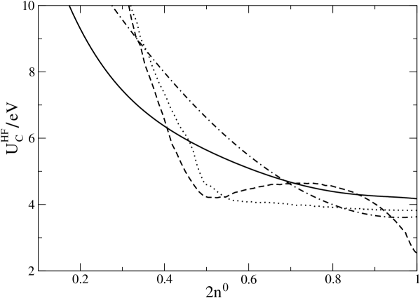
Figure 3: Critical interaction strength in Hartree Fock-theory for the orders $\tau^{y}_{\Gamma(X)}$ (straight), $\tau^{z(x)}_{R}$ (dashed), $\tau^{x}_{M}$ (dotted), and $\tau^{z}_{X}$ (dash-dotted).

4 Results

In figures 2 and 3 we show the critical interaction strength (65) in Hartree-Fock theory as a function of density for the various types of orbital order introduced in section 2. Our data agree very well with those reported in reference [1]. Note that in Hartree-Fock theory the critical interaction strength is finite for all densities $n^{0}>0$ and diverges only in the limit $n^{0}\rightarrow 0$.

The phases in figure 2 are not stable within our correlated Gutzwiller approach for all densities and interaction parameters. This holds in particular for the order parameter $\tau_{R}^{y}$ which has surprisingly small critical values $U^{\rm HF}_{\rm C}$ around quarter filling $2n^{0}\approx 0.5$.

For the four surviving phases (figure 3) we show the ratio $U^{\rm GW}_{\rm C}/U^{\rm HF}_{\rm C}$ of the critical parameters in Gutzwiller and Hartree-Fock theory as a function of density in figure 4.

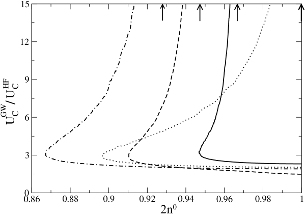
Figure 4: Critical interaction strength in Gutzwiller-theory for the orders $\tau^{y}_{\Gamma(X)}$ (straight), $\tau^{z(x)}_{R}$ (dashed), $\tau^{x}_{M}$ (dotted), and $\tau^{z}_{X}$ (dash-dotted). The arrows indicate the critical densities $2n_{\rm c}^{0}$ for $U\rightarrow\infty$.

Apparently, there is only a narrow window of densities around half filling $2n^{0}\approx 1$ where orbital order occurs in the Gutzwiller theory. This is in stark contrast to the Hartree-Fock findings in figure 3. For three of the phases the orbital order may disappear again if $U$ exceeds some second critical value $\tilde{U}^{\rm GW}_{\rm C}>U^{\rm GW}_{\rm C}$. This behaviour is also different from the Hartree-Fock theory in which the orbital order is stable for all $U>U^{\rm HF}_{\rm C}$. Mathematically, the appearance of the second critical parameter $\tilde{U}^{\rm GW}_{\rm C}$ is due to the fact that $\tilde{q}_{2}$ in (54) has a minimum as a function of $m_{d}$. Hence, the coefficient $c_{\tau_{0}}$ may have one or two roots as a function of $U$, depending on the other parameters in (63). The appearance of the second transition is therefore a genuine many-particle effect. Only one of the four orders, $\tau^{x}_{M}$, is unstable in the limit $U\rightarrow\infty$ for all densities. For the three other orders we find critical densities $n_{\rm c}^{0}$ with a stable order for all $n^{0}>n_{\rm c}^{0}$ in the limit $U\rightarrow\infty$. The values of $n_{\rm c}^{0}$ are displayed by arrows in figure 4.

The failure of Hartree-Fock theory to describe the orbitally ordered phases of the two-band model is not surprising. It is well known, for example, that Hartree-Fock theory also grossly overestimates the stability of ferromagnetic ground states in the one-band Hubbard model [15]. Ferromagnetism in this model requires very peculiar densities of states or very large local Coulomb interactions [16]. The simple Stoner criterium of the Hartree-Fock theory, however, predicts ferromagnetism for all densities and for small Coulomb interactions.

Orbital order in the two-band model at infinite $U$ has also been investigated in reference [17]. In their work the authors report a complete disappearance of all types of orbital order seen in the Hartree-Fock theory.

5 Summary

We have reported results for orbital order in a two-orbital Hubbard-model without spin-degrees of freedom. In a previous work which was based on Hartree-Fock calculations, this system seemed to exhibit a surprisingly large variety of orbitally-ordered phases. In our study in this work we have employed the Gutzwiller variational theory which is known to be more reliable than the Hartree-Fock theory for systems with medium to strong local Coulomb interaction. Most of the phases found in the Hartree-Fock approach turned out to be unstable in the Gutzwiller-theory. Orbital order only appears for densities near half filling in our calculation. Unlike in Hartree-Fock theory, it may happen that an orbitally ordered phase which is stable for correlation parameters $U>U^{\rm GW}_{\rm C}$ becomes unstable again if $U$ exceeds a second critical value $\tilde{U}^{\rm GW}_{\rm C}>U^{\rm GW}_{\rm C}$. This second transition is a genuine many-particle effect.

Our findings show that the stability of phases with broken symmetry for correlated electron systems can be grossly overestimated by the Hartree-Fock mean-field theory. It is quite likely that similar problems appear in LDA+U calculations where the local Coulomb interaction is also treated on a Hartree-Fock level.

References

References

• [1] Takahashi A and Shiba H 2000 J. Phys. Soc. Jpn. 69 3328
• [2] Hubbard J 1963 Proc. R. Soc. A 276 238
• [3] Slater J C and Koster G F 1954 Phys. Rev. 94 1498
• [4] Gutzwiller M C 1963 Phys. Rev. Lett. 10 159
• [5] Bünemann J, Gebhard F, and Weber W 2005 Frontiers in Magnetic Materials, ed A Narlikar (Berlin: Springer)
• [6] Vollhardt D 1984 Rev. Mod. Phys. 56 99
• [7] Bünemann J 1998 Eur. Phys. J. B 4 29
• [8] Metzner W and Vollhardt D 1987 Phys. Rev. Lett. 59121
• [9] Metzner W and Vollhardt D 1988 Phys. Rev. B 37 7382
• [10] Kollar M and Vollhardt D 2002 Phys. Rev. B 65 155121
• [11] Gebhard F 1990 Phys. Rev. B 41 9452
• [12] Bünemann J, Weber W, and Gebhard F 1998 Phys. Rev. B 57 6896
• [13] Bünemann J, Gebhard F, Radnóczi K, and Fazekas K 2005 J. Phys. Cond. Matt. 17 3807
• [14] Bünemann J, Gebhard F, and Thul R 2003 Phys. Rev B 67 75103
• [15] Fazekas P 1999 Lecture Notes on Electron Correlation and Magnetism (Singapore: World Scientific)
• [16] Ulmke M 1998 Eur. Phys. J. B 1 301
• [17] Feiner L F and Oles A M 2005 Phys. Rev. B 71 144422