Shear-Induced Chaos

Abstract

Guided by a geometric understanding developed in earlier works of Wang and Young, we carry out some numerical studies of shear-induced chaos. The settings considered include periodic kicking of limit cycles, random kicks at Poisson times, and continuous-time driving by white noise. The forcing of a quasi-periodic model describing two coupled oscillators is also investigated. In all cases, positive Lyapunov exponents are found in suitable parameter ranges when the forcing is suitably directed.

Introduction

This paper presents a series of numerical studies which investigate the use of shear in the production of chaos. The phenomenon in question can be described roughly as follows: An external force is applied to a system with tame, nonchaotic dynamics. If the forcing is strategically applied to interact with the shearing in the underlying dynamics, it can sometimes lead to the folding of phase space, which can in turn lead to positive Lyapunov exponents for a large set of initial conditions. This phenomenon, which we call shear-induced chaos, occurs in a wide variety of settings, including periodically-forced oscillators. For a topic as general as this, it is difficult to compile a reasonable set of references. We have not attempted to do that, but mention that the first known observation of a form of this phenomenon was by van der Pol and van der Mark 80 years ago [21]. Other references related to our work will be mentioned as we go along.

The starting point of the present work is a series of papers by Wang and Young [22, 23, 24, 25]. In these papers, the authors devised a method for proving the existence of strange attractors and applied their techniques to some natural settings; two of their main examples are periodically-kicked oscillators and systems undergoing Hopf bifurcations. They identified a simple geometric mechanism to explain how the chaotic behavior comes about. Because of the perturbative nature of their analysis, however, the kicks in these results have to be followed by very long periods of relaxation. In other words, the chaos in these attractors develop on a very slow time scale. Relevant parts of the results of Wang and Young are reviewed in Sect. 1.

The aim of the present paper is to study shear-induced chaos in situations not accessible by current analytic tools. We believe that this phenomenon is widespread, meaning it occurs for large sets of parameters, and that it is robust, meaning it does not depend sensitively on the type of forcing or even background dynamics as long as certain geometric conditions are met. We validate these ideas through a series of numerical studies in which suitable parameters are systematically identified following ideas from [23] and [24]. Four separate studies are described in Sects. 2– 5. The first three studies involve an oscillator driven by different types of forcing (both deterministic and stochastic); in these studies, the unforced system is a simple linear shear flow model. In the fourth study, the unforced dynamics are that of a coupled oscillator system described by a (periodic or quasi-periodic) flow on the $2$-torus.

The linear shear flow used in Studies 1–3 has been studied independently in [27] and [23]. It is the simplest system known to us that captures all the essential features of typical oscillator models relevant to shear-induced chaos. Moreover, these features appear in the system in a way that is easy to control, and the effects of varying each are easy to separate. This facilitates the interpretation of our theoretical findings in more general settings in spite of the fact that numerical studies necessarily involve specific models.

We mention that our results on shear flows are potentially applicable to a setting not discussed here, namely that of the advection and mixing of passive scalar tracers in (weakly compressible) flows.

Finally, we remark that this work exploits the interplay between deterministic and stochastic dynamics in the following way: The geometry in deterministic models are generally more clear-cut. It enables us to extract more readily the relationship between quantities and to deduce the type of results these relationships may lead. Results for stochastic models, on the other hand, tend to be more provable than their counterparts in deterministic models, where competing scenarios lead to very delicate dependences on parameters. Our numerical results on stochastic forcing in Studies 2–4 point clearly to the possibility of (rigorous) theorems, some versions of which, we hope, will be proved in the not too distant future.

1 Rigorous Results and Geometric Mechanism

In this section, we review some rigorous results of Wang and Young (mainly [23, 24], also [22, 25]) and the geometric mechanism for producing chaos identified in the first two of these papers. We will focus on the case of limit cycles, leaving the slightly more delicate case of supercritical Hopf bifurcations to the reader. The material summarized in this section form the starting point for the numerical investigations in the present paper.

1.1 Strange Attractors from Periodically-Kicked Limit Cycles

Consider a smooth flow $\Phi_{t}$ on a finite dimensional Riemannian manifold $M$ (which can be ${\mathbb{R}}^{d}$), and let $\gamma$ be a hyperbolic limit cycle, i.e. $\gamma$ is a periodic orbit of $\Phi_{t}$ with the property that if we linearize the flow along $\gamma$, all of the eigenvalues associated with directions transverse to $\gamma$ have strictly negative real parts. The basin of attraction of $\gamma$, ${\cal B}(\gamma)$, is the set $\{x\in M:\Phi_{t}(x)\to\gamma\mbox{ as $t\to\infty$}\}$. It is well known that hyperbolic limit cycles are robust, meaning small perturbations of the flow will not change its dynamical picture qualitatively.

A periodically-kicked oscillator is a system in which “kicks” are applied at periodic time intervals to a flow $\Phi_{t}$ with a hyperbolic limit cycle. For now let us think of a “kick” as a mapping $\kappa:M\to M$. If kicks are applied $T$ units of time apart, then the time evolution of the kicked system can be captured by iterating its time-$T$ map $F_{T}=\Phi_{T}\circ\kappa$. If there is a neighborhood $\cal U$ of $\gamma$ such that $\kappa({\cal U})\subset{\cal B}(\gamma)$, and the relaxation time is long enough that points in $\kappa({\cal U})$ return to $\cal U$, i.e., $F_{T}({\cal U})\subset{\cal U}$, then $\Gamma=\cap_{n\geq 0}F_{T}^{n}({\cal U})$ is an attractor for the periodically kicked system $F_{T}$. In a sense, $\Gamma=\Gamma(\kappa,T)$ is what becomes of the limit cycle $\gamma$ when the oscillator is periodically kicked. Since hyperbolic limit cycles are robust, $\Gamma$ is a slightly perturbed copy of $\gamma$ if the kicks are weak. We call it an “invariant circle.” Stronger kicks may “break” the invariant circle, leading to a more complicated invariant set. Of interest in this paper is when $\Gamma$ is a strange attractor, i.e., when the dynamics in $\cal U$ exhibit sustained, observable chaos.

Two theorems are stated below. Theorem 1 is an abstract result, the purpose of which is to emphasize the generality of the phenomenon. Theorem 2 discusses a concrete situation intended to make transparent the relevance of certain quantities. Let Leb$(\cdot)$ denote the Lebesgue measure of a set.

Theorem 1.

[24] Let $\Phi_{t}$ be a $C^{4}$ flow with a hyperbolic limit cycle $\gamma$. Then there is an open set of kick maps $\cal K$ with the following properties: For each $\kappa\in{\cal K}$, there is a set $\Delta=\Delta(\kappa)\subset{\mathbb{R}}^{+}$ with Leb$(\Delta)>0$ such that for each $T\in\Delta$, $\Gamma$ is a “strange attractor” of $F_{T}$.

The term “strange attractor” in the theorem has a well-defined mathematical meaning, which we will discuss shortly. But first let us take note of the fact that this result applies to all systems with hyperbolic limit cycles, independent of dimension or other specifics of the defining equations. Second, we remark that the kicks in this theorem are very infrequent, i.e. $T\gg 1$, and that beyond a certain $T_{0}$, the set $\Delta$ is roughly periodic with the same period as the cycle $\gamma$.

The term “strange attractor” in Theorem 1 is used as short-hand for an attractor with a package of well defined dynamical properties. These properties were established for a class of rank-one attractors (see [22] for the 2-dimensional case; a preprint for the $n$-dimensional case will appear shortly). In [22, 25], the authors identified a set of conditions that implies the existence of such attractors, and the verification of the conditions in [22, 25] in the context of Theorem 1 is carried out in [24] (see also [11] and [17] for other applications of these ideas). We refer the reader to the cited papers for more details, and mention only the following three characteristics implied by the term “strange attractor” in this section.

• There is a set $\cal V$ of full Lebesgue measure in the basin of attraction of $\Gamma$ such that orbits starting from every $x\in\cal V$ have (strictly) positive Lyapunov exponents.

• $F_{T}$ has an ergodic SRB measure $\mu$, and for every continuous observable $\varphi$,

  $$\frac{1}{n}\sum_{i=0}^{n-1}\varphi(F_{T}^{i}(x))\to\int\varphi\ d\mu\qquad\mbox{as $n\to\infty$ for every $x\in\cal V$.}$$

• The system $(F_{T},\mu)$ is mixing; in fact, it has exponential decay of correlations for Hölder continuous observables.

An important remark before leaving Theorem 1: Notice that the existence of “strange attractors” is asserted for $F_{T}$ for only a positive measure set of $T$, not for all sufficiently large $T$. This is more a reflection of reality than a weakness of the result. For large enough $T$ in the complement of $\Delta$, the attractor is guaranteed to contain horseshoes, the presence of which will lead to some semblance of chaotic behavior. After a transient, however, typical orbits may (or may not) tend to a stable equilibrium. If they do, we say $F_{T}$ has transient chaos. This is to be contrasted with properties (1)–(3) above, which represent a much stronger form of chaos.

The next result has an obvious analog in $n$-dimensions (see [24]), but the 2-D version illustrates the point.

Theorem 2.

[24] Consider the system

$$\begin{array}[]{rcl}\dot{\theta}&=&1+\sigma y\\ \dot{y}&=&-\lambda y+A\cdot H(\theta)\cdot\sum_{n=0}^{\infty}\delta(t-nT)\end{array}$$ (1)

where $(\theta,y)\in S^{1}\times{\mathbb{R}}$ are coordinates in the phase space, $\lambda,\sigma,A>0$ are constants, and $H:S^{1}\to{\mathbb{R}}$ is a nonconstant smooth function. If the quantity

$$\frac{\sigma}{\lambda}\cdot A\ \equiv\ \frac{\mbox{\rm shear}}{\mbox{\rm contraction rate}}\cdot\mbox{\rm kick ``amplitude''}$$

is sufficiently large (how large depends on the forcing function $H$), then there is a positive measure set $\Delta\subset{\mathbb{R}}^{+}$ such that for all $T\in\Delta$, $F_{T}$ has a strange attractor in the sense above.

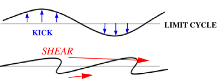
Figure 1: The stretch-and-fold action of a kick followed by relaxation in the presence of shear.

Here, the term involving $H(\theta)$ defines the kick, and $\gamma=S^{1}\times\{0\}$. We explain intuitively the significance of the quantity $\frac{\sigma}{\lambda}A$. As noted earlier, to create a strange attractor, it is necessary to “break” the limit cycle. The more strongly attractive $\gamma$ is, the harder it is to break. From this we see the advantage of having $\lambda$ small. By the same token, a stronger forcing, i.e., larger $A$, helps. The role of $\sigma$, the shear, is explained pictorially in Fig. 1: Since the function $H$ is required to be nonconstant, let us assume the kick drives some points on the limit cycle $\gamma$ up and some down, as shown. The fact that $\sigma$ is positive means that points with larger $y$-coordinates move faster in the $\theta$-direction. During the relaxation period, the “bumps” created by the kick are stretched as depicted. At the same time, the curve is attracted back to the limit cycle. Thus, the combination of kicks and relaxation provides a natural mechanism for repeated stretching and folding of the limit cycle. Observe that the larger the differential in speed in the $\theta$-direction, i.e. the larger $\sigma$, and the slower the return to $\gamma$, i.e. the smaller $\lambda$, the more favorable the conditions are for this stretch-and-fold mechanism.

1.2 Geometry and Singular Limits

In Eq. (1), the quantities $\lambda$, $\sigma$ and $A$ appear naturally. But what about in general limit cycles, where the direction of the kicks vary? What, for example, will play the role of $\sigma$, or what we called shear in Eq. (1)? The aim of this subsection is to shed light on the general geometric picture, and to explain how the dynamics of $F_{T}$ for large $T$ can be understood.

Geometry of $F_{T}$ and the Strong Stable Foliation

Let $\gamma$ be a hyperbolic limit cycle as in the beginning of Sect. 1.1. Through each $x\in\gamma$ passes the strong stable manifold of $x$, denoted $W^{ss}(x)$ [10]. By definition, $W^{ss}(x)=\{y\in M:d(\Phi_{t}(y),\Phi_{t}(x))\to 0$ as $t\to\infty\}$; the distance between $\Phi_{t}(x)$ and $\Phi_{t}(y)$ in fact decreases exponentially. Some basic properties of strong stable manifolds are: (i) $W^{ss}(x)$ is a codimension one submanifold transversal to $\gamma$ and meets $\gamma$ at exactly one point, namely $x$; (ii) $\Phi_{t}(W^{ss}(x))=W^{ss}(\Phi_{t}(x))$, and in particular, if the period of $\gamma$ is $p$, then $\Phi_{p}(W^{ss}(x))=W^{ss}(x)$; and (iii) the collection $\{W^{ss}(x),x\in\gamma\}$ foliates the basin of attraction of $\gamma$, that is to say, they partition the basin into hypersurfaces.

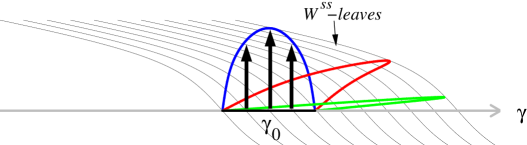
Figure 2: Geometry of folding in relation to the $W^{ss}$-foliation. Shown are the kicked image of a segment $\gamma_{0}$ and two of its subsequent images under $\Phi_{np}$.

We examine next the action of the kick map $\kappa$ in relation to $W^{ss}$-manifolds. Fig. 2 is analogous to Fig. 1; it shows the image of a segment $\gamma_{0}$ of $\gamma$ under $F_{T}=\Phi_{T}\circ\kappa$. For illustration purposes, we assume $\gamma_{0}$ is kicked upward with its end points held fixed, and assume $T=np$ for some $n\in{\mathbb{Z}}^{+}$ (otherwise the picture is shifted to another part of $\gamma$ but is qualitatively similar). Since $\Phi_{np}$ leaves each $W^{ss}$-manifold invariant, we may imagine that during relaxation, the flow “slides” each point of the curve $\kappa(\gamma_{0})$ back toward $\gamma$ along $W^{ss}$-leaves. In the situation depicted, the effect of the folding is evident.

Fig. 2 gives considerable insight into what types of kicks are conducive to the formation of strange attractors. Kicks along $W^{ss}$-leaves or in directions roughly parallel to the $W^{ss}$-leaves will not produce strange attractors, nor will kicks that essentially carry one $W^{ss}$-leaf to another. What causes the stretching and folding is the variation in how far points $x\in\gamma$ are moved by $\kappa$ as measured in the direction transverse to the $W^{ss}$-leaves. Without attempting to give a more precise characterization, we will refer to the type of chaos that results from the geometry above as shear-induced chaos. We emphasize that the occurrence of shear-induced chaos relies on the interplay between the geometries of the kicks and the underlying dynamical structures.

Returning to the concrete situation of Theorem 2, since Eq. (1) without the kick term is linear, it is easy to compute strong stable manifolds. In $(\theta,y)$-coordinates, they are lines with slope $-\lambda/\sigma$. Variations in kick distances here are guaranteed by the fact that $H$ is nonconstant. With $H$ fixed, it is clear that the larger $\sigma/\lambda$ and $A$, the greater these variations. Note that the use of the word kick “amplitude” in the statement of Theorem 2 is a little misleading, for it is not the amplitude of the kicks per se that leads to the production of chaos.

Singular Limits of $F_{T}$ as $T\to\infty$

When $T\gg 1$, i.e. when kicks are very infrequent, the map $F_{T}$ sends a small tube ${\cal U}_{T}$ around $\gamma$ back into itself. This is an example of what is called a rank-one map in [25]. Roughly speaking, a rank-one map is a smooth map whose derivative at each point is strongly contractive in all but one of the directions. Rank-one maps can be analyzed using perturbative methods if they have well-defined “singular limits.” In the context of limit cycles, these singular limits do exist; they are a one-parameter family of maps $\{f_{a}:\gamma\circlearrowleft\}$ obtained by letting $T\to\infty$ in the following way: For each $a\in[0,p)$ (recall that $p=\mbox{ period of $\gamma$}$), let

$$f_{a}(x)\ :=\ \lim_{n\to\infty}\Phi_{np+a}(\kappa(x))\qquad\mbox{ for all }x\in\gamma\ .$$ (2)

Equivalently, $f_{a}(x)$ is the unique point $y\in\gamma$ such that $\kappa(x)\in W^{ss}(y)$. Notice that $f_{a}(x)=f_{0}(x)+a\mbox{ (mod 1)}$, where we identify $\gamma$ with $[0,1]$ (with the end points identified). For Eq. (1), $f_{a}$ is easily computed to be

$$f_{a}(\theta)=\theta+a+\frac{\sigma}{\lambda}A\cdot H(\theta),$$ (3)

where the right side should again be interpreted as mod 1. (In the setting of driven oscillators, singular limits are sometimes known as “phase resetting curves”; they have found widespread use in e.g. mathematical biology [26, 9].)

It is shown in [22, 23, 24, 25] that a great deal of information on the attractor $\Gamma$ of $F_{T}$ for $T\gg 1$ can be recovered from these singular limit maps. The results are summarized below. These results hold generally, but as we step through the 3 cases below, it is instructive to keep in mind Eq. (1) and its singular limit (3), with $\frac{\sigma}{\lambda}A$ increasing as we go along:

• If $f_{a}$ is injective, i.e., it is a circle diffeomorphism, the attractor $\Gamma$ for $F_{T}$ is an invariant circle. This happens when the kicks are aimed in directions that are “unproductive” (see above), or when their effects are damped out quickly. In this case, the competing scenarios on $\Gamma$ are quasi-periodicity and “sinks,” i.e. the largest Lyapunov exponent of $F_{T}$ is zero or negative.

• When $f_{a}$ loses its injectivity, the invariant circle is “broken”. When that first happens, the expansion of the 1-D map $f_{a}$ is weak, and all but a finite number of trajectories tend to sinks. This translates into a gradient type dynamics for $F_{T}$.

• If $f_{a}$ is sufficiently expanding away from its critical points, $\Gamma$ contains horseshoes for all large $T$. For an open set of these $T$, the chaos is transient, while on a positive measure set, $F_{T}$ has a strange attractor with the properties described in Sect. 1.1. These are the two known competing scenarios. (They may not account for all $T$.) Since $F_{T}\approx F_{T+np}$ for large $T$, both sets of parameters are roughly periodic.

  The analyses in the works cited suggest that when horseshoes are first formed, the set of parameters with transient chaos is more dominant. The stronger the expansion of $f_{a}$, the larger the set of parameters with strange attractors. In the first case, the largest Lyapunov exponent of $F_{T}$ may appear positive for some time (which can be arbitrarily long) before turning negative. In the second case, it stays positive indefinitely.

1.3 Limitations of Current Analytic Techniques

In hyperbolic theory, there is, at the present time, a very large discrepancy between what is thought to be true and what can be proved. Maps that are dominated by stretch-and-fold behavior are generally thought to have positive Lyapunov exponents – although this reasoning is also known to come with the following caveat: Maps whose derivatives expand in certain directions tend to contract in other directions, and unless the expanding and contracting directions are well separated (such as in Anosov systems), the contractive directions can conspire to form sinks. This is how the transient chaos described in Sect. 1.2 comes about. Still, if the expansion is sufficiently strong, one would expect that positive Lyapunov exponents are more likely to prevail – even though for any one map the outcome can go either way. Proving results of this type is a different matter. Few rigorous results exist for systems for which one has no a priori knowledge of invariant cones, and invariant cones are unlikely in shear-induced chaos.

The rigorous results reviewed in the last two subsections have the following limitations: (i) They pertain to $F_{T}$ for only very large $T$. This is because the authors use a perturbative theory that leans heavily on the theory of 1-D maps. No non-perturbative analytic tools are currently available. (ii) A larger than necessary amount of expansion is required of the singular limit maps $f_{a}$ in the proof of strange attractors. This has to do with the difficulty in locating suitable parameters called Misiurewicz points from which to perturb. (This problem can be taken care of, however, by introducing more parameters.) We point out that (i) and (ii) together exacerbate the problem: $f_{a}$ is more expanding when $\lambda$ is small, but if $F_{T}=\Phi_{T}\circ\kappa$ is to be near its singular limit, then $e^{-\lambda T}$ must be very small, i.e. $\lambda T$ must be very large.

That brings us to the present paper, the purpose of which is to supply numerical evidence to support some of our conjectured ideas regarding situations beyond the reach of the rigorous work reviewed. Our ideas are based on the geometry outlined in Sect. 1.2, but are not limited to periodic kicks or to the folding of limit cycles.

2 Study 1: Periodically-Kicked Oscillators

Our first model is the periodic kicking of a linear shear flow with a hyperbolic limit cycle. The setting is as in Theorem 2 with $H(\theta)=\sin(2\pi\theta)$, i.e., we consider

$$\begin{array}[]{ccl}\dot{\theta}&=&1+\sigma y\ ,\\ \dot{y}&=&-\lambda y+A\cdot\sin(2\pi\theta)\cdot\sum_{n=0}^{\infty}\delta(t-nT)\ ,\\ \end{array}$$ (4)

where $(\theta,y)\in S^{1}\times{\mathbb{R}}$, $S^{1}\equiv[0,1]$ with the two end points of $[0,1]$ identified. In the absence of kicks, i.e., when $A=0$, $\Phi_{t}(z)$ tends to the limit cycle $\gamma=S^{1}\times\{0\}$ for all $z\in S^{1}\times{\mathbb{R}}$. As before, the attractor in the kicked system is denoted by $\Gamma$. The parameters of interest are:

$$\sigma =\mbox{amount of shear,}$$

$$\lambda =\mbox{damping or rate of contraction to $S^{1}\times\{0\}$,}$$

$$A =\mbox{amplitude of kicks, and}$$

$$T =\mbox{time interval between kicks.}$$

Our aim here is to demonstrate that the set of parameters with chaotic behavior is considerably larger than what is guaranteed by the rigorous results reviewed in Sect. 1, and to gain some insight into this parameter set. By “chaotic behavior,” we refer in this section to the property that $F_{T}$ has a positive Lyapunov exponent for orbits starting from a “large” set of initial conditions, i.e. a set of full or nearly full Lebesgue measure in the basin of attraction of $\Gamma$. More precisely, we assume that such Lyapunov exponents are well defined, and proceed to compute the largest one, which we call $\Lambda_{\max}$.

We begin with some considerations relevant to the search for parameters with $\Lambda_{\max}>0$:

• It is prudent, in general, to ensure that orbits do not stray too far from $\gamma$. This is because while the basin of attraction of $\gamma$ in this model is the entire phase space, the basin is bounded in many other situations. We therefore try to keep $\Gamma\subset\{|y|<b\}$ with relatively small $b$. This is guaranteed if $A$ is small enough that $e^{-\lambda T}(b+A)<b$; the bound is improved if, for example, no point gets kicked to maximum amplitude two consecutive iterates.

• Let $(\theta_{T},y_{T})=F_{T}(\theta_{0},y_{0})$. A simple computation gives

  $$\begin{array}[]{rcl}\theta_{T}&=&\theta_{0}+T+\frac{\sigma}{\lambda}\cdot[y_{0}+A\sin(2\pi\theta_{0})]\cdot(1-e^{-\lambda T})\qquad\mbox{(mod 1)}\ ,\\ y_{T}&=&e^{-\lambda T}[y_{0}+A\sin(2\pi\theta_{0})]\ .\end{array}$$ (5)

  For $b$ relatively small, we expect the number $\frac{\sigma A}{\lambda}(1-e^{-\lambda T})$ to be a good indicator of chaotic behavior: if it is large enough, then $F_{T}$ folds the annulus $\{|y|<b\}$ with two turns and maps it into itself. The larger this number, the larger the folds, meaning the more each of the monotonic parts of the image wraps around in the $\theta$-direction.

Summary of Findings.

• With the choice of parameters guided by (a) and (b) above, we find that as soon as the folding described in (b) is definite, $F_{T}$ becomes “possibly chaotic”, meaning $\Lambda_{\max}$ is seen numerically to oscillate (wildly) between positive and negative values as $T$ varies. We interpret this to be due to competition between transient and sustained chaos; see (iii) in Sect. 1.2. For larger $\frac{\sigma}{\lambda}A$, i.e., as the stretching is stronger, and for $T$ beyond an initial range, this oscillation stops and $\Lambda_{\max}$ becomes definitively positive for all the values of $T$ computed.

• As for the range of parameters with chaotic dynamics, we find that $\Lambda_{\max}>0$ occurs under fairly modest conditions, e.g., for $\frac{\sigma}{\lambda}A=3$, we find $\Lambda_{\max}>0$ starting from about $T\approx 3$, which is very far from the “$T\to\infty$” in rigorous proofs. Also, while shear-induced chaos is often associated with weak damping, we find that the phenomenon occurs as well for larger $\lambda$, e.g., for $\lambda\sim 1$, provided its relation to the other parameters are favorable.

Supporting Numerical Evidence. Figures  3 and 4 show the largest Lyapunov exponent $\Lambda_{\max}$ of $F_{T}$ versus the kick period $T$. (Note that this is the expansion rate per kick period and is $T$ times the rate per unit time.) In Fig. 3, $\lambda$ and $A$ are fixed, and $\sigma$ is increased. We purposefully start with too small a $\sigma$ so that we may see clearly the gradual changes in $\Lambda_{\max}$. The results are in excellent agreement with the description at the end of Sect. 1.2 (which pertains to regimes with very large $T$), even though $T$ is not so large here: In the top picture, where $\frac{\sigma}{\lambda}A$ is small, the plot confirms a competition between quasi-periodicity and sinks; in the middle picture, we see first $\Lambda_{\max}$ becoming increasingly negative, then transitions into a competition between transient and sustained chaos, with the latter dominating in the bottom picture. Fig. 4 shows the same phenomena in reverse order, with $\sigma$ and $A$ fixed and $\lambda$ increasing. Notice that even for $\sigma,\lambda$ and $A$ leading to chaotic dynamics, $\Lambda_{\max}$ is negative for small $T$. This is in agreement with the influence of the factor $(1-e^{-\lambda T})$ in Eq. (5).

As explained in (a) above, when $\lambda T$ is too small relative to $A$, orbits stray farther from $\gamma$. Data points corresponding to parameters for which this happens are marked by open squares. For purposes of demonstrating the phenomena in question, there is nothing wrong with these data points, but as explained earlier, caution must be exercised with these parameters in systems where the basin of $\gamma$ is smaller.

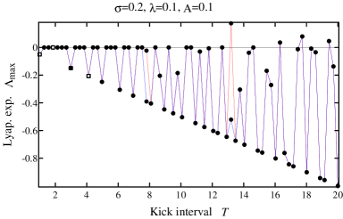
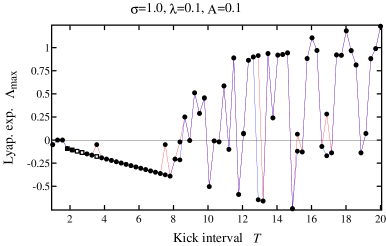
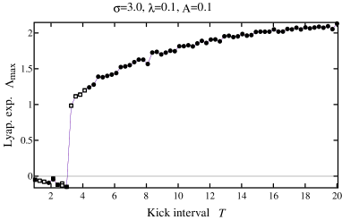
Figure 3: Effect of increasing shear on the Lyapunov exponents of the periodically-kicked linear shear flow. Squares indicate that the corresponding $F_{T}$-orbit has veered outside the region $|y|<0.15$. Upper and lower estimates of $\Lambda_{\max}$ are both shown (see Simulation Details).

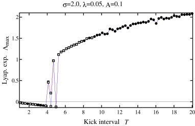
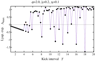
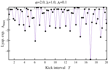
Figure 4: Effect of increasing damping on the Lyapunov exponents of the periodically-kicked linear shear flow. Squares indicate that the corresponding $F_{T}$-orbit has veered outside the region $|y|<0.15$.

Simulation Details. The numbers $\Lambda_{\max}$ are computed by iterating the map in Eq. (5) and its Jacobian, and tracking the rate of growth of a tangent vector. We use $4\times 10^{5}$ iterates of $F_{T}$ in each run. Mindful of the delicate situation due to competition between transient and sustained chaos, and to lower the possibility of atypical initial conditions, we perform 10 runs for each choice of $(\sigma,A,\lambda,T)$, using for each run an independent, random (with uniform distribution) initial condition $(\theta_{0},y_{0})\in[0,1)\times[-0.1,0.1]$. Among the 10 values of $\Lambda_{\max}$ computed, we discard the largest and the smallest, and plot the maximum and minimum of the remaining 8. As one can see in Figs. 3 and 4, the two estimates occasionally do not agree. This may be because not all initial conditions in the system have identical Lyapunov exponents, or it may be that the convergence to the true value of $\Lambda_{\max}$ is sufficiently slow and more iterates are needed, i.e. there are long transients.

3 Study 2: Poisson Kicks

We consider next a variant of Eq. (4) in which deterministic, periodic kicks are replaced by “random kicks.” Here, random kicks refer to kicks at random times and with random amplitudes. More precisely, we consider

$$\dot{\theta} =1+\sigma y$$ (6)

$$\dot{y} =-\lambda y+\sin(2\pi\theta)\sum_{n}{\bf A}_{n}\delta(t-{\bf T}_{n})$$

where the kick times ${\bf T}_{n}$ are such that ${\bf T}_{n+1}-{\bf T}_{n}$, $n=0,1,2,\cdots,$ are independent exponential random variables with mean $T$, and the kick amplitudes ${\bf A}_{n}$ are independent and uniformly distributed over the interval $[0.8\ A,1.2\ A]$ for some $A>0$. (We do not believe detailed properties of the laws of ${\bf T}$ and ${\bf A}$ have a significant impact on the phenomena being addressed.) The analog here of the time-$T$ map in Study 1 is the random map $F=\Phi_{\bf T}\circ K_{\bf A}$ where ${\bf T}$ and ${\bf A}$ are random variables.

By the standard theory of random maps, Lyapunov exponents with respect to stationary measures are well defined and are nonrandom, i.e. they do not depend on the sample path taken [12]. Notice that if $\sigma\neq 0$, the system (6) has a unique stationary measure which is absolutely continuous with respect to Lebesgue measure on $S^{1}\times{\mathbb{R}}$: starting from almost every $z_{0}\in S^{1}\times{\mathbb{R}}$, after one kick, the distribution acquires a density in the $y$-direction; since vertical lines become slanted under $\Phi_{t}$ due to $\sigma\neq 0$, after a second kick the distribution acquires a (two-dimensional) density.

In terms of overall trends, our assessment of the likelihood of chaotic behavior follows the analysis in Study 1 and will not be repeated. We identify the following two important differences:

• Smooth dependence on parameters. Due to the averaging effects of randomness, we expect Lyapunov exponents to vary smoothly with parameter, without the wild oscillations in the deterministic case.

• Effects of large deviations. A large number of kicks occurring in quick succession may have the following effects:

  • They can cause some orbits to stray far away from $\gamma=S^{1}\times\{0\}$. This is guaranteed to happen, though infrequently, in the long run. Thus, it is reasonable to require only that a large fraction — not all — of the stationary measure (or perhaps of the random attractors $\Gamma_{\omega}$) to lie in a prescribed neighborhood of $\gamma$.

  • It appears possible, in principle, for a rapid burst of kicks to lead to chaotic behavior even in situations where the shear is mild and kick amplitudes are small. To picture this, imagine a sequence of kicks sending (or maintaining) a segment far from $\gamma$, allowing the shear to act on it for an uncharacteristically long time. One can also think of such bursts as effectively setting $\lambda$ to near $0$ temporarily, creating a very large $\frac{\sigma}{\lambda}A$. On the other hand, if $\sigma$ is small, then other forces in the system may try to coax the system to form sinks between these infrequent events. We do not have the means to assess which scenario will prevail.

Summary of Findings.

In terms of overall trends, the results are consistent with those in Study 1. Two differences are observed. One is the rapid convergence of $\Lambda_{\max}$ and their smooth dependence on parameters. The other is that positive Lyapunov exponents for $F$ are found both for smaller values of $\frac{\sigma}{\lambda}A$ and for apparently very small $T$ (which is impossible for periodic kicks), lending credence to the scenario described in (b)(ii) above.

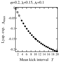
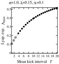
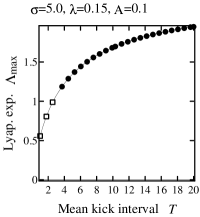
(a) Increasing shear

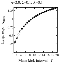
(b) Increasing damping

Figure 5: Lyapunov exponents for the linear shear flow with Poisson kicks. Squares indicate the corresponding orbit spends more than 20% of the time in the region $|y|>0.1$.

Supporting Numerical Evidence. Fig. 5 shows $\Lambda_{\max}$ as a function of the mean kick interval $T$. As in Study 1, we first show the effects of increasing $\sigma$ and then the effects of increasing $\lambda$. Without the oscillations seen previously, the present plots are straightforward to interpret. In case one wonders how $\Lambda_{\max}$ curves can switch from strictly-decreasing to strictly-increasing behavior, the middle panel of Fig. 5(b) catches such a swtich “in the act.” Squares indicate that the orbit computed spends $>20\%$ of its time outside of the region $\{|y|<0.1\}$.

4 Study 3: Continuous-Time Stochastic Forcing

In this section, we investigate the effect of forcing by white noise. The resulting systems are described by stochastic differential equations (SDEs). We consider two ways to force the system:

Study 3a: Degenerate white noise applied in chosen direction:

$$d\theta =(1+\sigma y)\ dt$$ (7)

$$dy =-\lambda y\ dt+a\sin(2\pi\theta)\ dB_{t}$$

Study 3b: Isotropic white noise:

$$d\theta =(1+\sigma y)\ dt+a\sin(2\pi\theta)\ dB^{1}_{t}$$ (8)

$$dy =-\lambda y\ dt+a\sin(2\pi\theta)\ dB^{2}_{t}$$

In Study 3a, $B_{t}$ is standard 1-dimensional Brownian motion (meaning with variance $=1$). In Study 3b, $(B^{1}_{t},B^{2}_{t})$ is a standard 2-D Brownian motion, i.e., they are independent standard 1-D Brownian motions. For definiteness, we assume the stochastic terms are of Itô type. Notice that the two parameters $A$ and $T$ in Studies 1 and 2 have been combined into one, namely $a$, the coefficient of the Brownian noise.

By standard theory [1, 13], the solution process of an SDE can be represented as a stochastic flow of diffemorphisms. More precisely, if the coefficients of the SDE are time-independent, then for any time step $\Delta t>0$, the solution may be realized, sample path by sample path, as the composition of random diffeomorphisms  $\cdots\ \circ f_{3}\circ f_{2}\circ f_{1}$, where the $f_{i}$ are chosen i.i.d. with a law determined by the system (the $f_{i}$ are time-$\Delta t$ flow-maps following this sample path). This representation enables us to treat an SDE as a random dynamical system and to use its Lyapunov exponents as an indicator of chaotic behavior. It is clear that system (8) has a unique invariant density, which is the solution of the Fokker-Planck equation. Even though the stochastic term in system (7) is degenerate, for the same reasons discussed in Study 3, it too has a unique stationary measure, and this measure has a density. The Lyapunov exponents considered in this section are with respect to these stationary measures.

Before proceeding to an investigation of the two systems above, we first comment on the case of purely additive noise, i.e. Eq. (8) without the $\sin(2\pi\theta)$ factor in either Brownian term. In this case it is easy to see that all Lyapunov exponents are $\leq 0$, for the random maps are approximately time-$\Delta t$ maps of the unforced flow composed with random (rigid) translations. Such a system is clearly not chaotic.

With regard to system (7), we believe that even though the quantitative estimates from Study 1 no longer apply, a good part of the qualitative reasoning behind the arguments continues to be valid. In particular, we conjecture that

• trends, including qualitative dependences on $\sigma$ and $\lambda$, are as in the previous two studies;

• the effects of large deviations noted for Poisson kicks (Study 2, item (b)) are even more prominent here, given that the forcing now occurs continuously in time.

As for system (8), we expect it to be less effective in producing chaos, i.e. more inclined to form sinks, than system (7). This expectation is based on the following reasoning: Suppose first that we force only in the $\theta$-direction, i.e., suppose the $dB^{2}_{t}$ term in (8) is absent. Then the stochastic flow leaves invariant the circle $S^{1}\times\{0\}$, which is the limit cycle of the deterministic part of the system. A general theorem tells us that when a random dynamical system on a circle has an invariant density, its Lyapunov exponent is always $\leq 0$; in this case, it is in fact strictly negative because of the inhomogeneity caused by the sine function [12]. Thus the corresponding 2-D system has “random sinks.” Now let us put the $y$-component of the forcing back into the system. We have seen from previous studies that forcing the $y$ direction alone may lead to chaotic behavior. The tendency to form sinks due to forcing in the $\theta$-direction persists, however, and weakens the effect of the shear-induced stretching.

We now discuss the results of simulations performed to validate these ideas.

Summary of Findings.

• In the case of degenerate white noise, the qualitative dependence of $\Lambda_{\max}$ on $\sigma$ and $\lambda$ are as expected, and the effects of large deviations are evident. In particular, $\Lambda_{\max}$ is positive for very small values of $\sigma,\lambda$ and $a$ provided $\frac{\sigma}{\lambda}$ is large. This cannot happen for periodic kicks; we attribute it to the effect of large deviations.

• Isotropic white noise is considerably less effective in producing chaos than forcing in the $y$-direction only, meaning it produces a smaller (or more negative) $\Lambda_{\max}$.

• In both cases, we discover the following approximate scaling: Under the scaling transformations $\lambda\mapsto k\lambda,\sigma\mapsto k\sigma$ and $a\mapsto\sqrt{k}a$, $\Lambda_{\max}$ transforms approximately as $\Lambda_{\max}\mapsto k\Lambda_{\max}$. In the case of degenerate white noise, when both $\sigma$ and $\frac{\lambda}{\sigma}$ are not too small (e.g., $>3$), this scaling gives excellent predictions of $\Lambda_{\max}$ for the values computed.

We remark that (iii) does not follow by scaling time in the SDE. Indeed, scaling time by $k$ in Eq. (7), we obtain

$$d\theta =(k+k\sigma y)\ dt\ ,$$ (9)

$$dy =-k\lambda y\ dt+\sqrt{k}a\sin(2\pi\theta)\ dB_{t}\ .$$

Thus the approximate scaling in (iii) asserts that the Lyapunov exponent of system (9), equivalently $k$ times the $\Lambda_{\max}$ for Eq. (7), is roughly equal to that of the system obtained by changing the first equation in (9) to $d\theta=(1+k\sigma y)dt$. In other words, $\Lambda_{\max}$ seems only to depend minimally on the frequency of the limit cycle in the unforced system.

Supporting Numerical Evidence. Plots of $\Lambda_{\max}$ as functions of $a$ are shown in Figs. 6 – 9.

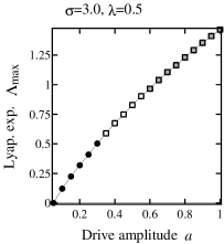
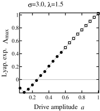
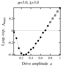
Figure 6: Lyapunov exponents for the linear shear flow driven by degenerate white noise (Eq. (7)). Open squares indicate that the corresponding orbits spend more than 20% of the time in the region $|y|>0.3$; shaded squares do the same for the region $|y|>0.5$.

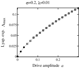
Figure 7: Lyapunov exponents for the linear shear flow driven by degnerate white noise, for small values of $\sigma$ and $\lambda$.

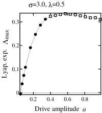
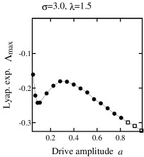
(a) $\sigma=3.0$

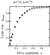
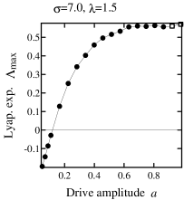
(b) $\sigma=7.0$

Figure 8: Lyapunov exponent for the linear shear flow driven by isotropic white noise (Eq. (8)). Squares indicate that the corresponding orbits spend more than 20% of the time in the region $|y|>0.3$.

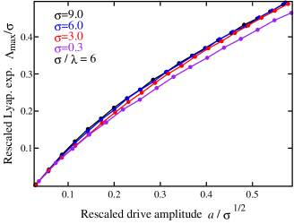
Figure 9: Evidence of scaling: We fix $\frac{\sigma}{\lambda}$ and plot $\Lambda_{\max}/\sigma$ as functions of the rescaled drive amplitude $a/\sqrt{\sigma}$; from top to bottom, the curves are in order of decreasing $\sigma$.

In Fig. 6, the forcing is degenerate, and for fixed $\sigma$, $\Lambda_{\max}$ decreases with increasing damping as expected. Notice that compared to the two previous studies, a somewhat larger damping is required to maintain a good fraction of the attractor near $\gamma$.

Fig. 7 shows that $\Lambda_{\max}$ is positive for values of $\sigma$ and $\lambda$ as small as $0.2$ and $0.01$, and white noise amplitudes $a$ close to $0$. Notice first that this is consistent with the scaling conjectured in (iii) above, and second that in the case of periodic kicks, comparable values of $\sigma$ and $\lambda$ would require a fairly substantial kick, not to mention long relaxation periods, before chaotic behavior can be produced. We regard this as convincing evidence of the significant effects of large deviations in continuous-time forcing. (It must be pointed out, however, that in our system, the basin of attraction is the entire phase space, and a great deal of stretching is created when $|y|$ is large. That means system (7) takes greater advantage of large deviations than can be expected ordinarily.

Fig. 8(a) shows $\Lambda_{\max}$ in the isotropic case for the same parameters as in Fig. 6. A comparison of the two sets of results confirms the conjectured tendency toward negative exponents when the forcing is isotropic. Fig. 8(b) shows that this tendency can be overcome by increasing $\sigma$.

Fig. 9 shows four sets of results, overlaid on one another, demonstrating the scaling discussed in item (iii) above. Fixing $\frac{\sigma}{\lambda}=6$, we show the graphs of $\Lambda_{\max}/\sigma$ as functions of $a/\sqrt{\sigma}$ for four values of $\sigma$. The top two curves (corresponding to $\sigma=6$ and $9$) coincide nearly perfectly. Similar approximate scalings, less exact, are observed for smaller values of $\frac{\sigma}{\lambda}$, both when $\Lambda_{\max}$ is positive and negative.

Simulation Details. We compute Lyapunov exponents numerically by solving the corresponding variational equations (using an Euler solver with time steps of $10^{-5}$) and tracking the growth rate of a tangent vector. To account for the impact of the realization of the forcing on the computed exponents, for each choice of $(\sigma,\lambda,a)$ we perform 12 runs in total, using 3 independent realizations of the forcing and, for each realization, 4 independent initial conditions (again uniformly-distributed in $[0,1)\times[-0.1,0.1]$). For almost all the parameter values, the estimates agree to fairly high accuracy, so we simply average over initial conditions and plot the result.

Related Results.

The asymptotic stability of dynamical systems driven by random forcing has been investigated by many authors using both numerical and analytic methods. Particularly relevant to our study are results pertaining to the random forcing of oscillators (such as Duffing-van der Pol oscillators) and stochastic Hopf bifurcations; see e.g. [2, 3, 7, 5, 6, 8, 18, 16]. Most of the existing results are perturbative, i.e., they treat regimes in which both the noise and the damping are very small. Positive Lyapunov exponents are found under certain conditions. We do not know at this point if the geometric ideas of this paper provide explanations for these results.

5 Study 4: Sheared-Induced Chaos in Quasiperiodic Flows

Model and Background Information

In this section, we will show that external forcing can lead to shear-induced chaos in a coupled phase oscillator system of the form

The governing equations are

$$\dot{\theta}_{1} =\nu_{1}+z(\theta_{1})[a_{\rm ff}g(\theta_{2})+I(t)]\ ,$$ (10)

$$\dot{\theta}_{2} =\nu_{2}+z(\theta_{2})[a_{\rm fb}g(\theta_{1})].$$

The state of the system is specified by two angles, $(\theta_{1},\theta_{2})$, so that the phase space is the torus ${\mathbb{T}}^{2}\equiv[0,1)^{2}$. The constants $\nu_{1}$ and $\nu_{2}$ are the oscillators’ intrinsic frequencies; we set $\nu_{1}=1$ and $\nu_{2}=1.1$ (representing similar but not identical frequencies). The constants $a_{\rm ff}$ and $a_{\rm fb}$ govern the strengths of the feedforward and feedback couplings. The oscillators are pulse-coupled: the coupling is mediated by a bump function $g$ supported on $[-\frac{1}{20},\frac{1}{20}]$ and normalized so that $\int_{0}^{1}g(\theta)\ d\theta=1$. The function $z(\theta)$, which we take to be $z(\theta)=\frac{1}{2\pi}[1-\cos(2\pi\theta)]$, specifies the sensitivity of the oscillators to perturbations when in phase $\theta$. Finally, we drive the system with an external forcing $I(t)$, which is applied to only the first oscillator. This simple model arises from neuroscience [26, 20] and is examined in more detail in [15].

Let $\Phi_{t}$ denote the flow of the unforced system, i.e., with $I(t)\equiv 0$. Flowlines are roughly northeasterly and are linear except in the strips $\{|\theta_{1}|<\frac{1}{20}\}$ and $\{|\theta_{2}|<\frac{1}{20}\}$, where they are bent according to the prescribed values of $a_{\rm ff}$ and $a_{\rm fb}$. Let $\rho$ denote the rotation number of the first return map of $\Phi_{t}$ to the cross-section $\{\theta_{2}=0\}$. It is shown in [14] that for $a_{\rm ff}=1$, $\rho$ is monotonically increasing (constant on extremely short intervals) as one increases $a_{\rm fb}$, until it reaches $1$ at $a_{\rm fb}=a_{\rm fb}^{*}\approx 1.4$, after which it remains constant on a large interval. At $a_{\rm fb}=a_{\rm fb}^{*}$, a limit cycle emerges in which each oscillator completes one rotation per period; we say the system is 1:1 phase-locked, or simply phase-locked. In [14], it is shown numerically that forcing the system by white noise after the onset of phase-locking leads to $\Lambda_{\max}>0$. The authors of [14] further cite Wang-Young theory (the material reviewed in Sect. 1) as a geometric explanation for this phenomenon.

In this section, we provide geometric and numerical evidence of shear-induced chaos both before and after the onset of phase-locking at $a_{\rm fb}=a_{\rm fb}^{*}$. Our results for $a_{\rm fb}>a_{\rm fb}^{*}$ support the assertions in [14]. For $a_{\rm fb}<a_{\rm fb}^{*}$, they will show that limit cycles are not preconditions for shear-induced chaos. We will show that in Eq. (10), the mechanism for folding is already in place before the onset of phase-locking, where the system is quasi-periodic or has periodic orbits of very long periods; the distinction between these two situations is immaterial since we are concerned primarily with finite-time dynamics. In the rest of this section, we will, for simplicity, refer to the regime prior to the onset of phase-locking as “near-periodic.”

Folding: Geometric Evidence of Chaos

The dynamical picture of kicks followed by a period of relaxation has a simpler, more clear-cut geometry than that of continuous, random forcing. Thus we use the former to demonstrate why one may expect chaotic behavior over the parameter ranges in question. The kick map is denoted by $\kappa$ as in Section 1.

Folding in the periodic (i.e. phase-locked) regime. We will use $a_{\rm fb}=1.47$ for illustration purposes; similar behavior is observed over a range of $a_{\rm fb}$ from $1.4$ to $1.6$. Note that the system is phase-locked for a considerably larger interval beyond $a_{\rm fb}=1.6$, but the strength of attraction grows with increasing $a_{\rm fb}$, and when the attraction becomes too strong, it is harder for folding to occur.

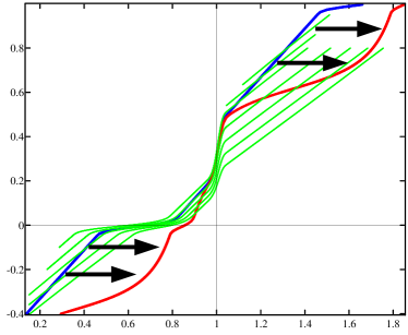
Figure 10: The strong-stable foliation of the system (10) in the phase-locked regime. Blue: a lift of the limit cycle. Red: the image of the cycle after a single kick. Green: strong-stable foliation. Here, the parameters are $\nu_{1}=1$, $\nu_{2}=1.1$, $a_{\rm ff}=1$, and $a_{\rm fb}=1.47$.

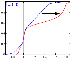
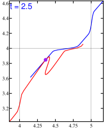
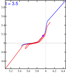
Figure 11: Snapshots of the limit cycle and its kicked image in a moving frame. Blue curves: $\Phi_{t}$-images of $\gamma_{0}$, the part of the limit cycle between $\theta_{2}=0$ and $\theta_{2}=1$. Red curves: $\kappa(\gamma_{0})$ and its images. Purple dot: the point on $\gamma_{0}$ which does not move under $\kappa$. The parameters are the same as in Fig. 10.

Fig. 10 shows the limit cycle $\gamma$ (blue curve) of the unforced system at $a_{\rm fb}=1.47$; more precisely, it shows a “lift” of $\gamma$ to ${\mathbb{R}}^{2}$, identifying the torus ${\mathbb{T}}^{2}$ with ${\mathbb{R}}^{2}/{\mathbb{Z}}^{2}$. Also shown is the image $\kappa(\gamma)$ of the cycle after a single kick (red curve), where the kick map $\kappa$ corresponds to $I(t)=A\sum_{n}\delta(t-nT)$ with $A=1.5$, i.e. $\kappa$ is given by $\kappa=\lim_{\varepsilon\to 0}\kappa_{\varepsilon}(\varepsilon)$ where $\kappa_{\varepsilon}(t)$ is the solution of $\dot{\theta}_{1}=\frac{A}{\varepsilon}z(\theta_{1}),\dot{\theta}_{2}=0$. Notice the special form of the kicks: $\kappa$ acts horizontally, and does not move points on $\theta_{1}=0$. In particular, $\kappa$ fixes a unique point $(0,b)$ on the cycle; this point is, in fact, not affected by any kick of the form considered in Eq. (10). Several segments of strong stable manifolds (green curves) of the unforced system are drawn. Recall that if $p$ is the period of cycle and $n\in{\mathbb{Z}}^{+}$, then $\Phi_{np}(\kappa(z))$ lies on the $W^{ss}$-curve through $\kappa(z)$ and is pulled toward the cycle as $n$ increases (see Sect. 1.2). From the relation between the $W^{ss}$-curves and the cycle, we see that for $z\in\gamma$, $\Phi_{t}(\kappa(z))$ will lag behind $\Phi_{t}(z)$ during the relaxation period. Notice in particular that there are points on $\kappa(\gamma)$ above the line $\theta_{2}=b$ that are pulled toward the part of $\gamma$ below $\theta_{2}=b$. Since $(0,b)$ stays put, we deduce that some degree of folding will occur if the time interval between kicks is sufficiently long.

Fig. 11 illustrates how this folding happens through three snapshots. We begin with a segment $\gamma_{0}\subset\gamma$ between $\theta_{2}=0$ and $\theta_{2}=1$ (blue curve) and its image after a single kick (red curve). Both curves are then evolved forward in time and their images at $t=2.5$ and $t=3.5$ are shown. The purple dot marks the point on $\gamma_{0}$ which does not move when kicked. Notice that these pictures are shown in a moving frame to emphasize the geometry of $\Phi_{t}(\kappa(\gamma_{0}))$ relative to $\Phi_{t}(\gamma_{0})$.

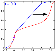
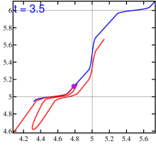
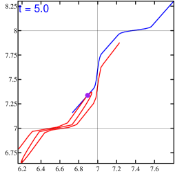
Figure 12: Snapshots of an orbit segment and its image after a single kick in a moving frame, for the system (10) in a near-periodic regime. Blue curves: a segment $\gamma_{0}$ of an orbit and its forward images $\Phi_{t}(\gamma_{0})$ at $t=3.5$, $5$. Red curves: $\kappa(\gamma_{0})$ and its forward images. Purple dot: the point on $\gamma_{0}$ which does not move under $\kappa$. The parameters are $\nu_{1}=1$, $\nu_{2}=1.1$, $a_{\rm ff}=1$, and $a_{\rm fb}=1.2$.

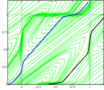
Figure 13: The time-5 stable foliation of the system (10) in a near-periodic regime. Blue & black curves: two orbit fragments. Green curves: time-5 stable foliation. The parameters here are the same as in Fig. 12.

Folding in the near-periodic regime. Fig. 12 shows snapshots of a similar kind for $a_{\rm fb}=1.2$; this value of $a_{\rm fb}$ puts the system in the near-periodic regime. The snapshots begin with an (arbitrary) orbit segment $\gamma_{0}$ and its image $\kappa(\gamma_{0})$; the location of $\gamma_{0}$ is near that of the limit cycle in Fig. 10. The kicked segment clearly folds; indeed, the picture is qualitatively very similar to that of the limit cycle case. Note that at $a_{\rm fb}=1.2$, the rotation number of the return map to $\{\theta_{2}=0\}$ is a little below 1, so that $\Phi_{t}(\kappa(\gamma_{0}))$ has an overall, slow drift to the left when viewed in the fixed frame $[0,1)^{2}$. This slow, left-ward drift is not especially relevant in our moving frame (which focuses on the movement of $\Phi_{t}(\kappa(\gamma_{0}))$ relative to that of $\Phi_{t}(\gamma_{0})$). On successive laps around the torus, the orbit in question returns to the part of the torus shown in the figure, and the sequence of actions depicted in Fig. 12 is repeated. We regard this as geometric evidence of shear-induced chaos.

We have seen that in the phase-locked regime, the folding of the limit cycle (when the time interval between kicks is sufficiently large) can be deduced from the geometry of the strong stable foliation. A natural question is: in the quasi-periodic regime, are there geometric clues in the unforced dynamics that will tell us whether the system is predisposed to chaotic behavior when forced? Since folding occurs in finite time, we believe the answer lies partially in what we call finite-time stable manifolds, a picture of which is shown in Fig. 13. We first explain what these manifolds are before discussing what they can — and cannot — tell us.

Fix $t>0$. At each $z\in{\mathbb{T}}^{2}$, let $V(z)$ be the most contracted direction of the linear map $D\Phi_{t}(z)$ if it is uniquely defined, i.e. if $v$ is a unit tangent vector at $z$ in the direction $V(z)$, then $|D\Phi_{t}(z)v|\leq|D\Phi_{t}(z)u|$ for all unit tangent vectors $u$ at $z$. A smooth curve is called a time-$t$ stable manifold if it is tangent to $V$ at all points; these curves together form the time-$t$ stable foliation. In general, time-$t$ stable manifolds are not necessarily defined everywhere; they vary with $t$, and may not stabilize as $t$ increases. When “real” (i.e. infinite-time) stable manifolds exist, time-$t$ stable manifolds converge to them as $t\to\infty$.

The blue curve in Fig. 13 is an orbit segment of $\Phi_{t}$. The angles between this segment and the time-$5$ stable manifolds (green curves) reflect the presence of shear. For example, if a kick sends points on the blue curve to the right, then within $5$ units of time most points on the kicked segment will lag behind their counterparts on the original orbit segment — except for the point with $\theta_{1}=0$ at the time of the kick. Pinching certain points on an orbit segment while having the rest slide back potentially creates a scenario akin to that in Fig. 2; see Sect. 1.2. One is also likely to find shear along the black curve in Fig. 13, a second orbit segment of $\Phi_{t}$. Whether or not the shear here is strong enough to cause the formation of folds in 5 units of time cannot be determined from the foliation alone; more detailed information such as contraction rates are needed. What Fig. 13 tells us are the mechanism and the shapes of the folds if they do form. Notice also that shearing occurs in opposite directions along the blue and black segments. This brings us to a complication not present previously: each orbit of $\Phi_{t}$ spends only a finite amount of time near, say, the blue curve before switching to the region near the black curve, and when it does so, it also switches the direction of shear. Finite-time stable foliations for system (10) have also been computed for $t\in\{3,5\}$ and a sample of $a_{\rm fb}\in(1.1,1.6)$ (not shown). They are qualitatively similar to Fig. 13, with most of the leaves running in a northeasterly direction.

In summary, for $t$ not too large, time-$t$ stable foliations generally do not change quickly with $t$ or with system parameters. They are good indicators of shear, but do not tell us if there is enough shear for folds to form. For the system defined by (10), given that the finite-time stable manifolds are nearly parallel to flowlines and the kick map acts unevenly with respect to this foliation, we conclude the presence of shear. Fig. 12 and similar figures for other $a_{\rm fb}$ (not shown) confirm that folding does indeed occur when the system is forced in the near-periodic regime.

Computation of Lyapunov exponents

To provide quantitative evidence of shear-induced chaos in the situations discussed above, we compute $\Lambda_{\max}$. Recall that while periodic kicks followed by long relaxations provide a simple setting to visualize folding, it is not expected to give clean results for $\Lambda_{\max}$ because of the competition between transient and sustained chaos (see Sect. 1.2). Continuous-time random forcing, on the other hand, produces numerical results that are much easier to interpret.

Study 4a: Stochastic Forcing.

We consider system (10) with $a_{\rm ff}=1$ and $a_{\rm fb}\in[1.1,1.6]$. The forcing is of the form $I(t)=a\cdot dB_{t}$ where $B_{t}$ is standard Brownian motion.

Study 4b: Periodic kicks.

The equation and parameters are as above, and the forcing is given by $I(t)=A\cdot\sum_{n}\delta(t-nT)$.

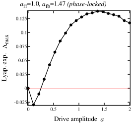
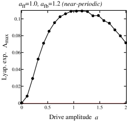
(a)	(b)

Figure 14: Lyapunov exponent of the system (10) subjected to white noise forcing. The parameters correspond to those in Figs. 10 and 12, respectively.

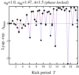
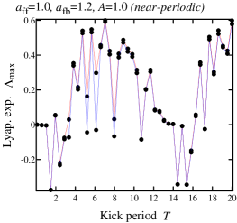
(a)	(b)

Figure 15: Lyapunov exponent of the system (10) subjected to periodic kicks. The parameters correspond to those in Figs. 10 and 12, respectively. As in Study 1, we show both upper and lower estimates of $\Lambda_{\max}$.

Summary of Findings.

Positive $\Lambda_{\max}$ are found for stochastic forcing in the parameter interval studied, both before and after the onset of phase-locking at $a_{\rm fb}=a_{\rm fb}^{*}$. For periodic kicks with large enough $A$ and $T$, it appears that $\Lambda_{\max}$ is positive for a fraction of the forcing periods tested, but the results are hard to interpret due to the competition between transient and sustained chaos.

Supporting Numerical Evidence. Fig. 14 shows some results for stochastic forcing. For $a_{\rm fb}=1.47$, negative Lyapunov exponents are found for very small amplitudes of forcing, while slightly stronger forcing (e.g. $a\approx 0.4$) is needed before $\Lambda_{\max}>0$ can be concluded with confidence. In contrast, even fairly small values of forcing seem to lead to $\Lambda_{\max}>0$ when $a_{\rm fb}=1.2$, i.e. in the near-periodic regime. This may be explained by the damping in the limit cycle case, especially for larger $a_{\rm fb}$. Notice also that in this model large amplitudes of forcing do not lead to larger $\Lambda_{\max}$. This is due to the fact that unlike the system in Studies 1–3, a very strong forcing merely presses most of the phase space against the circle $\theta_{1}=0$, which is not very productive from the point of view of folding phase space. Fig. 15 shows plots of $\Lambda_{\max}$ for periodic kicks. Here, roughly 40% of the kick periods $T$ for which Lyapunov exponents were computed yield a positive exponent. More generally, we find that $\Lambda_{\max}>0$ for over 40% of kick intervals $T$ as $A$ varies over the range $[0.75,1.5]$. See Simulation Details in Study 1.

Conclusions

Shear-induced chaos, by which we refer to the phenomenon of an external force interacting with the shearing in a system to produce stretches and folds, is found to occur for wide ranges of parameters in forced oscillators and quasi-periodic systems. Highlights of our results include:

• For periodically kicked oscillators, positive Lyapunov exponents are observed under quite modest impositions on the unforced system and on the relaxation time between kicks (in contrast to existing rigorous results). These regimes are, as expected, interspersed with those of transient chaos in parameter space.

• Continuous-time stochastic forcing is shown to be equally effective in producing chaos. The qualitative dependence on parameters is similar to that in deterministic forcing. We find that suitably directed, degenerate white noise is considerably more effective than isotropic white noise (and additive noise will not work). We have also found evidence for an approximate scaling law relating $\Lambda_{\max}$ to $\sigma$, $\lambda$, and $a$. Other types of random forcing such as Poisson kicks are also studied and found to produce chaos.

• The shear-induced stretching-and-folding mechanism can operate as well in quasi-periodic systems as it does in periodic systems, i.e. limit cycles are not a precondition for shear-induced chaos. We demonstrate this through a pulse-coupled 2-oscillator system. Chaos is induced under both periodic and white noise forcing, and a geometric explanation in terms of finite-time stable manifolds is proposed.

The conclusions in (i) and (ii) above are based on systematic numerical studies of a linear shear flow model. As this model captures the essential features of typical oscillators, we expect that our conclusions are valid for a wide range of other models. Our numerical results, particularly those on stochastic forcing, point clearly to the possibility of a number of (rigorous) theorems.

References

- [1] L. Arnold, Random Dynamical Systems, Springer-Verlag (1998)
- [2] L. Arnold, N. Sri Namachchivaya, K. R. Schenk-Hoppé, “Toward an understanding of stochastic Hopf bifurcation: a case study,” Int. J. Bifur. and Chaos 6 (1996) pp. 1947–1975
- [3] E. I. Auslender and G. N. Mil’shteĭn, “Asymptotic expansions of the Liapunov index for linear stochastic systems with small noise,” J. Appl. Math. Mech. 46 (1982) pp. 358–365
- [4] P. H. Baxendale, “A stochastic Hopf bifurcation,” Probab. Theory and Related Fields (1994) pp. 581–616
- [5] P. H. Baxendale, “Lyapunov exponents and stability for the stochastic Duffing-van der Pol oscillator,” IUTAM Symposium on Nonlinear Stochastic Dynamics, Kluwer (2003) pp. 125–135
- [6] P. H. Baxendale, “Stochastic averaging and asymptotic behavior of the stochastic Duffing-van der Pol equation,” Stochastic Process. Appl. 113 (2004) pp. 235–272
- [7] P. H. Baxendale, “Lyapunov exponents and resonance for small periodic and random perturbations of a conservative linear system,” Stoch. Dyn. 2 (2002) pp. 49–66
- [8] P. H. Baxendale and L. Goukasian, “Lyapunov exponents for small random perturbations of Hamiltonian systems,” Annals of Probability 30 (2002) pp. 101–134
- [9] J. Guckenheimer, “Isochrons and phaseless sets,” J. Theor. Biol. 1 (1974) pp. 259–273
- [10] J. Guckenheimer and P. Holmes, Nonlinear Oscillations, Dynamical Systems, and Bifurcations of Vector Fields, Springer-Verlag (1983)
- [11] J. Guckenheimer, M. Weschelberger, and L.-S. Young, “Chaotic attractors of relaxation oscillators,” Nonlinearity 19 (2006) pp. 701–720
- [12] Yu. Kifer, Ergodic Theory of Random Transformations, Birkhäuser (1986)
- [13] H. Kunita, Stochastic Flows and Stochastic Differential Equations, Cambridge University Press (1990)
- [14] K. K. Lin, E. Shea-Brown, L.-S. Young, “Reliable and unreliable dynamics in driven coupled oscillators,” preprint (2006); arXiv:nlin/0608021v1
- [15] K. K. Lin, E. Shea-Brown, L.-S. Young, “Reliable and unreliable dynamics in coupled oscillator networks,” in preparation
- [16] N. Sri Namachchivaya, “The asymptotic stability of a weakly perturbed 2-dimensional non-Hamiltonian system”, private communication
- [17] A. Oksasoglu and Q. Wang, “Strange attractors in periodically-kicked Chua’s circuit,” Int. J. Bifur. Chaos 16 (2005) pp. 83–98
- [18] M. Pinsky and V. Wihstutz, “Lyapunov exponents of nilpotent Itô systems,” Stochastics 25 (1998) pp. 43–57
- [19] K. R. Schenk-Hoppé, “Bifurcation scenarios of the noisy Duffing-van der Pol oscillator,” Nonlinear Dynamics 11 (1996) pp. 255–274
- [20] D. Taylor and P. Holmes, “Simple models for excitable and oscillatory neural networks,” J. Math. Biol. 37 (1998) pp. 419–446
- [21] B. van der Pol and J. van der Mark, “Frequency demultiplication,”Nature 120 (1927) pp. 363–364
- [22] Q. Wang and L.-S. Young, “Strange attractors with one direction of instability,” Comm. Math. Phys. 218 (2001) pp. 1–97
- [23] Q. Wang and L.-S. Young, “From invariant curves to strange attractors,” Comm. Math. Phys. 225 (2002) pp. 275–304
- [24] Q. Wang and L.-S. Young, “Strange attractors in periodically-kicked limit cycles and Hopf bifurcations,” Comm. Math. Phys. 240 (2003) pp. 509–529
- [25] Q. Wang and L.-S. Young, “Toward a theory of rank one attractors,” Annals of Mathematics (to appear)
- [26] A. Winfree, The Geometry of Biological Time, Second Edition, Springer-Verlag (2000)
- [27] G. Zaslavsky, “The simplest case of a strange attractor,” Physics Letters 69A (1978) pp. 145–147