Statistical analyses of long–term variability of AGN at high radio frequencies

Abstract

Aims. We present a study of variability time scales in a large sample of Active Galactic Nuclei at several frequencies between 4.8 and 230 GHz. We investigate the differences of various AGN types and frequencies and correlate the measured time scales with physical parameters such as the luminosity and the Lorentz factor. Our sample consists of both high and low polarization quasars, BL Lacertae objects and radio galaxies. The basis of this work is the 22 GHz, 37 GHz and 87 GHz monitoring data from the Metsähovi Radio Observatory spanning over 25 years. In addition, we used higher 90 GHz and 230 GHz frequency data obtained with the SEST-telescope between 1987 and 2003. Further lower frequency data at 4.8 GHz, 8 GHz and 14.5 GHz from the University of Michigan monitoring programme have been used.

Methods. We have applied three different statistical methods to study the time scales: The structure function, the discrete correlation function and the Lomb–Scargle periodogram. We discuss also the differences and relative merits of these three methods.

Results. Our study reveals that smaller flux density variations occur in these sources on short time scales of 1-2 years, but larger outbursts happen quite rarely, on the average only once in every 6 years. We do not find any significant differences in the time scales between the source classes. The time scales are also only weakly related to the luminosity suggesting that the shock formation is caused by jet instabilities rather than the central black hole.

1 Introduction

Long term multifrequency monitoring data of a large sample of Active Galactic Nuclei (AGNs) provides an efficient means for studying the physical processes behind the variability behaviour of individual objects. It is also a useful tool for studying differences between various AGN classes. Hughes et al. (1992) used the structure function (SF) to study the time scales of variability in a large sample of sources at frequencies 4.8, 8 and 14.5 GHz, using data from the University of Michigan monitoring programme. The SF was also used by Lainela & Valtaoja (1993), hereafter Paper I, to study the time scales of the Metsähovi monitoring sample. Since then the amount of data has more than tripled. In this paper we analyse the updated extensive database and compare the results to Paper I.

The discrete correlation function (DCF) and the Lomb–Scargle periodogram (LS–periodogram) were also used to search for the variability time scales at several frequency bands. Both of these have been used previously to study periodicities and time scales in individual sources (eg. Villata et al. 2004; Ciaramella et al. 2004; Raiteri et al. 2003, 2001; Roy et al. 2000). Aller et al. (2003) studied the Pearson-Readhead extragalactic source sample, monitored at the University of Michigan, by using the LS–periodogram without finding any significant periodicities.

We have used these methods to look for the typical flare occurrence rates and other variability properties of this large sample of sources. By using more than one method we hoped to ensure that the time scales obtained are real. Furthermore, the experience we gain in using different methods will let us choose in the future the proper methods for specific analysis needs. The DCF was used to study the radio–optical correlations in the Metsähovi monitoring sample by Tornikoski et al. (1994) and Hanski et al. (2002). In the present paper we have, however, used the autocorrelation at each radio frequency band instead of cross correlation between different frequencies.

The long term variability time scales can tell us about how often certain objects, or certain classes of objects, are in a flaring state and how long do these flares typically last. We also learn about flare evolution from one frequency domain to the other. This helps us in developing radio shock models. The knowledge of typical flare time scales is also important for the work done on extragalactic foreground sources for the ESA Planck Surveyor satellite mission, to be launched in 2008. The Planck satellite will be used to study the cosmic microwave background (CMB) emission, and all the foreground sources, including AGNs, must be removed from the results. Therefore it is important to understand the characteristic time scales of AGN variability at high radio frequencies. This paper is part of our broader study of various AGN types that affect the foreground of Planck.

This paper is organised as follows: In Sect. 2 we describe the source sample and the data. The methods used for the analyses are described in Sect. 3 and the results are presented in Sect. 4. Finally, we will discuss the scientific outcome of the results in Sect. 5. In Sect. 6 we will draw the conclusions.

2 The Sample and Observations

The sample consists of 80 sources which have been selected from the Metsähovi monitoring sample. We included objects for which we have data from a time window of over 10 years in at least two frequency bands. However, most of the sources have been monitored up to 25 years, enabling a search for longer time scales. Sources which are included in the monitoring list are bright sources with a flux density of least 1 Jy in the active state. The present sample is shown in Table LABEL:table:sourcelist. The columns show the observing frequency, the length of the time series and the number of points for each source.

The sample consists of different types of AGNs. 24 of the sources are BL Lacertae objects (BLOs), 23 Highly Polarized Quasars (HPQs), 28 Low Polarization Quasars (LPQs) and 5 Radio Galaxies (GALs). Quasars are considered to be highly polarized if their optical polarization has exceeded 3 percent at some point in the past. It is possible that some of the low polarized objects are in reality HPQs but they have not been observed in an active state. For 5 objects we had no information about their optical polarization, and they are considered LPQs in this study. When we study the statistical differences of the various groups, only BLOs, HPQs and LPQs will be considered , because of the low number of GALs in our sample. The variability of BLOs will also be studied in more detail in a forthcoming paper by Nieppola et al. (2007, in preparation for A&A).

The core of this work is the monitoring data from the 14 meter Metsähovi Radio Telescope. We have been monitoring a sample of AGNs for over 25 years at frequencies 22, 37 and 87 GHz (Salonen et al. 1987; Teräsranta et al. 1992, 1998, 2004, 2005). Our study also includes unpublished data at 37 GHz from December 2001 to April 2005. The data for BL Lacertae objects from this period are published in Nieppola et al. (2007). The observation method and data reduction process are described in Teräsranta et al. (1998). The Swedish–ESO Submillimetre Telescope (SEST) at La Silla, Chile, was used in our monitoring campaign to sample the high frequency, 90 and 230 GHz variability of southern and equatorial sources (Tornikoski et al. (1996), Tornikoski et al. 2007, in preparation for A&A). The monitoring campaign at SEST lasted from 1987 to 2003. High frequency data at 90 and 230 GHz were also collected from the literature (Steppe et al. 1988, 1992, 1993; Reuter et al. 1997). The lower frequency data at frequencies 4.8, 8 and 14.5 GHz were provided by the University of Michigan Radio Observatory (UMRAO) monitoring programme. Details of calibration and data reduction are described in Aller et al. (1985). We had sufficiently well–sampled 230 GHz data for our analysis for only 7 sources and therefore that frequency band is not used when average time scales and differences between the source classes are studied.

The median interval between the observations in individual sources varied from 31 days to 47 days at 22 and 90 GHz, respectively. At 37 GHz the median sampling rate was 41 days, but the value depends on the source. The minimum average value, 6.8 days, was at 37 GHz for the source 3C 84, which is used as a secondary calibrator in the Metsähovi observations. The minimum average for a source not used as a calibrator was 8.9 days for the source 3C273 at 37 GHz. The maximum average value, 186.4 days, was for the source 2234+282 also at 37 GHz. We also compared the sampling rates in Paper I for the 40 sources in common in our samples with sampling rates from data after 1993. At 22 GHz the difference is larger with a median of 39 days in Paper I and 19 days after 1993. At 37 GHz the median sampling rate is 31 days for both data sets. For the 40 sources not included in Paper I, the median sampling rate during the whole period was 40 days at 22 GHz and 61 days at 37 GHz.

3 Methods

Three methods were used to study the characteristic time scales of different types of AGNs: SF, DCF and LS–periodogram. We chose to use three different methods because we also wanted to study these methods in more detail, as well as the differences between them. An additional reason for using the SF analysis was to compare the results with those of the analysis done in Paper I. This way we can study how 13 years of additional data affect the time scales.

3.1 The structure function

The general description of the structure function is given by Simonetti et al. (1985). We will use only the first-order SF defined in Eq. 1,

$$D^{1}(\tau)=\left<\left[S(t)-S(t+\tau)\right]^{2}\right>$$ (1)

where $S(t)$ is the flux density at time $t$ and $\tau$ is the time lag. Our analysis follows the descriptions in Paper I and Hughes et al. (1992). Here we will only shortly describe the method.

An ideal structure function is presented in Fig. 1. It consists of two plateaus and a slope between them. The $x$-axis shows logarithm of the timelag, $\tau$, and the $y$-axis shows the logarithm of the structure function, $D(\tau)$. We can identify a time scale at the point $T_{\mathrm{max}}$ where the structure function reaches its second, higher plateau. This time scale is the maximum time scale of correlated behaviour. For lags longer than $T_{\mathrm{max}}$, we have a plateau with amplitude equal to twice the variance of the signal. The lower plateau at short timelags is equal to twice the average variance of the measurement noise for a single data point.

In addition, we can find out the nature of the process from the slope b between the two plateaus. If the lightcurve can be modelled as a white or a red noise process, then a slope of unity in the structure function implies shot noise, and a slope close to zero implies flicker or white noise. Usually the process is a mixture of these processes and the slope is something between 0 and 1. See Hufnagel & Bregman (1992) for details. If one large outburst dominates the time series, the slope may be steeper than 1. A strong linear trend or a strong periodic oscillation in the data is expected to produce a slope of 2.

In our analysis the timelag runs from 1 week to the length of the light curve. Many of the sources have been observed approximately once a week, and therefore we have chosen the lower limit to be one week. Higher frequencies (90 and 230 GHz) have usually been monitored for shorter times. We first calculated the differences squared for all the two point pairs, and then to create the structure function we averaged all the samples into 0.1 dex wide bins.

Figure 1: Ideal Structure Function

We estimated the error caused by observational uncertainties to the SF by an independent bootstrap method. For each source and frequency we created a model light curve by running over the light curve a boxcar with a length of 10 days and averaging. We tested also other averaging lengths but using much shorter values we would have not provided enough non-zero residuals for scrambling. Much longer averaging lengths would have started to average over significant variability in some sources. We then subtracted this 10-day model from each light curve and created a bank of residuals. A new simulated light curve was made by adding to each point in the model a randomly selected residual. The time sampling of the original light curve was thus preserved. This was repeated so that each residual was selected once. Using this new light curve we recalculated a new simulated SF. The procedure was repeated 1000 times. This enables us to put confidence limits to the SF, e.g. the 99% confidence limit at a given time scale was at the value where only 5 points were above or below the value. This method clearly does not require the confidence limits to be symmetric.

Results of the analysis are presented in Sect. 4 and comparison with Paper I in Sect. 5.

3.2 Discrete correlation function

Discrete correlation function was first introduced by Edelson & Krolik (1988). Hufnagel & Bregman (1992) generalized the method to include a better error estimate. The advantage of DCF compared to other correlation methods is that it is suitable for unevenly sampled data, which is usually the case in astronomical observations. Here we will describe only briefly the method and formulae used, and refer to Tornikoski et al. (1994) and Hufnagel & Bregman (1992) for details.

First we need to calculate the unbinned correlations for the time series. Note that the formulation below allows for cross correlations. This is done using Eq. 2, where $a_{i}$ and $b_{j}$ are individual points in the time series $a$ and $b$, $\bar{a}$ and $\bar{b}$ are the means of the time series, and $\sigma^{2}_{a}$ and $\sigma^{2}_{b}$ are the variances. After calculating the UDCF the correlation function is binned. The method does not define a priori the bin size so we have tested several values. If the bin size is too large, information is lost. On the other hand, if the bin size is too small, we can get spurious correlations, and the time scales may be difficult to interpret. We have chosen a bin size of 50 days for all autocorrelations. For several sources we also tested smaller bin size of 25 days but this did not make noticeable changes to the results.

$$UDCF_{\mathrm{ij}}=\frac{(a_{i}-\bar{a})(b_{j}-\bar{b})}{\sqrt{\sigma^{2}_{a}\sigma^{2}_{b}}}$$ (2)

By binning the UDCF we obtain the DCF using Eq. 3. Here $\tau$ is the time of the centre of the time bin and $n$ is the number of points in each bin. We can also calculate the error in each bin by using Eq. 4. This represents the standard deviation of the UDCF estimates within the bin.

$$DCF(\tau)=\frac{1}{n}\Sigma UDCF_{\mathrm{ij}}(\tau)$$ (3)

$$\sigma_{\mathrm{dcf}}(\tau)=\frac{1}{n-1}\left\{\Sigma\left[UDCF_{\mathrm{ij}}-DCF\left(\tau\right)\right]^{2}\right\}^{0.5}$$ (4)

A disadvantage of this method is that it does not give any exact probability value for the calculated results. The only way we can study the reliability of the method is to use simulations. The error caused by observational uncertainties have been estimated with the same bootstrap method as for SF, described in the previous section. Here we have used 10000 simulations which means that the 99% confidence limit was at the value where 50 points were above or below the value. One should note that these confidence limits represent the ambiguity caused by observational uncertainties and do not address possible questions posed by the sampling of the data. The errors obtained with this method are similar to those calculated using Eq. 4.

We also used simulated periodic data to test the capability of DCF to find real time scales and found out that it could detect all real time scales well. For our simulations we created flux density curves with strict periodicities by multiplying flares of real sources to extend over a period of 25 years. The DCF could detect the period for the simulated data with good precision. Results of the DCF analysis are presented in Sect. 4.

3.3 Lomb-Scargle periodogram

Fourier–based methods can be used for studying periodicities in light curves. We tested if these methods are also suitable for studying the characteristic variability time scales of AGNs. We have chosen the commonly used method of Lomb-Scargle periodogram for this study (Lomb 1976; Scargle 1982). It is based on the discrete Fourier-transform which has been modified for unevenly sampled data. The method searches for sinusoidal periodicities in the frequency domain. This turns out to be problematic because our light curves are not well represented by a sum of sinusoidal functions. Usually the most significant spike of the periodogram turned out to be at the time scale of the total length of the time series, and other spikes were its harmonics.

We have taken the formulae as they appear in Press et al. (1992). First we need to calculate the mean and the standard deviation of the time series. We calculated the periodogram with a sampling interval of $1/4T$ in the frequency space. Here $T$ is the total length of the time series. The upper limit to which the periodogram was calculated was $N/2T$, where $N$ is the total number of observations. In evenly spaced data this would correspond to the Nyquist frequency. Now we can calculate the Lomb-Scargle periodogram by using Eq. 3.3,

$$P_{N}(\omega) = \frac{1}{2\sigma^{2}}\frac{\left[\Sigma_{j}(a_{j}-\bar{a})\cos\omega(t_{j}-\tau)\right]}{\Sigma_{j}\cos^{2}\omega(t_{j}-\tau)}$$

$$+\frac{1}{2\sigma^{2}}\frac{\left[\Sigma_{j}(a_{j}-\bar{a})\sin\omega(t_{j}-\tau)\right]}{\Sigma_{j}\sin^{2}\omega(t_{j}-\tau)}$$

where $t_{j}$ is the date of an individual observation and $\omega$ is the frequency at which we are calculating the periodogram. $a_{j}$ is an individual data point of time series $a$, and $\bar{a}$ is the mean of the time series. $\tau$ can be calculated from Eq. 6.

$$tan(2\omega\tau)=\frac{\Sigma_{j}\sin 2\omega t_{j}}{\Sigma_{j}\cos 2\omega t_{j}}$$ (6)

A false alarm probability level of $z\approx\ln(N/p)$ for a 99.9% for the most significant spike can be calculated (Scargle 1982). Unfortunately, this does not tell anything about the significance of other spikes in the periodogram and therefore only the most significant one is used in this analysis. In radio data the annual gaps in the data are much shorter than in the optical and do not contribute to aliasing in a significant way creating spurious spikes.

4 Results

4.1 Results of the structure function analysis

We used the structure function to study the characteristic time scales of 80 sources at frequencies 4.8, 8, 14.5, 22, 37, 90 and 230 GHz.

In total we calculated 411 structure functions from which we could determine 447 time scales. In 39 cases we could not determine a variability time scale because the function was too flat or because the errors in the structure function were too large. In 60 cases we could only get a lower limit for the time scale. We could also determine more than one time scale in 69 cases.

The relative number of sources for which we could not determine a time scale depended on the frequency, for example at 14.5 GHz we had only two such cases (sources 1147+245 and 0446+112), but at 90 GHz one third of the sources failed to provide us with a good estimate for the time scale. This was mainly due to the undersampling at 90 GHz and especially at 230 GHz, which caused the structure functions to have large errors and therefore to be difficult to interpret. Also there were only five sources with data at 230 GHz.

Also the number of the lower limit estimates varied between the frequency bands and the source classes. In Table 1 the number of such sources is written in parenthesis for each frequency band and class. The relative percentage of lower limit time scales in LPQs, BLOs and HPQs were 24%, 13% and 11%.

We have plotted the distributions of the time scales at different frequencies and source classes in Fig. 2. The median time scales of each class in the histograms are marked by vertical lines. The average and median time scales are presented in Table 1.

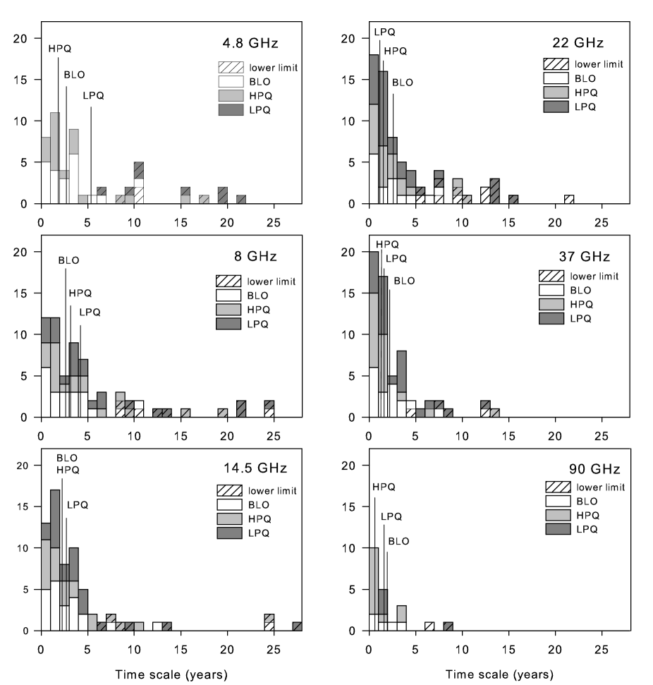
Figure 2: Distributions of time scales from structure function analysis at all frequency bands and source classes. The median values for each source class are shown by vertical lines. The time scales are in the observer’s frame.

Table 1: Averages and median values of the Structure Function analysis. Number of sources, for which only a lower limit time scale could be determined, is written in parenthesis.

Freq	type	ALL	number	BLO	number	HPQ	number	LPQ	number
		[years]	of sources	[years]	of sources	[years]	of sources	[years]	of sources
4.8	average	5.2	66(12)	3.6	23(2)	4.2	19(2)	7.8	20(8)
	redshift corr.	2.6	65	2.8	22	2.1	19	3.8	20
	median	3.0	66	2.7	23	1.9	19	5.3	20
	redshift corr.	1.7	65	1.8	22	1.0	19	1.9	20
8	average	5.6	70(13)	4.2	23(3)	4.8	20(4)	7.0	22(6)
	redshift corr.	3.5	69	3.4	22	2.4	20	3.6	21
	median	3.2	70	2.7	23	3.1	20	4.1	22
	redshift corr.	1.8	69	1.7	22	1.6	20	1.8	21
14.5	average	4.3	70(8)	3.7	23(1)	4.0	21(3)	4.5	22(4)
	redshift corr.	2.7	69	3.0	22	2.0	21	2.2	22
	median	2.3	70	2.2	23	2.2	21	2.7	22
	redshift corr.	1.3	69	1.3	22	0.8	21	1.2	22
22	average	4.1	74(14)	5.0	21(6)	2.9	20(2)	2.1	28(6)
	redshift corr.	2.5	73	4.1	20	1.3	20	1.9	28
	median	1.9	74	2.7	21	1.5	20	1.1	28
	redshift corr.	1.1	73	2.4	20	0.7	20	1.1	28
37	average	2.6	66(6)	2.8	19(2)	2.0	19(1)	3.9	23(3)
	redshift corr.	1.5	65	2.1	18	1.1	19	1.4	23
	median	1.4	66	2.2	19	1.2	19	1.5	23
	redshift corr.	0.7	65	1.3	18	0.5	19	0.8	23
90	average	2.0	23(2)	2.5	6(1)	1.1	11(0)	3.2	4(1)
	redshift corr.	1.3	23	1.8	6	0.6	11	1.9	4
	median	1.1	23	2.0	6	0.7	11	1.6	4
	redshift corr.	0.6	23	1.2	6	0.4	11	1.1	4

Because a substantial number of time scale estimates are lower limits, a much better representative for a characteristic time scale is the median time scale of the group. Practically all median time scales have value of less than 5 years. The median time scales also shorten on average with increasing frequency.

To provide a measure of the slope of the structure function between the plateaus we calculated the local slope in each structure function using trains of 2, 11 and 20 points. By comparing the plots of slope vs. time scale we estimated the actual slope for each light curve. The 2 point slope provided a local measure of the slope, while for the overall slope between the plateaus, the 11 point or the 20 point trains gave more reliable results. Which of the two was better depends on the distance of the plateaus in $\log\tau$. This was possible in 358 cases. The slopes varied from 0 to 2.2 while the average of all the frequency bands was near 1, which is expected if the light curve can be modelled as a $1/f^{2}$-type shot noise. At 37 GHz the average slope was 0.72 and at 22 GHz 0.83. We ran the Kruskal-Wallis analysis to see if there were differences between the slopes of the source classes. (All Kruskal-Wallis analyses in this paper have been performed with the Unistat software, version 5.0.) At 4.8 GHz we found that the BLOs differed from other classes significantly at P$>$95% level. At 22 GHz the HPQs differed from the BLOs significantly. At other frequencies we could not find any statistically significant differences between the groups.

4.2 Results of the DCF analysis

We used the Discrete Correlation Function to calculate the autocorrelation for 80 sources and obtained 411 autocorrelations. For many sources, more than one time scale was present in the DCF. For each we determined two time scales wherever possible. We identify as the most significant time scale the one that shows significant positive correlation after the DCF has been on the negative side. We were able to determine 273 such time scales. We also identified a time scale that we call the shortest time scale. This is the first peak in the correlation function before it has gained negative values. It did not occur in all cases and usually they appeared as small bumps in the DCF. We could determine the shortest time scale in 175 cases. Furthermore we calculated a redshift corrected time scale of the most significant time scale. Figure 3 shows the distribution of time scales at different frequency bands and source classes.

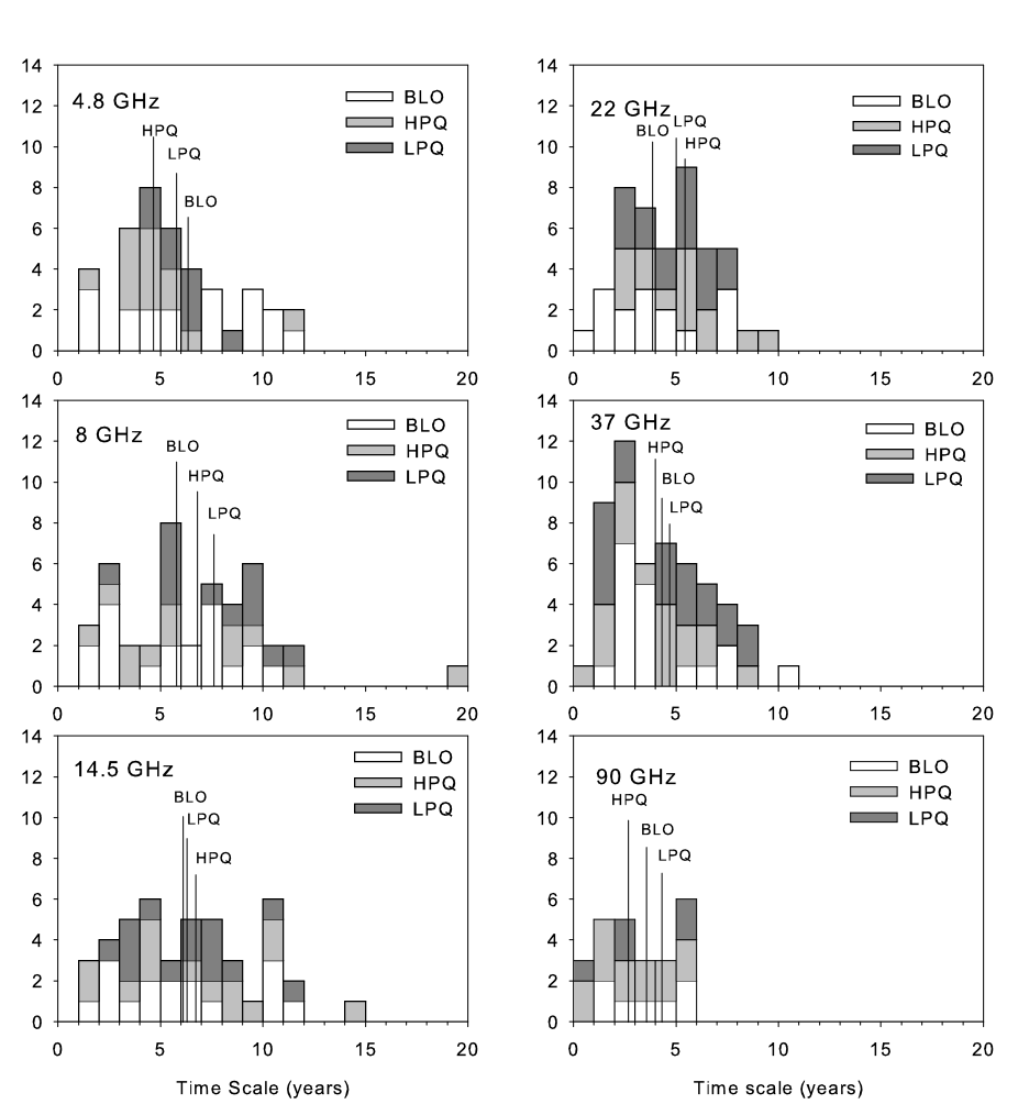
Figure 3: Distributions of the most significant DCF time scales at all frequency bands. The averages of each source class are shown by vertical lines. The time scales are in the observer’s frame.

Table 2: Averages of DCF analysis time scales. For each frequency band the most significant, shortest and redshift corrected most significant time scale averages are shown.

Freq	type	ALL	number	BLO	number	HPQ	number	LPQ	number
		[years]	of sources	[years]	of sources	[years]	of sources	[years]	of sources
4.8	most signif.	5.9	42	6.3	18	4.7	13	5.9	8
	shortest	2.3	35	2.3	13	2.1	9	2.3	11
	redshift corr.	4.0	41	4.7	17	2.6	13	3.4	8
8	most signif.	6.7	45	5.9	19	6.9	12	7.6	12
	shortest	2.0	25	1.8	10	1.9	7	2.4	8
	redshift corr.	4.1	44	4.2	18	4.2	12	3.6	12
14.5	most signif.	6.5	48	6.1	16	6.8	14	6.2	14
	shortest	1.9	31	2.3	11	1.9	11	1.9	8
	redshift corr.	4.0	47	4.4	15	3.6	14	3.1	14
22	most signif.	4.8	49	3.9	15	5.3	14	5.0	16
	shortest	1.5	35	1.4	11	1.4	7	1.6	14
	redshift corr.	2.9	48	2.9	14	2.7	14	2.7	14
37	most signif.	4.2	58	4.2	18	4.0	17	4.7	19
	shortest	1.9	35	1.6	8	2.2	10	1.8	14
	redshift corr.	2.6	57	3.2	17	2.0	17	2.4	19
90	most signif.	3.1	26	3.5	7	2.8	13	4.2	5
	shortest	1.1	12	1.1	3	1.2	6	1.1	2
	redshift corr.	1.9	26	2.3	7	1.6	13	1.6	5

Table 2 shows the average time scales from the DCF analysis for the different frequency bands, and also for BLOs, HPQs and LPQs separately at each frequency band.

4.3 Results of the Lomb-Scargle periodogram analysis

We also calculated the Lomb-Scargle periodogram for our source sample. Altogether we obtained 411 periodograms. On average we have data at 5 different frequency bands for each source. From these periodograms we found 140 time scales. In other cases there were no significant spikes in the periodogram or the spikes were at time scales over half of the total length of the time series. We did not take these into account because we are interested in time scales that have occurred at least twice during the observing period. In Fig. 4 we have plotted histograms of the distribution of time scales at all the frequency bands and for all the source classes.

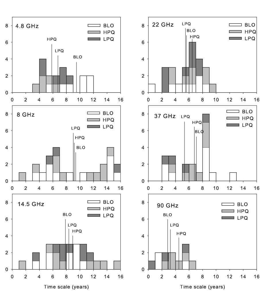
Figure 4: Distributions of most significant LS–periodogram time scales at all frequency bands. Averages of each class are shown by vertical lines. The time scales are in the observer’s frame.

We have calculated the average time scales at all the frequency bands. These are shown in Table 3. We present the results for the whole sample and also separately for BLOs, HPQs and LPQs. For each source class also the number of sources used to calculate the average are given. Each frequency band is listed separately, and the averages of the most significant time scales are shown as well as the redshift corrected time scales.

Table 3: Averages of the periodogram time scales. For each frequency band the most significant observational and redshift corrected time scale averages are given.

Freq	type	ALL	number	BLO	number	HPQ	number	LPQ	number
		[years]	of sources	[years]	of sources	[years]	of sources	[years]	of sources
4.8	most signif.	7.6	20	9.4	7	5.9	6	6.7	6
	redshift corr.	4.6	20	6.2	7	2.9	6	3.6	6
8	most signif.	9.2	25	9.4	11	9.1	10	9.0	3
	redshift corr.	5.6	25	6.4	11	5.3	10	3.8	3
14.5	most signif.	8.5	29	7.9	9	8.9	9	8.3	8
	redshift corr.	5.4	29	5.6	9	5.5	9	4.0	8
22	most signif.	5.8	28	5.6	8	6.4	8	5.4	9
	redshift corr.	3.9	28	4.7	8	3.6	8	3.0	9
37	most signif.	6.3	24	7.1	9	6.8	8	5.2	4
	redshift corr.	4.3	24	5.6	9	3.7	8	3.3	4

4.4 Differences between frequency bands and classes

We ran a set of Kruskal-Wallis tests to search for statistically significant differences between the individual frequency bands and classes. The analysis was done for all three analysis methods separately. Significant differences between frequencies were found from the results of all analysis methods.

In all cases the lower frequencies from 4.8 to 14.5 GHz formed one group. In the same way 22 and 37 GHz formed their own group. In addition there were groups with only higher frequency data from 22 GHz upwards, including 90 and 230 GHz or a group with either 22 or 37 GHz with 4.8 GHz.

We did not find significant differences between the classes in most of the frequency bands. In SF analysis only at 4.8 GHz LPQs differed from the other classes significantly. Also in LS–periodogram we could find differences only at 4.8 GHz, but this time it was the HPQs and BLOs which were drawn from different populations. In the DCF analysis we did not find any significant differences between the source classes.

4.5 Redshift corrections

We have made redshift corrections for the time scales of all those sources in our sample for which we could find a redshift in the literature. We did not have the redshift for only one BL Lac object, and for two other BLOs we had only a lower limit estimate. The redshift corrected averages for the analyses are shown in Tables 1, 2 and 3

In the SF analysis we found that at 22 and 37 GHz, the BLOs and the HPQs were drawn from different populations. At other frequency bands we did not find any significant differences. In the DCF analysis at 4.8 GHz the HPQs and BLOs differed from each other and at 37 GHz the BLOs differed from both quasar types significantly. In the LS–periodogram the results were quite similar, only at 4.8 GHz could we find any significant differences with BLOs differing from quasars. The results indicated that there may be a difference between the quasars and BLOs also at other frequency bands but there were only a few objects in each class and we would need more objects to draw conclusions about the differences. For example at 37 GHz the probability for HPQs and LPQs being from the same population was much higher than the probability of BLOs being from the same population with either of them.

4.6 Correlations

We have studied the correlation between the redshift corrected time scales from DCF analysis and different jet parameters including the Lorentz factor, the Doppler boosting factor and the viewing angle. We have taken the values from Lähteenmäki & Valtaoja (1999), where the different parameters have been calculated for 81 sources. The Doppler boosting factors are calculated from total flux density variations and for each source the flare with the highest intrinsic brightness temperature is chosen (Lähteenmäki et al. 1999). This usually means strong and rapid flares.

The samples have 64 sources in common and for those sources we used the Doppler boosting factors provided. The Lorentz factors and viewing angles were calculated for 41 sources in common with our sample. In our calculations of the luminosities we have used the same cosmology as in Lähteenmäki & Valtaoja (1999) with $\mathrm{H_{0}}=100\mathrm{kms^{-1}Mpc^{-1}}$ and $\mathrm{q_{0}}=0.5$.

We have not corrected the time scales for Doppler boosting, because the time scales from DCF analysis are time intervals between the flares and therefore Doppler boosting should not affect them.

Figure 5 shows Lorentz factor against the time scale from DCF analysis at 37 GHz. We had 30 sources for which both the Lorentz factor and the time scale were determined. We calculated the Spearman Rank Correlation and found a significant correlation of $r=-0.37$ between the parameters. There was, however, one source (2021+614) affecting the correlation with a very small Lorentz factor of 1.12. Ignoring this source made the correlation insignificant. We have also made a linear fit to the log-log values of the data by using ordinary least-squares bisector, suitable for data with both X and Y errors unknown (Isobe et al. 1990). The slope from the fit is -0.87 which would indicate that the time scales t are related to the Lorentz factor $\Gamma$ as $\mathrm{t}\propto\Gamma^{-1.2}$.

A similar fit can be made for the Doppler boosting factors and the time scales (Fig. 6) using 53 sources at 37 GHz. The result is quite surprising, a dependence with a slope of -1.1 is found implying a relation of $\mathrm{t}\propto\mathrm{D}^{-0.93}$. The correlation coefficient is $r=-0.41$, which is significant at P$>$99% level.

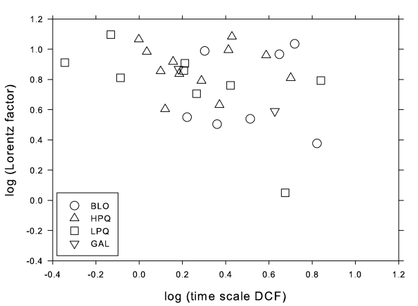
Figure 5: Correlation between the Lorentz factors and the time scales from DCF analysis at 37 GHz.

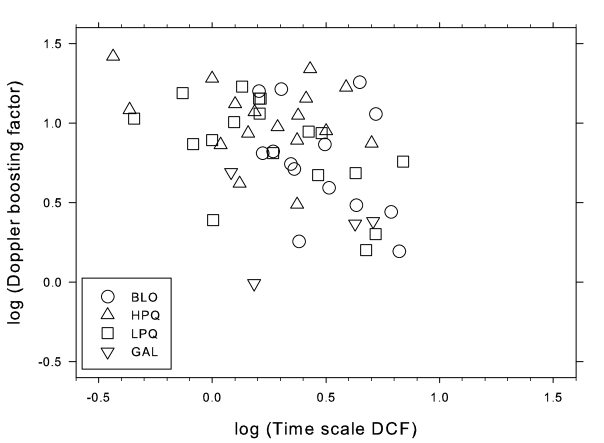
Figure 6: Correlation between the Doppler factors and the time scales from DCF analysis at 37 GHz.

The correlation between the absolute luminosity of the source and intrinsic time scales at 37 GHz is shown in Fig. 7. The correlation coefficient is $r=-0.39$, which is significant at 99% level. We obtain a slope of -2.8 from the linear fit resulting in a relation of $\mathrm{t}\propto\mathrm{L}^{-0.35}$ between the time scale t and the luminosity L of the source.

According to the standard model, Doppler boosting also affects the luminosity. Figure 8 shows the D² corrected luminosity against the time scale. The relation we obtain from a linear fit is $\mathrm{t}\propto\mathrm{L}^{-0.46}$. The correlation coefficient is $r=-0.33$, which is significant at 99% level.

We do not find any significant correlation between the viewing angle and the time scales.

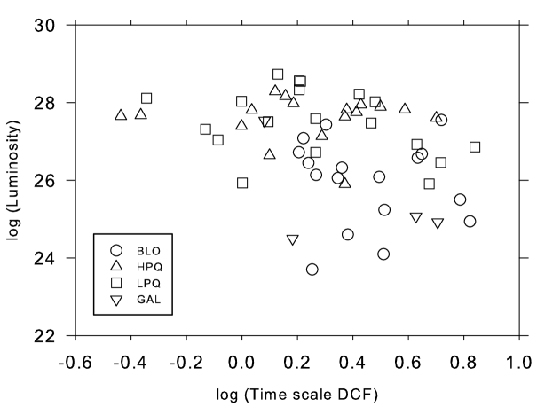
Figure 7: Correlation between the absolute luminosity and the time scale from DCF analysis at 37 GHz.

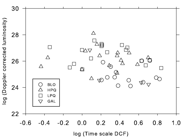
Figure 8: Correlation between the Doppler corrected absolute luminosity and the time scales from DCF analysis at 37 GHz.

We got quite similar results when we made the fits for 22 GHz data. The slopes were slightly different and also the number of sources for which we had both the parameter and the time scale determined was lower. Therefore we consider the 37 GHz results more reliable.

5 Discussion

5.1 Comparison of the structure function analyses

We have compared the results from these analyses with the results from Paper I. Table 4 lists the slopes and time scales for the 40 sources that were common to both studies. Two of the sources in the sample of Paper I are not included in this paper, because they had not been monitored intensively after 1993. In some cases the slope was complicated, and a representative value of the slope is appended with an index c.

Table 4: Parameters of the Structure Functions. Slopes which were complicated or more difficult to determine are marked with letter c. Those for which we were unable to determine the slope or the time scale are marked with -. Time scales are given in years.

Name	22 GHz	22 GHz	22 GHz	22 GHz	37 GHz	37 GHz	37 GHz	37 GHz
	b	b old	$T_{\mathrm{max}}$	$T_{\mathrm{max}}$ old	b	b old	$T_{\mathrm{max}}$	$T_{\mathrm{max}}$ old
0007$+$106	1.2	1.2	1.08	1.06	0.9	0.9	2.15	1.78
0106$+$013	0.9	1.4	2.42	$>6.68$	0.8	1.4	1.36	$>8.41$
0133$+$476	$1^{c}$	0.7	$>9.62$	2.11	0.5	0.8	0.76	1.68
0235$+$164	1.1	1.5	0.96	0.94	0.8	1	2.71	0.94
0248$+$430	0.4	2.1	$>13.58$	$>5.62$	0	2.3	-	$>7.50$
0316$+$413	1.8	1.5	$>21.53$	$>9.44$	2	1.5	3.83	3.76
0333$+$321	0.6	0.8	1.92	$>3.76$	0.7	0.9	1.21	1.06
0355$+$508	1.2	1.5	7.64	$>10.59$	$1.6^{c}$	1.7	$>12.11$	$>9.44$
0420$-$014	$0.9^{c}$	0.9	4.3	1.06	1	0.8	1.36	1.68
0422$+$004	0.6	1	$>9.62$	$>4.22$	0.6	1.5	2.71	$>4.22$
0430$+$052	1.1	0.8	0.43	0.6	1	0.7	0.54	1.5
0458$-$020	1	1.2	$>9.62$	0.67	$1^{c}$	1.3	1.71	1.88
0642$+$449	0.6	-	$>7.64$	1	0.4	0.9	$>8.57$	2.99
0735$+$178	1.3	1	6.07	4.22	1	1.1	2.15	3.76
0736$+$017	1.4	0.7	0.22	1.19	1.4	0.9	0.27	0.53
0754$+$100	1	1	0.54	1.88	0.6	1.3	1.21	1.5
0851$+$202	$0.9^{c}$	1	0.3	0.42	0.7	1.1	0.48	0.11
0923$+$392	1.3	1.3	$>13.58$	$>10.59$	1.4	1.3	5.41	$>5.31$
1055$+$018	1.2	1.2	1.36	$>9.44$	0.8	0.9	1.21	$>10.59$
1156$+$295	0.9	1.1	1.21	$>6.68$	1	2.1	1.36	$>4.73$
1219$+$285	0.3	1.1	$>21.53$	$>10.59$	0.4	1.8	4.3	$>9.44$
1226$+$023	1.3	1.4	1.36	1.5	1.3	1.5	1.21	1.19
1253$-$055	$1.2^{c}$	2.4	0.54	0.67	0.9	1.5	0.76	0.75
1308$+$326	0.8	1	2.71	3.35	0.8	1	3.04	3.73
1418$+$546	0.5	-	$>7.64$	-	0.4	1.1	0.61	0.94
1510$-$089	1	0.9	0.3	1.33	1	1	0.61	1.19
1538$+$149	0.4	1.6	$>7.64$	$>7.50$	0.4	3.9	$>7.64$	$>7.50$
1633$+$382	0.8	2.3	1.52	2.37	0.9	0.7	1.52	$>8.41$
1641$+$399	1.1	1.2	1.36	1.33	1.2	1.4	1.36	1.19
1741$-$038	1.2	1.3	1.36	$>4.22$	0.6	1.4	3.83	$>4.22$
1749$+$096	1.2	0.7	0.61	$>5.96$	1.2	0.6	0.34	$>10.59$
1807$+$698	0.2	-	-	-	0	-	-	-
2005$+$403	0.8	0.9	$>13.58$	$>10.59$	0.9	0.9	6.07	$>9.44$
2134$+$004	0.4	1.2	1.92	$>5.96$	0.4	1.3	3.41	3.76
2145$+$067	1.3	0.9	1.36	$>4.22$	1	0.8	1.36	$>4.22$
2200$+$420	$0.9^{c}$	1.1	2.42	0.67	0.9	1.1	0.48	0.38
2201$+$315	1.3	1.5	1.52	$>2.99$	1.2	1.5	3.41	$>3.76$
2223$-$052	1	1.3	2.71	1.5	1	1.5	3.04	1.06
2230$+$114	1.2	0.7	1.71	0.53	0.8	1.2	6.07	0.38
2251$+$158	0.9	1	2.15	2.37	1	1.5	0.54	0.53

We had a total of 75 source/frequency combinations where the slope and the time scale, or at least its lower limit, were determined from both analyses. Many sources had changed their behaviour during the years so that the results in the two studies differed greatly from each other. This indicates that even 10 years of monitoring is not enough to reveal the true nature of all the sources. There were also sources whose behaviour had stayed the same during the 25 years. In 20 cases the time scale had changed less than one year between the two studies and the slope had changed less than 0.3. In a total of 35 cases the time scale had changed less than a year. In 44, slightly more than half of the cases, the slope had changed $\leq 0.3$. In 21 cases the time scale had changed more than 3 years, but four of these were sources for which only a lower limit estimate could be determined in both analyses. In those cases the longer observing period caused the time scale to change more even though the behaviour of the source had not changed.

Paper I had 32 cases which gave only a lower limit for the variability time scale. In our analysis the number was reduced to fourteen. This is not unexpected as the total observing time in the present study is twice as long as in the previous analysis.

The time scales in our analysis are in general shorter than in Paper I. At 22 GHz the median value had changed from 3.0 to 1.9 years and at 37 GHz from 3.0 to 1.4 years. This can be partially explained with the smaller number of lower limit estimates in our analysis than in Paper I. Also, there are many sources that exhibit much more dramatic variability behaviour in the data set obtained after Paper I. Naturally there are also sources for which exactly the opposite is true, but because the SF determines the shortest time scale from the complete data sets, we now obtained altogether a larger number of short timescales than in Paper I. The time scales at 37 GHz are also shorter than those at 22 GHz, possibly indicating that some faster flux density variations are not clearly distinguishable at lower frequencies, including 22 GHz.

The average values for the slopes in our analysis were close to unity, typical for shot noise. At 22 GHz the average slope is 0.96 and at 37 GHz 0.86. These are slightly smaller than the values in the previous paper, where the average at 22 GHz was 1.2 and at 37 GHz 1.3. The difference between the slopes in our analysis and Paper I was significant at the 99% level. Paper I predicted that the number of very steep structure functions should be smaller with longer monitoring because usually such sources have few prominent outbursts which dominate the structure function. This effect should be smaller after longer monitoring with more flares seen in the flux density curves. This can be clearly seen from our analysis where there are only two sources with a slope over 1.5 whereas in Paper I there were 13 sources with a slope $\geq$1.5.

We did not find statistically significant differences in the time scales between the source classes LPQ, HPQ and BLO. The results in paper I suggested a statistically significant difference in the time scales of LPQs and HPQs, but we cannot confirm this.

5.2 Comparison of the time series analysis methods

We also compared the different methods used for studying the time scales. The structure function gives a different time scale compared to the other two methods. The structure function focuses on the characteristic time scales of the flux density variations, for example, the rise and decay times of the flares. Similar conclusion was made by Tanihata et al. (2001) where they used the SF method for studying the X-ray flares of AGNs. The DCF and the periodogram focus more on the periodicity and quasi-periodicity in the flux density curves and are more affected by the time cycle of the large outbursts. We could also use the SF to study the time scales between the flares by examining the first minimum in the second plateau of the SF instead of the point where the plateau starts. The minima are usually easier to see if the SF is plotted in linear scale. Here we have compared the SF time scales with Paper I and therefore used the logarithmic scale and the different time scale.

When examining the flux density curves, the time scales obtained from the DCF or the LS–periodogram could usually be identified with the time intervals between some large flares. This is also why the time scales from the DCF and the LS–periodogram are longer than the ones obtained from the structure function analysis. There is usually some variation in the flux density levels also in the short time scales but the big outbursts occur quite rarely as can be seen from the averages of the DCF and the LS–periodogram analysis.

The time scales are shorter at 4.8 GHz than at 8 GHz with every method we used. This can be due to lower flux density levels. According to the general shock model (for example Valtaoja et al. 1992), the flares last longer at the lower frequencies and the growing and decaying shocks overlap, forming a smoother curve. The flare peaks are not as extreme as at higher frequencies, and the statistical methods catch smaller peaks. Another explanation could be that the 8 GHz band has been monitored for longer periods than the 4.8 GHz band. The time scales are therefore longer, because we see more large events in the flux curves and they occur more rarely.

We could determine both a DCF and a LS–periodogram time scale in 136 cases. In one third of the cases the methods gave the same result within 0.5 years. In half of the cases the difference in the time scales was less than a year.

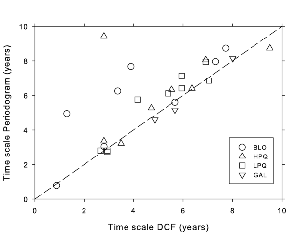
Figure 9: Time scales from the LS analysis plotted against the time scales from the DCF analysis at 22 GHz. Time scales are equal on the dashed line.

In Fig. 9 we have plotted the most significant time scale from the LS analysis against the time scale from the DCF analysis at 22 GHz. There is clearly a linear one-to-one correspondence between the time scales. There are also a few time scales above the line, and in these cases the DCF gives a shorter time scale. In all of these cases the DCF shows multiple correlations and time scales. In every case the DCF shows another time scale within a year of the periodogram time scale, but has it not been the first correlation, which was our criterion for the DCF time scale, it is not taken into account. Therefore we can conclude that the two methods give very similar results.

Figure 10: Time scales of the SF analysis plotted against the time scales of the DCF at 22 GHz. Time scales for which the structure function could only determine a lower limit are marked with crosses. The lower limits of time scales in the upper part are from left to right 12.1, 12.1, 10.8 and 21.5 years. Dashed line shows the SF time scale equals half of the DCF time scale line.

In Fig. 10 we have plotted time scales from the SF analysis against the time scales from the DCF analysis. The lower limits of time scales from SF analysis are plotted using crosses. When ignoring these time scales we can see that the SF time scales are one half of the DCF time scales or shorter. This is expected since the SF should see the rise and decay times of flares whereas the DCF sees the time interval between them or the total length of the flare.

The differences can be explained with a following example: We have a pure noiseless sinusoid with a period of $P$. The frequency $(1/P)$ found by the periodogram gives us a direct measure of the period. This is the time scale at which all the power of the variability is focused. In a DCF one is searching for a maximum correlation beyond the trivial timelag of $\tau=0$. Such a maximum is found at $\tau=P$, and all integer multiples of $P$. This is a time scale that is in full agreement with the one obtained from the periodogram. In a structure function the philosophy for the search of the time scale is somewhat different. Here we are searching for a time scale at which a maximum difference between the original and the time lagged light curves are found. For a periodic function this is reached when the timelag is $\tau=P/2$. Note that at a time scale $\tau=P$, in our simple example a deep minimum is achieved in the SF, but in reality this is filled to some extent by noise and other non-period features.

The fact that the SF is interpreted in a way to measure the maximum of the variance whereas DCF and periodogram measure the minimum in variance explains the factor 2 difference in the estimated time scales. Our data does not have strict periods, but still the different nature of the analyses reflect the property that periodogram and DCF give more characteristic measures of the times between the outbursts whereas the SF measure the rise/decay time scales, and thus a factor of 2 or larger is expected in the ratio of the estimated time scales.

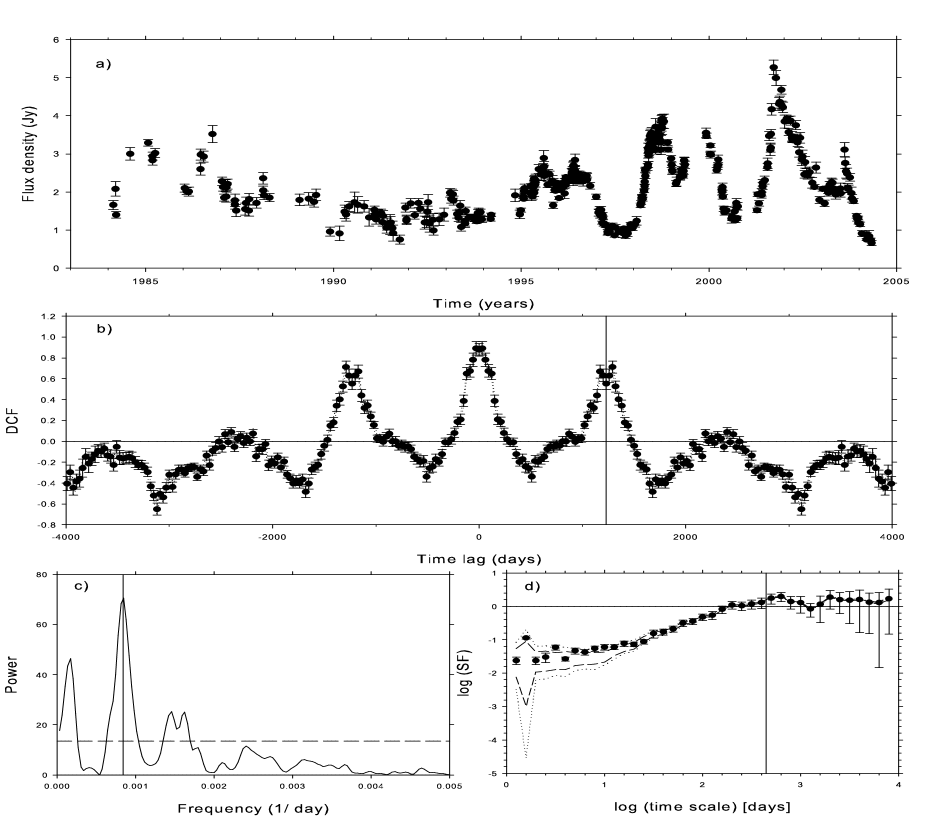
Figure 11: Analyses of the HPQ source 1156+295 at 22 GHz. a) Flux Density curve. b) The discrete correlation function. The 99.5% significance level is shown with dotted line. c) The Lomb-Scargle periodogram. Dashed line shows the false-alarm probability. d) The structure function. Dashed and dotted lines show the 97.5% and 99.5% significance levels. Time scales obtained with each method are marked by vertical lines. The most significant spike of the periodogram is at time scale of 3.29 years, which is 0.2 years shorter than the first correlation in the DCF at 3.49 years. The SF gives a time scale of 1.21 years.

As an example, Fig. 11 shows the results of all analysis methods for a HPQ source 1156+295 (4C29.45). This source is a good example of both the DCF and the LS–periodogram giving the same time scale within 0.2 years of each other. The LS–periodogram is plotted in Fig. 11c. We can easily define the most significant spike at a 3.29 years time scale. The DCF is plotted in Fig. 11b, and there is only one clear correlation at a 3.49 years time scale. Both of the plots are easy to interpret and the results seem reasonable when examining the flux density curve in Fig. 11a. There are larger outbursts with approximately 3.5 years between them.

The SF, which is plotted in Fig. 11d, gives a shorter time scale of 1.21 years. By examining the flux density curve, we can see that the rise and decay times of the flares are around one year. If we compare the results with Paper I, we notice that in Paper I the time scale obtained for this source is over 6.68 years. The difference between the old and new results can also be explained by examining the flux density curve. Before 1993 the monitoring was not as dense as it has been later and the smaller changes have not been observed because of the sparser sampling. Also, 1156+295 appears to have changed its behaviour in 1995.

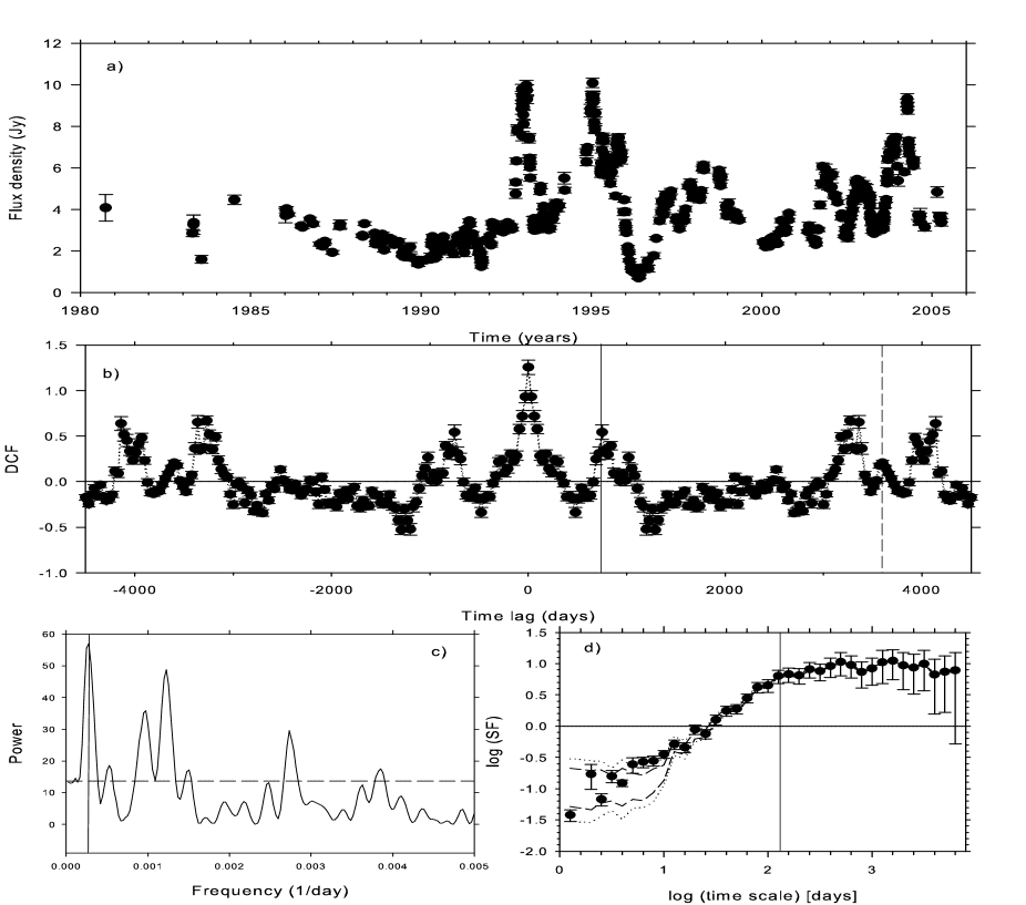
Figure 12: Analyses of the BLO source 1749+096 at 37 GHz. a) Flux Density curve. b) The discrete correlation function. The 99.5% significance level is shown with dotted line. c) The Lomb-Scargle periodogram. Dashed line shows the false-alarm probability. d) The structure function. Dashed and dotted lines show the 97.5% and 99.5% significance levels. Time scales obtained with each method are marked by vertical lines. The most significant spike of the periodogram is at time scale of 9.81 years, which is the same as the DCF correlation marked with vertical dashed line at 9.79 years time scale. The most significant DCF time scale is at 2.12 years. The SF gives a time scale of 0.34 years.

Another example, Fig. 12, showing multiple DCF correlations is a BLO source 1749+096. The most significant time scale of the DCF is at 2.12 years, but there are multiple correlations and one at the time scale of 9.79 years, corresponding to the time scale obtained with the LS–periodogram at 9.81 years. Again the SF gives a much shorter time scale of 0.34 years, which is due to the short rise times of flares at 1993 and 1995. The source has clearly changed its behaviour from the time of Paper I, where the time scale obtained is more than 10.59 years.

The results were not always this well in agreement with each other, and occasionally, it was rather difficult to find the true time scales. Usually this happens when there are gaps in the data or the flux density curve had a strong linear baseline. Mostly, however, the results were quite easily obtained and they matched well the behaviour seen visually in the flux density curves.

5.3 Intrinsic time scales and the correlations

The DCF and the periodogram give an average time of about three years between the flares. This is the time interval between the shocks in the jet. Although there were indications that BLOs and quasars may differ from each other, the differences are very small considering how different the jets in BLOs and quasars are thought to be (e.g. Aller et al. 1999).

It is also interesting to notice how little the time scale varies compared to the change in the jet parameters and luminosity. Even though the observed luminosities of these jets varied five orders of magnitude, the variability behaviour is very similar in all sources. Also, when we take the Doppler effect into account, the luminosities vary four orders of magnitude. We could expect the luminosity and the time scales to have a stronger dependence as one would expect the luminosity and the formation of the shocks to depend on the mass and the accretion rate of the central black hole. This was not seen in our analysis and it strengthens the idea that the shocks are formed by jet instabilities rather than the central engine itself. The same conclusion could be drawn from the result that the time scales are inversely proportional to luminosity meaning that greater luminosity sources have shorter time scales. One might think that in larger sources things happen more slowly and the time scales are longer as predicted by the sequence from microquasars to Low Luminosity AGNs to quasars, which gives a variability time scale that is proportional to the mass of the central black hole. Our analysis shows the opposite. Also Aller et al. (2006) found no correlation between the radio variability and the black hole mass for the MOJAVE sample.

The correlations also show that the change in time scale compared to the change in Lorentz factor is quite small. This is actually quite surprising if we think that the jet instabilities, which cause the shocks, are strongly related to the speed of the flow. Therefore in the future we need to compare the time scales with other parameters affecting the shock formation. For this we need VLBI information of a large sample of sources.

6 Conclusions

We have studied the variability time scales of a large sample of sources with different statistical methods. In our analyses we used data at frequencies from 4.8 to 230 GHz. One aim was to study how 13 more years of data affect the time scales by comparing our results with the analysis of Paper I. Many of the sources had changed their behaviour during this time and the time scales we obtained by using the structure function differed greatly from the ones in Paper I. This shows that even 10 years of monitoring is not enough to reveal the true variability behaviour of all the sources.

In many sources we could see continuous variability, for example small flares, but larger flares occur quite rarely. For some sources even 25 years is not long enough a time to reveal any characteristic time scales of variability at all.

The different methods should be used for different purposes. The LS–periodogram and the DCF give the time scale between flares and the structure function a characteristic time scale for the source, for example the rise or decay time scales of flares. When studying the correlations between the time scales and different jet parameters, we considered the DCF time scale to be the most reliable in giving the time scale between the flares. The LS–periodogram produces easily spurious spikes and therefore needs to be used with caution. In this paper also a method for studying the significance levels of the DCF was developed which in turn made the analysis more reliable.

We did not find any significant differences between the various source classes when either directly observed or redshift corrected time scales were considered. There was an indication that the BLOs may differ from quasars when intrinsic time scales are considered, but the differences are modest.

The range in time scales compared to the range of luminosities was very small indicating that the shock formation is not strongly related to the mass and the accretion rate of the central black hole but instead may be related to the jet instabilities.

1

Table 5: List of sources and frequencies. For each frequency the length of the time series and the number of observations are given.

Name		Class	22 GHz		37 GHz		90 GHz
			years	N	years	N	years	N
0007+106	III ZW 2	GAL	19.409	309	19.230	253
0016+731		LPQ	11.875	72	10.806	62
0106+013	OC 012	HPQ	22.275	197	24.155	160
0109+224	S2 0109+22	BLO	19.332	181	20.657	151
0133+476	DA 55	HPQ	22.433	335	24.165	259	14.924	73
0149+218		LPQ	15.891	147	16.687	97
0202+149	4C 15.05	HPQ	19.931	216	20.657	187
0212+735		HPQ	15.965	103	16.739	55
0224+671		LPQ	13.372	106	14.866	79
0234+285	4C 28.07	HPQ	16.172	145	15.079	105	10.260	80
0235+164		BLO	22.436	399	24.112	540	12.312	160
0248+430		LPQ	17.590	92	20.726	107
0316+413	3C 84	GAL	22.447	911	25.460	1360	14.950	265
0333+321	NRAO 140	LPQ	17.277	178	25.370	154
0336-019	CTA 026	HPQ	15.362	108	16.717	82	12.281	67
0355+508	NRAO 150	LPQ	22.428	327	25.408	268	14.950	102
0415+379	3C 111	GAL	11.504	147	12.458	88
0420-014	OA 129	HPQ	22.319	378	21.112	417	14.925	198
0422+004	OF 038	BLO	19.253	144	19.202	130
0430+052	3C 120	GAL	22.419	417	24.123	461	14.950	108
0446+112	PKS 0446+112	GAL	15.967	119	16.717	70
0458-020	PKS 0458-020	HPQ	16.163	106	17.077	86
0528+134	PKS 0528+134	LPQ	15.962	548	16.919	371	13.469	130
0552+398	DA 193	LPQ	14.045	217	14.956	171	13.406	75
0642+449	OH 471	LPQ	23.747	270	24.101	219
0716+714		BLO	15.905	203	16.742	492	8.820	84
0735+178	PKS 0735+17	BLO	23.747	309	24.038	295	14.942	99
0736+017		HPQ	21.220	208	21.902	157	11.466	79
0754+100	OI 090.4	BLO	20.329	208	25.367	170
0804+499		HPQ	15.970	257	16.744	160
0814+425		BLO	16.117	199	16.885	122
0827+243	OJ 248	LPQ	10.728	133	11.361	62
0836+710	4C 71.07	LPQ	16.060	224	16.866	226
0851+202	OJ 287	BLO	23.266	895	24.824	912	14.955	272
0906+430	3C 216	HPQ	20.318	74	21.926	53
0923+392	4C 39.25	LPQ	23.865	773	24.787	542	14.905	103
0945+408	4C 40.24	LPQ	15.819	113	16.727	55
0953+254		LPQ	15.964	156	16.706	133
0954+556	S4 0954+556	HPQ	15.816	108	16.704	55
0954+658	S4 0954+65	BLO	16.137	107	21.897	78
1055+018	OL 093	HPQ	22.430	255	24.076	229	12.744	80
1101+384	MARK 421	BLO	15.007	360	19.130	275
1147+245	B2 1147+24	BLO	15.817	63	15.792	37
1156+295	4C 29.45	HPQ	20.185	404	21.920	326	12.520	73
1219+285	ON 231	BLO	23.885	281	24.111	212
1222+216	PKS 1222+216	LPQ	10.548	243	11.320	116
1226+023	3C 273	LPQ	24.030	939	25.303	1039	14.956	352
1253-055	3C 279	HPQ	24.006	762	25.303	789	14.925	234
1308+326	AU CV n	BLO	22.283	378	24.005	315	10.043	85
1413+135		BLO	15.365	243	16.134	185	10.116	71
1418+546	OQ 530	BLO	21.051	207	21.958	182
1502+106	OR 103	HPQ	16.109	156	23.473	136
1510-089	PKS 1510-089	HPQ	19.943	245	21.926	263	14.055	111
1538+149	4C 14.60	BLO	20.327	236	21.932	181
1606+106	4C 10.45	LPQ	11.277	150	12.101	108
1611+343	DA 406	LPQ	15.964	229	16.832	198
1633+382	4C 38.41	LPQ	22.431	457	24.082	466
1637+574	OS 562	LPQ	20.175	150	21.939	156
1641+399	3C 345	HPQ	23.998	806	24.800	783	14.933	182
1652+398	MARK 501	BLO	16.111	324	16.891	218
1725+044	PKS 1725+044	LPQ	12.701	90	13.623	70
1739+522	S4 1739+52	HPQ	15.841	149	16.866	121
1741-038	PKS 1741-038	HPQ	16.027	272	16.987	295	13.351	111
1749+096	PKS 1749+096	BLO	19.858	583	24.532	465	14.099	154
1803+784	S5 1803+784	BLO	15.911	120	16.748	103	9.096	106
1807+698	3C 371.0	BLO	20.173	143	21.947	137
1823+568	4C 56.27	BLO	15.561	61	16.699	35	9.036	63
1928+738	4C 73.18	LPQ	16.055	145	16.849	101
2005+403		LPQ	22.286	318	24.032	302
2007+776	S5 2007+77	BLO	12.381	92	16.832	84
2021+614	OW 637	LPQ	16.802	107	21.932	115
2134+004	OX 057	LPQ	22.272	225	25.374	232
2136+141		LPQ	15.506	69	18.205	64
2145+067		LPQ	18.370	551	19.161	496	14.929	134
2200+420	BL Lac	BLO	24.009	965	25.443	996	14.962	145
2201+315	4C 31.63	LPQ	19.251	280	22.541	251
2223-052	3C 446	BLO	19.349	237	19.216	240	14.940	145
2230+114	CTA 102	HPQ	19.248	295	19.208	293	14.496	106
2234+282		HPQ	15.967	71	15.828	32
2251+158	3C 454.3	HPQ	24.006	760	24.480	722	14.950	244

Table 5: continued.