An approximation of the ideal scintillation detector line shape with a generalized gamma distribution
An approximation of the real line shape of a scintillation detector with a generalized gamma distribution is proposed. The approximation describes the ideal scintillation line shape better than the conventional normal distribution. Two parameters of the proposed function are uniquely defined by the first two moments of the detector response.
Joint Institute for Nuclear Research, Joliot Curie 6, 141980, Dubna Moscow region, Russia; osmirnov@jinr.ru
PACS: 29.40.Mc
1 Introduction
It is known that the response of a scintillation detector can’t be approximated by a symmetric shape since the line skewness is not zero [1] (see also discussion below). An example of the situation where the deviations of the line shape from a gaussian can lead to systematic errors is the search for the effects on the tail of beta-spectra: smearing of the spectrum due to the detector’s finite resolution provides a stronger underlying background in comparison to what one would expect in the case of a gaussian line shape.
The purpose of this work is to provide a simple analytical expression for the asymmetrical shape approximating the corresponding ideal scintillation detector response for average scintillation intensity counting from tens to hundreds of registered photoelectrons.
2 Ideal scintillation detector
The statistical properties of a scintillation detector response were studied by Breitenberg [1] and independently by Wright [2]. They showed that the relative variance of the scintillation detector pulse height is:
| (1) |
where is the relative variance of the photons transfer efficiency, is the mean signal registered at the photomultiplier (PMT) anode, measured in photoelectrons (p.e.), is the mean number of photons produced in a scintillation event and is a relative variance of the number of photons (which reduces to in the case of the normal or Poisson variance), and is a relative variance of the single photoelectron response (s.e.r.) of the photomultiplier ( and are mean position and variance of the single p.e. peak).
We will consider an ideal detector with the following features:
-
1.
anode signal for a single registered photoelectron is described by normal distribution;
-
2.
the photoelectrons are registered statistically independent;
-
3.
the number of registered photoelectrons (p.e.) for a monoenergetic source with a mean number of registered p.e. , follows a Poisson distribution, ;
-
4.
intrinsic line-width of the scintillator is negligible, the variance of the number of scintillation photons is normal;
-
5.
the detector is spatially uniform, i.e. events with the same energy produce identical responses on the average at any position inside the detector;
-
6.
noises in the system are negligible.
As it will be shown below, condition (1) is essential only when registering on the average small numbers of p.e. in an event, . Condition (2) is satisfied practically automatically in the case of detector with many PMTs working in single-electron regime, but could be questionable for a scintillator crystal coupled to a single PMT. Assumption (3) is natural, but (4) can need further validation in a real-world detector (especially in the case of the solid-state scintillators). Condition (5) is difficult to satisfy for large volume detectors, but in the case of a spatially non- uniform detector it is enough to introduce an additional parameter , defined above, to improve the fit quality. An example of fitting the 14C beta- decay spectrum in a large volume non-uniform detector will be given below (see subsection 5.3).
In [3] the case of a real scintillation detector with many PMTs is considered, and it is shown that in the above assumptions (1) reduces to:
| (2) |
where is a relative variance of the single photoelectron response averaged over all PMTs of the detector. Thus the scintillation detector consisting of many identical PMTs, surrounding the scintillator can be considered as one PMT with an extended photocathode. For this reason the terms “PMT” and the “detector” will not be distinguished in the following discussion.
If the PMT response (anode output pulse height ) to precisely photoelectrons is , and the number of the registered photoelectrons is distributed according to distribution , then the PMT response function can be written as . The PMT response function here is the probability density function (p.d.f.), it is normalized to the unity. At the absence of photoelectrons at the input of the electron multiplier () the PMT is registering the noise of the system in accordance with the p.d.f. . Using the assumption of statistical independence of the registered photoelectrons one can write the p.d.f. of registering precisely photoelectrons as a convolution of independent single-photoelectron signals . If is described with a normal distribution, then follows a normal distribution as well, with mean and variance .
With a proper choice of function the p.d.f. of the PMT response can be constructed at any mean scintillation intensity :
| (3) |
The Fourier transform of (3) gives the characteristic function:
| (4) |
where and are characteristic functions of the single photoelectron response and noise, respectively.
For the case of the Poisson distribution of the probability to register precisely p.e. in a scintillation event of mean intensity p.e., the contributions from p.e. can be summed in and (4) can be rewritten in a more compact way:
| (5) |
The analogous formula can be obtained for the generating function by using the elementary facts from the theory of branching processes [4]. In fact, omitting the noise term, equation (5) corresponds to a 2-stage cascade device: the photocathode and electrostatic focusing system providing on the average Poisson-distributed photoelectrons at the entrance of the electron multiplier with generating function ; and the electron multiplier itself with a single photoelectron response at anode with corresponding generating function . The resulting generating function has the same form as (5): , except of the noise term .
Omitting the noise term, equation (3) gets the form with characteristic function , which defines the so called compound Poisson distribution: the probability distribution of a "Poisson-distributed number" of independent identically-distributed random variables [5]. In our case the elementary distribution is the s.e.r., and the number of the independently registered photoelectrons varies in accordance with Poisson distribution (assumptions 2 and 3).
The inverse transform of (5) in some special cases of can be performed analytically, for example, the case of an exponential single photoelectron response was considered by Prescott in [6].
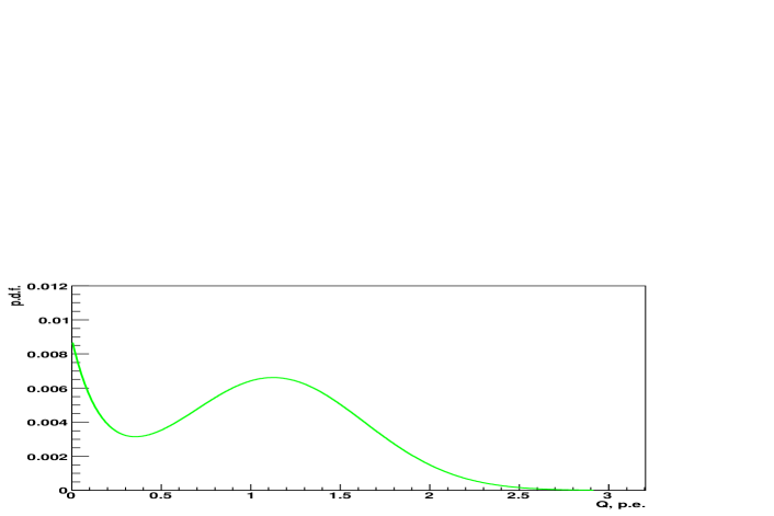
An example of realistic function is shown in Fig.1. This is the average response observed for the ETL9351 photomultiplier used in the Borexino detector [7], the measured mean relative variance over a set of 2200 PMTs selected for the detector is [8]. If the single photoelectron response of PMT and noise function are known, then formula (5) can be used to construct the PMT response for any for which the basic assumptions are valid. The method based on the use of transform (5) has been successfully applied to fit the experimental spectra obtained with electrostatically focused hybrid photomultiplier tubes for few registered photoelectrons ( and p.e.) in [9], where formula (5) was called "light spectra sum rule".
It should be noted that single photoelectron spectra of the photomultiplier studied in [9] has a very narrow single p.e. peak, so that the detector response to has "fine structure” peaks around the values corresponding to integer numbers of the registered charge. In this article we consider a case of with big enough to make the contribution of the first resolved fold photoelectron peaks to be negligibly small. The parameter can be obtained from the following considerations. The PMT response to precisely p.e. (n-fold peak) with increase of converges very fast to a normal distribution with and as it follows from the central limit theorem. In practice the PMT response to as low as p.e. can be approximated by a gaussian, see i.e. [10]. The (n-1)-fold and n-fold peaks are not resolved if the half width on the half heights resolution of the n-th peak is worse than : , i.e. . The contribution of responses from few photoelectrons decreases very fast with the increase of . It is easy to check that the condition is satisfied already at p.e. In this case instead of the real shape of the PMT single electron response one can choose the gaussian approximation for the function , with mean and variance coinciding with the corresponding parameters of the real-shape function. Indeed, the response functions for 3 and more p.e. are well approximated by a normal distribution, and 0,1 and 2 photoelectrons contribute less than 1% to the total spectrum (see also Fig.2).
In such a way an ideal detector response is described by the inverse transform of (5) with corresponding to the characteristic function of a gaussian with the mean value and variance of the corresponding single photoelectron response:
| (6) |
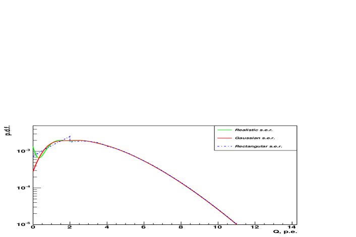
In the following discussion we call the "ideal" detector response obtained from (5) by using from (6), and we let the "real" detector response to refer to (5) with obtained by transforming the real shape of the single photoelectron response. The difference between the "real" and "ideal" scintillation response vanishes very fast with the increase of (at p.e.). We have chosen the gaussian shape for s.e.r. for convenience, but any appropriate s.e.r. line shape can be used (with a relative variance that of real s.e.r.). This is illustrated in Fig.2, where the theoretical photomultiplier responses for p.e. obtained for 3 different s.e.r. function (realistic from Fig.1, gaussian and rectangular) with the same mean value and variance, are plotted. One can see that the difference is noticeable only at the registered charge p.e., the tail of the PMT response is modeled equally good with the gaussian and rectangular s.e.r. functions111So, attempts to evaluate the single electron response spectrum at seems to be senseless for the PMT spectra with unresolved s.e.r. (), in the best case one can succeed to extract and values, but not the details of the s.e.r. shape..
3 The normal distribution as a limit case for ideal scintillation detector response
The ideal detector response converges quickly to the normal distribution as grows. In fact, the Poisson distribution of the primary photoelectrons at the input of the electron multiplier converges to a normal distribution for big . The variance in the multiplication of the photoelectrons arriving at the electron multiplier, for high values can be considered roughly the same for all possible values of the registered number of photoelectrons (). So, in the big limit the ideal response converges to the convolution of two gaussian processes which give a normal distribution with the mean value and variance, respectively:
| (7) |
coinciding with the values found above considering statistical properties of the scintillation registration process. We assume that the scale is calibrated in photoelectrons, i.e. (otherwise it is necessary to pass to variable ). The characteristic function for a gaussian p.d.f. is:
| (8) |
and it is apparently different from an ideal shape characteristic function (5) with from (6). Moreover, one can calculate the moments of the ideal scintillator response from its generating function:
| (9) |
and check that only the first two moments of the gaussian and ideal responses are equal. The third central moment calculated for the ideal response is which neither coincides with that of a normal distribution (it is simply zero), nor converges to it with increasing . Only the skew , which is a measure of the distribution asymmetry, indeed converges to zero slowly enough as .
Although the normal approximation of the scintillation line shape is quite common [1], there are situations in which its use leads to systematic errors in the parameter definition. Two examples will be considered below (see section 5). In order to resolve this problem, a better approximation of an ideal scintillation shape is needed.
4 The generalized gamma distribution as a limiting case for the ideal response
We will search for a function with the following properties:
-
1.
the function converges to a normal distribution for ;
-
2.
it has the mean value and variance coinciding with that of the ideal scintillator response;
-
3.
it approximates the ideal scintillator response better than a conventional normal distribution;
-
4.
it is asymmetric with a skew decreasing as , and gives a better approximation of the distribution tail.
In literature the successful usage of the 2-parameter gamma- distribution to approximate the output pulse height spectra of scintillation detectors is reported, with better results in comparison with a normal approximation [11],[12]. We were not able to get a good agreement with the response function of an ideal detector using the above- mentioned distribution, so we have chosen a power transformed gamma distribution (also known as generalized gamma distribution) as a candidate:
| (10) |
The distribution describes a variety of well-known 1 and 2-parameter probability laws as special cases; more details regarding the distribution properties can be found in [13]. A physical basis for the generalized gamma distribution has been discussed by Lienhard and Meyer in [14].
We start by fitting the ideal scintillator response for different values using (10) with 3 free parameters. It has been discovered that over a wide region of the value of parameter is close to 2, thus we fix it at this value and use the following distribution as an approximation of the ideal shape response (redefining from (10) as ):
| (11) |
with parameters and providing equality of the mean value and variance of (11) to the corresponding values of the ideal scintillation response. It is easy to check that the moment of order of the distribution (11) is:
The parameters and can be defined from the system of equations:
| (12) |
A recipe for the approximate solution of the system is given in Appendix A. An alternative way of calculating the parameters and based on the equality of the first two even moments of (11) to the corresponding values of the ideal scintillation response, is presented in Appendix B.
It is important to stress that a special case is found in many physical applications: in hydrology it is known either as hydrograh distribution [14], or in countries where the Russian hydrology school has become more familiar, as the Kritskiy- Menkel distribution [15]; in radio-engineering variants of the generalized gamma-distribution are widely used to describe radio waves propagation in fading environment (Nakagami distribution [16]); some further examples can be found in [17]222In [13] the case is called Stratonovich distribution. We were unable to find the corresponding reference in literature..
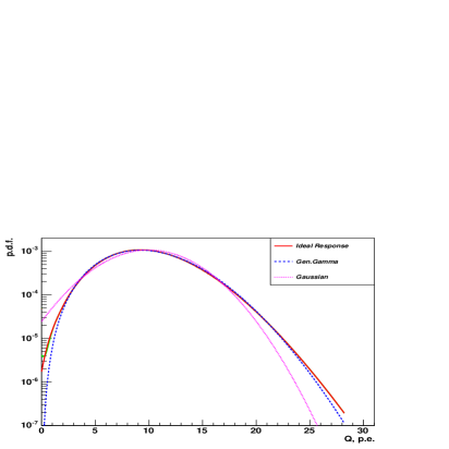
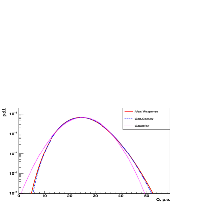
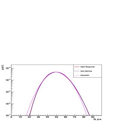
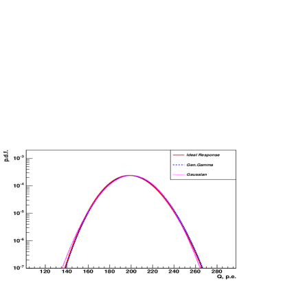
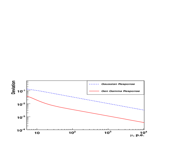
In the limit the distribution converges to a normal distribution [18], the condition 2 is satisfied automatically, conditions 3 and 4 have been checked numerically in a wide range of values. As it can be seen in Fig.3 the generalized gamma distribution approximates the ideal response better than a gaussian. Fig.4 presents results of numerical calculations of the deviation of the gaussian (with the mean value and variance that of an ideal response) and the shape obtained with (11) from the ideal response calculated as:
| (13) |
and has a simple mathematical interpretation. In Fig.4 one can see that the deviation of the generalized gamma-distribution from the ideal one calculated by using (13) is an order of magnitude lower than that in the gaussian distribution case.
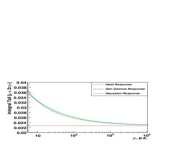
The quality of the fit in the tail has been checked by calculating the integral in the region for the ideal and generalized gamma- distributions. The integral of the gaussian in this region is constant defined by the complementary errors function: . The cumulative distribution corresponding to the density (11) is:
| (14) |
where is the normalized incomplete gamma function. The integral in the tail is .
Integral in the tail for the ideal response was calculated by using the original definition (3):
with and . The results are presented in Fig.5. One can see that the gamma distribution gives a better approximation of the distribution tail than the gaussian one.
5 Two examples
The precision of the description of the spectra of a real scintillation detector with respect to different approximations of the response function has been verified by using both the real data of the Counting Test Facility (CTF, [19]) of the Borexino detector [7], and the data obtained with the Monte Carlo model of the CTF detector. In the present article we consider only the MC data, the results of comparison of the theoretical model with the real CTF data will be presented by the Borexino collaboration.
The large volume liquid scintillator detector CTF is a prototype of the solar neutrino detector Borexino. The CTF was used to develop the methods of deep purification of the liquid scintillator and water from the natural radioactive impurities. The CTF consists of 3.7 tones of liquid scintillator on the base of pseudocumene (C9H12), contained in a transparent spherical inner vessel with a radius of 1 m, and viewed by 100 photomultipliers (PMTs) mounted on an open spherical steel support structure. The PMTs are equipped with light concentrator cones to increase the light collection efficiency; the total geometrical coverage of the system is . The radius of the sphere passing through the opening of the light cones is 2.73 m. The entire detector is placed inside a cylindrical tank with water, which provides shielding against external gammas. On the bottom of the tank another 16 PMTs are mounted to identify cosmic muons by their Cherenkov light produced in the water. The detailed description of the CTF detector can be found in [19]. The CTF has been in operation since 1993. At present it is in its third data-taking campaign (CTF3) with the main goal of tuning the purification strategy for the Borexino detector. The data collected with an upgraded version of the CTF were used by Borexino collaboration in order to search for a number of possible manifestations of non-standard physics, a review of experimental results can be found in [20].
The Monte Carlo model of the CTF detector was developed on the basis of EGS-4 code [21] to check the validity of the background interpretation. It accounts for the dependence of the light yield on the energy (ionization quenching) and on the position where energy was deposited inside the detector. The model has been calibrated with the CTF data and describes the CTF experimental spectra with a satisfactory precision. For the purposes of the present work, the model of the detector response was changed to take into account the deviations of the response function from the normal one (the standard program uses the normal approximation of the response function).
5.1 Monoenergetic line
The detector response to the monoenergetic particle has been modeled with the MC method. The particle energy was chosen in order to provide the number of registered photoelectrons, p.e. The number is big enough to ensure good approximation with a gaussian shape. Indeed, the processing of the CTF data by using this approximation was successfully applied even for lower values of the mean registered charge [22].
The response of the detector was generated in the following way. First, the mean number of p.e. registered at one PMT was defined as , where is the total number of the PMTs in the detector. Then in each event for each PMT the Poisson- distributed number of registered p.e. was generated, and, finally, the registered anode charge was simulated using the gaussian approximation of the PMT signal with mean and variance . The response of the detector is the sum of signals over all PMTs of the detector. events were simulated.
The MC data were fit with the gaussian response function and with the response function based on the generalized gamma- distribution. The results of the fit are presented in Table 1 and Fig.6. The mean values and the normalization are reproduced well for the gaussian and generalized gamma line shapes; the difference in variances is within the statistical precision of the method. The value for the gaussian case excludes the hypothesis of the normal line shape; in the case of the non-gaussian shape we have a good match of the data with the model (, the number of degrees of freedom (n.d.f.) here is the number of bins used in the fit with the number of free parameters subtracted). We have found no difference when applying method A or B (see Appendix A and B) to estimate of parameters of the non-gaussian line shape.
As it is noted above, Prescott in [6] obtained a precise line shape for the case of an exponential single photoelectron response , , it reads:
| (15) |
where is a modified Bessel function of the first kind for an imaginary argument.
The slope of an exponential distribution coincides with its mean value, i.e. . The variance of the single electron exponential response doesn’t depend on parameter and is . It is clear that formula (15) can’t be directly applied to fit the real scintillation shape. The way to solve this problem was pointed out in [6]: it is enough to treat as a scale parameter, the variance in this case will scale as and the mean value as . In order to preserve the mean value and variance in the original scale, we multiply by a scale parameter , and as before set :
| (16) |
Now formula (16) can be used to fit the scintillation line, the results are presented in Table 1. Comparing the values one can see that the quality of the fit with Prescott formula is worse than in the case of the fit with the generalized gamma function, but much better than in the case of the fit with the normal distribution. The quantitative comparison of the models can be performed using Fischer’s F-distribution as a significance test: , where is a number of the degrees of freedom and is a confidence level [23]. Solving equation with respect to one can exclude the gaussian shape with a c.l. more than 99.99. The scintillation line shape is described better by Prescott’s formula (as can be seen from the comparison of values in Table 1) and the exclusion c.l. is smaller, but Prescott’s model fails to describe the data with high precision as the generalized gaussian distribution does.
The obtained results have demonstrated very weak sensitivity of the real line shape to the shape of the s.e.r., so one can choose any convenient s.e.r. shape in order to invert formula (5).
| Norm () | ||||
|---|---|---|---|---|
| MC input | 150.00 | 14.18 | 1.000 | |
| Gauss | 150.010.05 | 14.190.03 | 1.0000.001 | 1883/116 |
| Gen.gamma | 150.020.05 | 14.170.03 | 1.0000.001 | 111.6/116 |
| Prescott | 149.520.05 | 14.190.03 | 1.0000.001 | 329.0/116 |

5.2 beta spectrum: MC model of the experimental data
The major part of the background in the ultra-pure CTF in the energy region up to 200 keV is induced by -activity of [24], which is present in the organic liquid scintillator at the level of g/g. The -decay of is an allowed ground-state to ground-state () Gamow-Teller transition with an endpoint energy of keV and half life of 5730 years. The end-point of the decay is used in CTF to establish the energy scale, thus the precision of the modeling of 14C spectrum defines the precision of the energy scale calibration.
The beta energy spectrum with a massless neutrino can be written in the following form [25]:
| (17) |
where
and are the total electron energy and momentum;
is the Fermi function with correction of screening caused by atomic electrons;
contains departures from the allowed shape.
For we have used the function from [26] which agrees with tabulated values of the relativistic calculation [27]. A screening correction has been made by Rose’s method [28] with screening potential eV. The spectrum shape factor can be parametrized as (see [29] for more details), the value of the parameter was fixed at the value MeV-1.
The deviations of the light yield from the linear law have been taken into account by using the ionization deficit function , where is Birks’ constant [30]. To calculate the ionization quenching effect for the scintillator on the base of pseudocumene, we used the KB program from the CPC library [31]. The value of the ionization quenching parameter cm-1MeV-1 was fixed at the value found by independent experiments. The radial dependence of the mean registered charge on the point of interaction inside the detector has been accounted for with the function, obtained from the experimental data (see [3]). For convenience the value of the function at the detector’s center was assumed to be the unity, .
The response of the detector for an event of 14C decay was generated in the following way. First, the event energy was generated according to the spectrum (17), and the position of the event was generated in assumption of uniform distribution of 14C decay events in the detector volume. Then the mean number of p.e. has been defined, registered for an event of energy occurring at distance from the detector center, taking into account detector’s non-uniformity and non- proportionality of the light yield on the energy:
where is the scintillator specific light yield measured in photoelectrons per MeV.
Then in each event for each PMT the mean value of registered number of p.e. has been defined, and the registered p.e. number was generated according to the corresponding Poisson distribution. Finally, the registered anode charge was simulated by using a gaussian approximation of the PMT signal with mean and variance . The response of the detector is the sum of the signals over all PMTs of the detector. event were simulated, that corresponds approximately to 3 years of continuous data taking with the CTF detector.
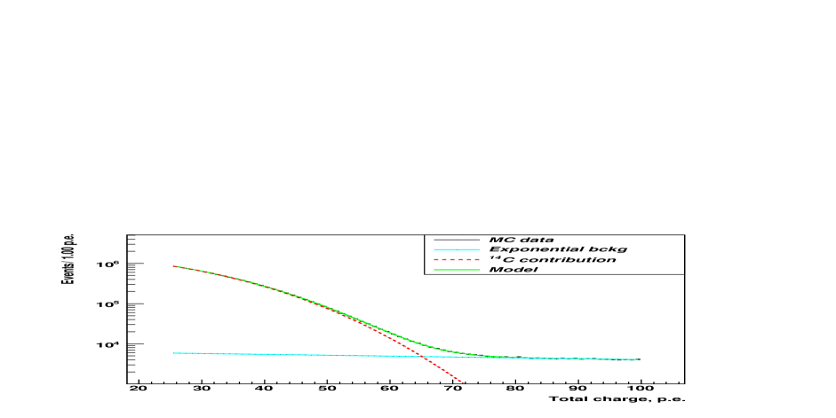
The exponential underlying background has been added to the 14C -spectrum to simulate the realistic situation. We have taken the parameters of the exponential observed in the CTF detector. This background is mainly due to the external ’s from decays of elements from 238U and 232Th chains in the water shield.
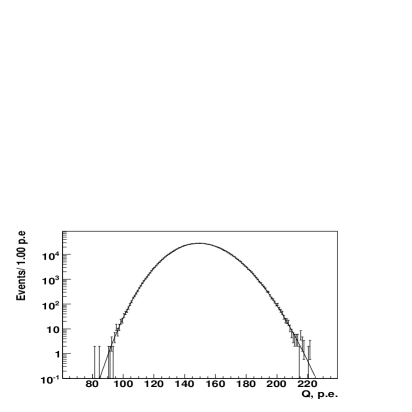
5.3 beta spectrum: fitting MC data with model function
The real detector response to uniformly distributed events is not spatially uniform. To take into account the additional pulse height variance we exploit formula [3]:
| (18) |
where
-
is the mean total registered charge for the events of the energy E uniformly distributed over the detector volume. is the mean value of the function over the detector volume;
-
is the relative variance of the PMT single photoelectron charge spectrum () averaged over all PMTs of the detector ( in total) taking into account the i-th PMT relative sensitivity . For the CTF detector this parameter has been defined with a high precision during acceptance tests [8] and turns out to be ;
-
is the scintillator specific light yield measured in photoelectrons per MeV;
-
is the relative variance of the photon transfer efficiency, mainly due to the spatial non-uniformity of the detector. Among other additional contributions there is the intrinsic scintillator line width, the precision of the detector calibration, the precision of zero signal definition, etc. There is now need to keep these additive parameters apart, so in the model we have left the only parameter. In the MC modeling these additional contributions were set to zero, but, nevertheless, parameter remained free, see discussion below.
The MC spectrum was modeled with a sum of two components: (1) convolution of the beta spectrum with the detector resolution function with 3 free parameters: total normalization , light yield , and additional variance ; (2) an additional exponential background with 2 free parameters.
The final model function has 5 free parameters and is presented as:
| (19) |
where is the detector response function, and N(E) is the beta- spectrum (17).
| Norm () | Slope | |||
|---|---|---|---|---|
| MC input | 391.8 | 5.000 | 100.0 | |
| Gauss | 387.80.3 (-13) | 5.1740.010 (+17) | 99.20.5 () | 279.7/214 |
| Gen.Gamma | 394.00.3 (+7 ) | 5.0330.008 (+4) | 100.00.3 (0) | 211.3/214 |
The results of the fit of the experimental data with the gaussian and non-gaussian line shapes in 30-250 p.e. region, are presented in Table 2. Again, the is much better for the non-gaussian line shape. The comparison of the models excludes the gaussian shape on the c.l. of 98 (solution of with gives ).
This time relatively big deviations in parameters have been found when applying different resolution functions. The deviations for parameters are bigger than statistically allowed, so it should be treated as systematic errors. As it follows from Table 2, the error in the light yield definition for the case of the gaussian line shape is , the error of the total normalization is . With the generalized gamma function the error in light yield is smaller: , the same error has the total normalization.
It is not implicitly assumed that additional broadening of the scintillation line shape () is distributed in the same way as the main contribution . The statement is not true in general, especially for big values where term can dominate in the response. In our case the main term dominates, that is confirmed by the quality of the fit, so the precise distribution for the additional line broadening can be neglected. The price paid for this simplification is the observed systematical deviations.
When fitting the monoenergetic line from decays of 214Po without selecting the detector central region the quality of the fit is much worse at the left side of the peak. In the case of 14C spectrum these imperfections on the left side are covered due to the fast decrease in the spectrum and the gaussian shape is justified. On the right side the proper description of the scintillation line tail is important because of the same fact of the fast decrease of the spectrum. In the case of the monoenergetic line the true shape of the distribution of the mean values over the detector volume, has to be taken into account.
6 Conclusions
An approximation of the real line shape of the scintillation detector with the generalized gamma distribution has been proposed. The approximation describes the ideal scintillation line shape better than the widely used normal distribution. Two parameters of the proposed function are uniquely defined by the first two moments of the detector response or by the first two even moments. The computational complexity of the resolution function calculation is comparable to that of the normal resolution.
It has been demonstrated that the ideal detector response to many photoelectrons () loose the sensitivity to the shape of the single electron response of a photomultiplier and the only important parameter is the s.e.r. relative variance. In analytical calculations any convenient function can be used instead of a real s.e.r.
While for the relatively "flat" experimental spectra one can hardly expect the enhancement of the overall quality of the fit, in the case of the fast-varying distributions, such as tails of the spectrum, the use of the proposed resolution function allows one to exclude the artifacts associated with resolution mismatch, and avoid systematics errors as demonstrated by the example with the 14C spectrum fit.
Acknowledgments
I am very grateful to Ferenc Dalnoki-Veress and Svetlana Chubakova for the careful reading of the manuscript and useful discussions.
Appendix A
| (20) |
For big the expansion converges fast because of . Taking three first terms and substituting in the first equation, we obtain a simple quadratic equation
with the only positive root:
| (21) |
which gives the solution with a relative precision of for . A more accurate solution can be obtained by using more terms from the expansion (20). Assuming that more accurate solution has a form and developing and two remaining terms from (20) into a Tailor series keeping only a linear term with respect to , we obtain a linear equation for with the following solution:
| (22) |
Equation (22) gives the relative precision of the parameter estimation of at , at it is .
Appendix B
In radio-engineering the generalized gamma-distribution variant are widely used to describe radio waves propagation in fading environment. One of the most popular is the m-distribution proposed by Nakagami [16] in the functional form
where , and is the inverse of the relative variance of . The advantages of this equation are simple rules to calculate the parameters.
In fact, for the even moments of (11) the system of two equations for and will not contain gamma- functions. Using the parameters and we can write the second and the fourth moments:
| (23) |
The solution of this system is
| (24) |
In order to use (24), we should require the equivalence of the first two even moments of (11) to those of the ideal scintillator response, which can be easily calculated with (9):
References
- [1] Breitenberger E., Scintillation spectrometer statistics, in Progr. in Nucl.Phys. 1955. V. 4. P. 56.
- [2] Wright G.T. J.Sci.Instrum. 1954. V. 31. P. 377.
- [3] Smirnov O.Ju. Instr. and Exp. Technique 2003. V. 46. P. 327.
- [4] Sevastianov B. A. Branching processes. Moscow. Nauka. 1971.
- [5] Feller W. “An introduction to probability theory and its applications”, vol.1-2, Wiley, 1967.
- [6] Prescott J.R. Nucl.Instrum.Methods. 1963. V. 22. P.256.
- [7] The Borexino Collaboration, Alimonti G., Arpesella C., Back H. et al. Astroparticle Physics. 2002. V. 16. P. 205.
- [8] Ianni A., Lombardi P., Ranucci G., Smirnov O. Ju. Nucl.Instrum.Methods Phys.Res. Sect. A. 2005. V. 537. P. 683.
- [9] de Fatis T.T. Nucl.Instrum.Methods Phys.Res. Sect. A. 1997. V. 385. P. 366.
- [10] Dossi R., Ianni A., Ranucci G., Smirnov O. Ju. Nucl.Instrum.Methods Phys.Res. Sect. A. 2000. V. 451. P. 623.
- [11] Gale H.J. and Gibson J.A.B. J.Sci.Instrum. 1966. V. 43. P. 224.
- [12] Stokey R. J. and Lee P. J. The Telecommunications and Data Acquisition Progress Report 42-73, January-March 1983, Jet Propulsion Laboratory, Pasadena, California. 1983, May 15. P. 36; http://tmo.jpl.nasa.gov/tmo/progress report/42-73/73D.PDF
- [13] Hegyi S. Phys. Lett. B. 1996. V. 387. P. 642.
- [14] Lienhard J.B. and Meyer P.L. Quarterly of Applied Mathematics, 1969, Vol.XXV, No.3.
- [15] Kritskiy S.N. and Menkel M.F., Izv.Akad.Nauk SSSR (Otd. Techn. Nauk) No.2, Moscow, 1946.
- [16] Nakagami M., The m-distribution-A general formula of intensity distribution of rapid fading, in Statistical Methods in Radio Wave Propagation, Pergamon Press, Oxford, UK. 1960. P. 3.
- [17] Schenzle A. and Brand H. Phys.Rev. A 1979. V. 20. P. 1628.
- [18] Haken H., Synergetics, An Introduction. Springer Verlag. Berlin. 1977.
- [19] The Borexino Collaboration, Alimonti G., Arpesella C., Bacchiochi G. et al. Nucl. Instrum. and Methods. Sect. A. 1998. V. 406. P. 411.
- [20] Derbin A.V., Smirnov O.Yu., and O.A.Zaimidoroga Physics of Particles and Nuclei. 2005. V. 36. No. 3. P. 314.
- [21] Nelson W.R., Hirayama H., Rogers D.W.O. The EGS4 code system. SLAC-265. 1985.
- [22] The Borexino Collaboration, Back H.O., Balata M., de Bari A. et al. Phys.Letters B. 2003. V. 35. P. 563.
- [23] Wolberg J., Data Analysis Using the Method of Least Squares, Springer-Verlag, Berlin Heidelberg, 2006.
- [24] The Borexino Collaboration, Alimonti G., Angloher G., Arpesella C. et al. Phys.Lett. B. 1998. V. 422. P. 349.
- [25] Morita M., Beta Decay and Muon Capture. Benjamin, Reading, Mass. 1973. P. 33.
- [26] Simpson J.J., Hime A. Phys.Rev. D. 1989. V. 39. P. 1825.
- [27] Behrens H., Janecke J., Numerical Tables for beta-decay and electron capture. ed. H.Schopper, Landolt-Bornstein. Springer. Berlin. 1969.
- [28] Rose M.E. Phys.Rev. 1936. V. 49. P. 727.
- [29] Kuzminov V.V., Osetrova N.Ia. Physics of Atomic Nuclei. 2000. V.63. No. 7. P. 1292.
- [30] Birks J.B., The Theory and Practice of Scintillation Counting, New York: Macmillan, 1964.
- [31] Los Arcos J.M., Ortiz F. Comput. Phys. Commun. 1997. V.103. P. 83.
- [32] Graham R. L., Knuth D. E. and Patashnik O. Answer to Problem 9.60 in Concrete Mathematics: A Foundation for Computer Science, 2nd ed. Reading, MA: Addison-Wesley, 1994.