Spreading gossip in social networks

Abstract

We study a simple model of information propagation in social networks, where two quantities are introduced: the spread factor, which measures the average maximal fraction of neighbors of a given node that interchange information among each other, and the spreading time needed for the information to reach such fraction of nodes. When the information refers to a particular node at which both quantities are measured, the model can be taken as a model for gossip propagation. In this context, we apply the model to real empirical networks of social acquaintances and compare the underlying spreading dynamics with different types of scale-free and small-world networks. We find that the number of friendship connections strongly influences the probability of being gossiped. Finally, we discuss how the spread factor is able to be applied to other situations.

I Introduction and model

In every-days life probably everyone has already experienced the annoying situation of telling some personal secret to some friend and ending with a naive “please, do not tell that to anyone, ok?” and after short time all our friends suddenly know the secret. What happened? Is this common phenomenon a consequence of a natural instinct that friends have to conspire and slander against each other? Or is this a phenomenon which can hardly be avoid by human trust and respect being closely related to the net of acquaintances that people naturally tend to form?

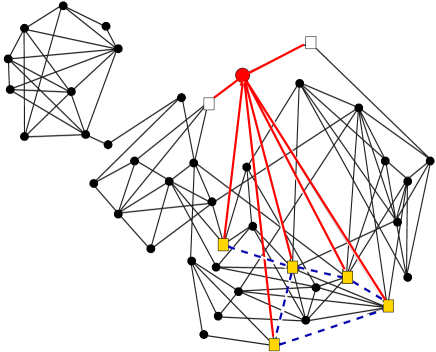
Figure 1: (Color online) Spreading of information about a target-node shown as the grey (red) open circle on part of a real school friendship network schools . If the spreading starts from one of the white squared neighbors, no propagation occurs ($f=0$). If instead, one of the grey (yellow) squared neighbors starts the spreading, in $\tau=3$ time-steps, five neighbors will know it, giving $f=5/7$. The information spreads over the dashed (blue) lines. The information can be seen as a gossip about the target-node or the victim (see text). Note that the clustering coefficient of the victim has a different value, namely $C=10/42$.

Such kind of questions can be easily addressed by representing the social system, composed by individuals and the interactions among them, as a network, i.e., as a collection of nodes and links. While networks have been widely used by physicists to study e.g. porous media hans05 or a system of interacting spins sanchez02 ; krapivsky03 ; mobilia03 , they can also be used to study social systems. Social networks have helped to further understand the structure and evolution of social systems, where people and their acquaintances are represented by the nodes and links of the network respectively. In particular, propagation of information in social systems is easily reproduced in such networks and has been addressed in recent physical literature boccaletti05 ; shao03 ; cycles due to its importance in epidemiology dodds04 , where information is related to the contagious of diseases, to understand social influence, beliefs and extremism castellano00 ; pluchino05 ; galam05 ; he04 , to understand the evolution of financial markets eguiluz00 , to study econophysical networks underlying e.g., electrical supply systems or road webs among airports or cities. Here we put emphasizes on how far the information can spread when particular constraints, of interest for social systems, are taken into account.

The way information spreads over the network depends on its content. A rumour or an opinion concerning some topic which is not directly connected to the social network structure (political opinion, etc) can be of interest to any of the neighbors of a certain node, regardless their topological features. However, as opposed to rumors, a gossip always targets the details about the behavior or private life of a specific person, i.e., of a specific node. This node will be called henceforth the target-node or the victim. Therefore, due to this particular content, it is reasonable to assume as a first approach that the information spreads only over people directly connected to the victim.

A simple model recently introduced us for such kind of information spreading is described as follows. Selecting randomly a victim, the gossip about him or her is created at time $t=0$ by an originator which shares a bond with the victim. At $t=1$ the originator only spreads the gossip to other nodes, which are connected to him-/herself and the victim. The spread continues until all reachable acquaintances of the victim know it, as illustrated by the squares connected by dashed lines in Fig. 1 for a real friendship network schools . Our dynamics is therefore like a burning algorithm burning , starting at the originator but limited to sites that are neighbors of the victim.

To measure how effectively the gossip - or, in general, the information - attains the acquaintances of the victim, we define the spreading factor as $f=n_{f}/k$, where $n_{f}$ is the total number of people who eventually hear the gossip and $k$ is the degree of the the victim. In addition, we also define the spreading time $\tau$ which defines the minimum time it takes to reach this fraction $f$ of acquaintances, giving a measure of how far these connected acquaintances are from each other. It is important to note that $f$ and the standard definition of clustering coefficient $C$ watts98 ; Amaral00 are different quantities, since the later only measures the number of bonds between neighbors and contains no information about how such bonds distribute among the victim’s acquaintances.

We start in Sec. II by studying how such kind of information spreads in different networks, namely in scale-free and in small-world networks. Some analytical considerations will be present for the particular case of the Apollonian network hans05 . The results of such artificial networks are also compared to the ones obtained with an empirical network of social contacts recently obtained from an U.S. School survey schools , where friendship acquaintances were rigorously defined schools ; prl . There are also situations where the information about the target-node can be of interest beyond the first neighbors, like the case where the victim is a movie star, yielding a scenario similar to the one of usual rumour propagation or even epidemic spreading telogama . These cases will be considered in Sec. III. Since the tendency for spreading information does not always implies that its transmission will be certain, we introduce in Sec. IV a probability for each node to spread the information and study the main effects on the spreading dynamics. Discussion and conclusions are given in Sec. V.

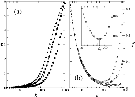
Figure 2: (a) Spreading time $\tau$ in a Barabási-Albert scale-free network and (b) the spreading factor $f$, both as a function of $k$: $m=3$ (circles), $m=5$ (squares) and $m=7$ (triangles). The dashed line in (b) indicates $f=1/k$. The inset in (b) is a zoom of the plot for $m=5$ emphasizing the optimal degree $k_{0}$ which minimizes the gossip spreading (see text). In all cases, $N=10^{4}$ nodes, averages over $500$ realizations are considered, and logarithmic binning in $k$ is used.

II Spreading information over first neighbors

We consider first a Barabási-Albert (BA) scale-free network barabasi99 : starting with a small number $m$ of nodes fully connected to each other one adds iteratively one new node with $m$ initial links attached to the nodes of the network with a probability proportional to the node degree.

In Fig. 2a we show the average spreading time $\tau$ as a function of the degree $k$ in a scale-free network with $N=10^{4}$ nodes and $m=3,5$ and $7$. In all cases, for large values of $k$, $\tau$ scales logarithmically with the degree

$$\tau=A+B\log{k}$$ (1)

where for this case $A=-10.77$ and $B=2.433$ defines the dashed line in Fig. 2a.

For the same values of $m$ we plot in Fig. 2b the dependence of the spread factor with the degree. Curiously, one sees an optimal degree $k_{0}$ for which the spreading factor attains a minimum (see inset). This optimal value lies typically in the middle range of the degree spectrum showing that the two extreme situations of having either few or many neighbors enhance the relative broadness of the information spreading. Further, a closer look shows that for small degrees the values of $f$ coincide with $f=1/k$ (dashed line) while for larger degrees $f$ deviates from $1/k$ with a deviation which increases with $m$. Thus, while initially ($t=0$) the spread factor is always $f=1/k$ (dashed line), for the subsequent time-steps one observes that nodes with small degrees remain on average at $f=1/k$ while for large degrees the spread factor increases up to a maximal value.

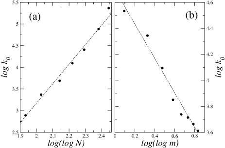
Figure 3: The optimal degree $k_{0}$ in a BA network as a function (a) of $N$ fixing $m=5$ initial outgoing connections and (b) of $m$ for $N=10^{4}$ nodes. The average degree is $\langle k\rangle=2m$. The dotted lines have slopes of $a=4.64$ and $-b=-1.34$ (see Eq. (2)).

The dependence of the optimal value $k_{0}$ on the two parameters $N$ and $m$ is studied in Fig. 3. Here, we observe that the optimal degree $k_{0}$ yields approximately

$$k_{0}\propto\frac{(\log{N})^{a}}{(\log{m})^{b}}.$$ (2)

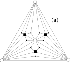
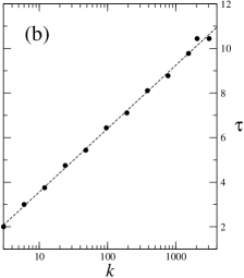
Figure 4: (a) Illustration of the first three generations of an Apollonian network (see text). (b) Spreading time $\tau$ for the spreading factor to attain the maximal value $f=1$ where the dashed line can be obtained analytically (see text) yielding an expression as in Eq. (1) with $A=-0.28$ and $B=1.1$.

The scale-free networks considered above are probabilistic. In other contexts, deterministic scale-free networks have been proposed hans05 ; dorogpseudo , as a way to construct perfect hierarchical networks. One of such networks is the Apollonian network. The Apollonian network is constructed in a purely deterministic way hans05 ; pre04 as illustrated in Fig. 4a: one starts with three interconnected nodes, defining a triangle; at $n=0$ (generation $0$) one inserts a new node at the center of the triangle and joins it to the three other nodes (white circles in Fig. 4a), thus defining three new smaller triangles; at iteration $n=1$ one adds at the center of each of these three triangles a new node (squares), connected to the three vertices of the triangle, defining nine new triangles and then for generation $n=2$ one node (black circles) at the center of each of these nine triangles and henceforth. The number of nodes and the number of connections are given respectively by $N_{n}=\tfrac{1}{2}(3^{n+1}+5)$ and $L_{n}=\tfrac{3}{2}(3^{n+1}+1)$. The distribution of connections obeys a power-law, since the number of nodes with degree $k=3,3\cdot 2,3\cdot 2^{2},\dots,3\cdot 2^{n-1},3\cdot 2^{n}$ and $2^{n+1}$ is equal to $3^{n},3^{n-1},3^{n-2},\dots,3^{2},3,1$ and $3$, respectively. Thus one has $P(k)\propto k^{-\gamma}$ with $\gamma=\ln{3}/\ln{2}$.

One main difference from the BA network is that, for Apollonian networks $f=1$ independently of $k$, due to the hierarchical structure shown in Fig. 4a. In Fig.4b one observes the logarithmic behavior of $\tau$ similar to the BA case. In the Apollonian case the logarithmic behavior can even be derived analytically as follows. From Fig. 4a one sees that vertices belonging to the $n$th generation communicate with each other through $n$ steps thus $\tau\propto n$. Since the degree of the $n$th generation is given by hans05 $k=3\times 2^{n-1}$, one obtains the logarithmic dependence of $\tau$ shown in Fig. 4c, where the dashed line yields the expression in Eq. (1) with $A=-0.28$ and $B=1.1$.

Next, we show that the main results obtained for the scale-free networks above are also characteristic of real empirical social networks. For that, we study the model for information propagation on a real social network, namely, the one extracted from empirical data obtained in an extensive study done within the National Longitudinal Study of Adolescent Health (AddHealth) schools at the Carolina Population Center. The data comprehends a survey done between 1994 and 1995 in $84$ American schools evaluating an in-school questionnaire to $90118$ students. The students are separated by the school they belong to and therefore there are $84$ networks with sizes ranging from $\sim 100$ to $\sim 2000$ students. The aim is to allow social network researchers interested in general structural properties of friendship networks to study the structural and topological properties of social networks bearman04 . In previous studies prl ; physicaD , it has been shown that the main properties characterizing the underlying networks from these data can be easily reproduced with a mobile agent model.

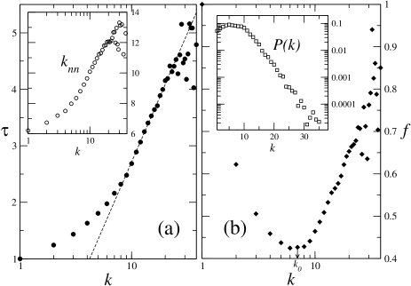
Figure 5: Propagation of information on a real friendship network of American students schools averaged over 84 schools. In (a) we show the spreading time $\tau$ as function of degree $k$, plotting in the inset, the average degree $k_{nn}$ of neighbors of nodes with degree $k$. In (b) the spread factor $f$, both as a function of degree $k$, with the inset showing the degree distribution $P(k)$.

As shown in Fig. 5a, while for small $k$ the spreading time grows linearly, for large $k$ it follows a logarithmic law given by Eq. (1) with $A=-2.84$ and $B=1.98$. Here, the logarithmic growth of $\tau$ with $k$ follows the same dependence of the average degree $k_{nn}$ of the nearest neighbors catanzaro , as illustrated in the inset of Fig. 5a. Further, the non-trivial effect of having an optimal degree $k_{0}$ is also observed in Fig. 5b. For these schools one obtains $k_{0}\sim 7$ neighbors as an optimal value for which $f\sim 0.42$, meaning that less than half of the first neighbors are reached. In other words, with less friends ($k<k_{0}$), the information is more able to reach a larger fraction of them. But, contrary to intuition, the same occurs for the nodes having a larger number of friends.

Interestingly, information spreads in the same way either through these empirical networks as on scale-free networks, although the corresponding topological and statistical features are known to be quite distinct prl ; physicaD . For instance, as shown in the inset of Fig. 5b, the degree distribution $P(k)$ of the school networks is typically exponential and not power-law. Since the same optimal degree appears in BA networks, one argues that the existence of this optimal number is not necessarily related to the degree distribution of the network, but rather to the degree correlations. However, the relation between degree correlations, measured by $k_{nn}$, and the logarithmic behavior of the spreading time is not straightforward. While in the empirical network we find the same distribution for both $k_{nn}$ and $\tau$, in BA and APL networks $k_{nn}$ follows a power-law with $k$. In the case of uncorrelated networks, two and three-point correlations reduce to simple expressions of the moments of the degree distribution. Therefore, $f$ is independent of the degree, similarly to what is observed for the density of particles as derived by Catanzaro et al catanzaro2 in diffusion-annihilation processes on complex networks.

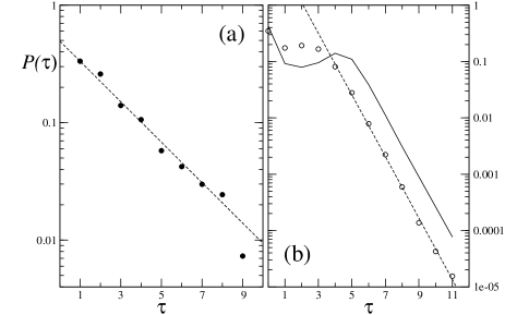
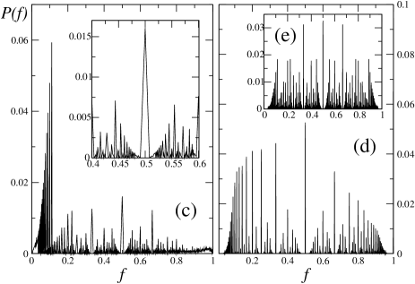
Figure 6: Distribution $P(\tau)$ of spreading times $\tau$ for (a) the Apollonian network of 8 generations, and (b) the real school network (circles) and the BA network with $m=9$ and $N=1000$ (solid line). The dashed lines indicate the best fit to the data for large $\tau$ values of Eq. (3), with parameters $(1-\gamma)/B=-0.45$ and $-1.26$ for the APL in (a) and the real school network in (b), respectively. Below, the distributions of $f$ are shown for (c) the BA network with the same parameter values (inset magnifies the range $f\in[0.4,0.6]$), for (d) the schools and for (e) an artificial distribution of all possible fractions $f$ among the same number of nodes and neighbors. The highly positive skewness in $P(f)$ of both BA and schools networks are in strong deviation with the artificial distribution, indicating a structure among the way neighbors connect with each other (see text).

To go further with the characterization of information spreading on networks, we next study the distributions, $P(\tau)$ and $P(f)$. In Fig. 6a we see that for the Apollonian network the distribution $P(\tau)$ of the spreading time decays exponentially. This behavior can be understood if we consider that $P(\tau)d\tau=P(k)dk$ and use Eq. (1) together with the degree distribution, $P(k)\propto k^{-\gamma}$, to obtain

$$P(\tau)\propto\exp{\tfrac{\tau(1-\gamma)}{B}},$$ (3)

for large $k$. The slope in Fig. 6a is precisely $(1-\gamma)/B=-0.17$ using $B=1.1$ from Fig. 4c and $\gamma=2.58$ from Ref. hans05 .

For the school network $P(\tau)$ follows an exponential decay for large $\tau$, as shown in Fig. 6b, and has a maximum for small $\tau$. For comparison, we also plot in Fig. 6b the distribution $P(\tau)$ for the BA network with $m=9$, which has a very similar shape but is shifted to the right, due to the larger minimal number of connections. In both cases, the distribution is well fitted by an exponential. The reason for the similiarities between empirical networks and BA networks at the particular value $m=9$ may be related to the way the questionnaire was made at the schools: each student should name their friends out of a maximal number of $10$ acquaintances. From the similarities we could now argue that in fact on average the students elected $9$ acquaintances each.

Figure 6c shows the distribution $P(f)$ for a scale-free BA network, while Fig. 6d shows the same distribution for the empirical networks. Before studying such distributions the following remarks should be taken into account. The spreading factor depends on the number $k$ of neighbors and consequently depends also on the network size, since the larger the network the larger the maximal number $k_{max}$ of neighbors a node may have. Furher, the spread factor varies always between the minimal value $0$ and the maximal value $1$ and for a given node with $k$ neighbors the possible values are $f=0,1/k,2/k,\dots,(k-1)/k,1$. Consequently, if for a specific network all the possible $f$-values appear with the same probability one should expect the distribution $P(f)$ to be symmetric around $f=1/2$ with discrete peaks at $n/k$ for $n=0,1,\dots,k$ and $k=1,\dots,k_{max}$. This artificial distribution is shown in Fig. 6e, obtained from all possible fractions constructed with all integers from $N=1$ to $1000$.

For BA networks, there is also a symmetry in the vicinity of $f=1/2$ (Fig. 6a). However, different from an uniform distribution, one finds a strong asymmetry between small and large values of $f$: the most pronounced peaks are observed for $f\lesssim 0.1$. This same behavior is observed for the empirical school networks, as shown in Fig. 6d, which is also strongly asymmetric when compared with the corresponding uniform distribution of all possible values of $f$ sketched in Fig. 6e. The positive skewnesses indicate a higher frequency of low $f$-values than of larger ones, which indicates in fact that the neighbors of nodes tend to form small separated sets of linked neighbors. Consequently, one is able to address how the connections between neighbors are groupped only by measuring the spreading factor for the central node. For the distribution $P(f)$ of the Apollonian network one trivially finds $P(f)=\delta(1-f)$ since the hierarchical structure of the network always yields $f=1$, as mentioned before.

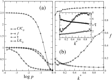
Figure 7: (a) Propagation of information in small-world networks: Spreading time $\tau$, clustering coefficient $C/C_{0}$ and spread factor $f$ as a function of the logarithm of the rewiring probability $p$ for the small-world lattice with $N=10^{4}$ sites. $C_{0}=1/2$ is the clustering coefficient of a regular lattice. In all cases we average over 100 configurations and $k_{0}=4$ (see text). (b) Dependence of the spread factor $f$ on $k^{*}=(k-k_{min})/(k_{max}-k_{min})$, for the random graph with $N=10^{3}$ sites and $p=0.02$ (circles), $0.04$ (squares) and $0.08$ (triangles). In the inset: the spreading time $\tau$ of the random networks for the same parameter values.

Social networks are usually small-world strogatznat , i.e., they are characterized by a high clustering coefficient and a low average shortest path length. Since we are interested in social systems we will next study the propagation of information on artificial small-world networks, constructed as follows strogatznat . One starts with a regular lattice where each node is attached to $k_{0}$ neighbors symmetrically displaced. Such regular network is characterized by a clustering coefficient $C_{0}$ and a shortest path length $L_{0}$. In this regular network, all links are short-range. Then, sweeping over all nodes one rewires with probability $p$ each link to a randomly chosen node. By doing this there will be on average $pk_{0}N/2$ long-range links.

For $p=0$ the network is a regular structure where no long-range links exist, yielding a large average path length and clustering coefficient. For $p=1$ all links are long-range producing a random graph structure where both average path length and clustering coefficient are small. Increasing $p$ from $0$ to $1$, one first observes the decrease of the shortest path length $L$, when compared to $L_{0}$, and only for larger values of $p$ the decrease of the clustering coefficient $C$, as shown in Fig. 7a. Therefore, in the middle range between the decrease of $L$ and the decrease of $C$ one obtains the small-world effect where $L/L_{0}$ is small and $C/C_{0}$ is large barabasirev . As shown in Fig. 7a this range is approximatelly $-2\lesssim\log{p}\lesssim-1$. In Fig. 7a one also sees that both the spread factor $f$ starts to decrease at approximately the same value of $p$ as the normalized clustering coefficient $C/C_{0}$.

Figure 7b illustrates the variation of the spread factor as a function of the degree in the particular case of a random network. Instead of the above procedure with $p=1$ fixed, random networks can also be constructed by starting with $N$ nodes and introducing with probability $p^{\prime}$ one link between each pair of nodes. Typically, in random networks there is a threshold $p^{\prime}_{c}$ beyond which different structure and dynamical features appear. This is also the case for gossip propagation. Figure 7b shows the behavior of $f$ in random networks for three illustrative values of $p^{\prime}=0.02,0.04$ and $0.08$, while the inset shows the corresponding spreading time. Since in random networks the average degree increases with $p^{\prime}$, we choose to compute $f$ and $\tau$ as functions of $k^{\ast}=(k-k_{min})/(k_{max}-k_{min})$ in order to facilitate comparison. For $p^{\prime}=0.02$ and lower values both the spread factor and spreading time remain approximately constant, with $f\sim 1/k$ and $\tau\sim 1$. Increasing the probability to $p^{\prime}=0.04$ increases the average degree per node and also the spread factor beyond its initial value $f=1/k$, and consequently the corresponding spreading time, $\tau>1$, increases with $k$. Increasing even further the probability to $p^{\prime}=0.08$ and beyond, more and more connections are introduced throughout the network, in particular among the neighbors of each node, which enables more nearest neighbors to know about the gossip. Consequently, on average one obtains $f_{\hbox{max}}=1$ independently of $k$. This maximal value for such values of $p^{\prime}$ means that the spreading attains all the neighbors of the victim. Therefore one should expect that the time to reach complete spreading should decrease with $k^{\ast}$, which is what one observes in the inset of Fig. 7b.

As a preliminary conclusion of this section one can state that, although different in their structure, empirical social networks behave similarly to scale-free networks when subject to propagation of information over the first neighborhood of a particular target-node.

III Beyond the first neighbors

In this Section we will study how $f$ and $\tau$ change when the information is able to propagate beyond first neighbors. For that, we consider two different regimes of information spreading. In the first regime, it spreads among the first and second neighbors of the victim, and in the second it spreads throughout the entire network. For the latter, there are two other quantities of interest that we introduce here. One is the total fraction $F_{N}$ of nodes who know and transmit the information, defined as

$$F_{N}=\frac{N_{g}}{N},$$ (4)

where $N_{g}$ is the maximal number of nodes in the entire network which already know the information and $N$ is the total number of nodes. Second, the maximal spreading time $\tau_{max}$ defined as the number of time-steps necessary to attain the fraction $F_{N}$.

Figure 8 shows the spreading dynamics in the American schools when it spreads among the two first neighborhoods of the victim. The behavior is significantly different from the one observed previously (compare with Fig. 5). From Fig. 8a one sees that the spreading time becomes independent on $k$ for large values deviating from the logarithmic dependence observed previously.

As for the spread factor $f$ shown in Fig. 8b, one still observes an optimal value minimizing the spreading of the gossip, but this value is now much lower than the one found for propagation only among common neighbors of the originator and the victim. Probably here, contrary to what happens in the previous case, the optimal value vanishes when the network size or the number of connections increase. This conjecture will be reinforced next by studying artificial scale-free networks.

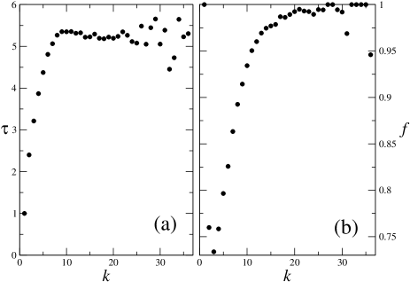
Figure 8: Information or gossip propagation through the first two neighborhoods in American schools: (a) Spreading time $\tau$ as a function of $k$ and (b) the spread factor $f$ as a function of $k$. As one sees the optimal number $k_{0}$ for which $f$ attains a minimum decreases significantly compared with the previous situation (see text).

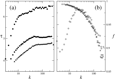
Figure 9: Propagation of information among first and second neighbors of a BA scale-free network. Here one sees (a) the spreading time $\tau$ as a function of the degree $k$ for $m=3$ (circles), $m=5$ (squares) and $m=7$ (triangles). (b) Spread factor $f$ for the same $m=3$ (circles), $m=5$ (squares) and $m=7$ (triangles). Here $N=10^{4}$, averages over $100$ realizations were considered and logarithmic binning in $k$ was used.

As illustrated in Fig. 9 the same behavior observed for the schools is also observed for BA networks. Here, the results for three different BA networks are shown for $m=3$ (circles), $m=5$ (squares) and $m=7$ (triangles). The spreading time $\tau$ attains also a constant value independent on $k$ for large $k$-values (Fig. 9a). Obviously this plateau decreases with the minimal number $m$ of connections and our simulations show that the dependence on $m$ is approximately logarithmic for small values of $k$. This decrease happens because increasing $m$ increases the number of links per node, enabling a faster propagation. Moreover the maximal value to which $\tau$ converges for large $k$ can be explained as follows: since now the information spreads over first and second neighbors, if the network has poor $k$-correlations, for sufficiently large $k$, all values of $k$ start to be present within the two first neighborhoods yielding an independence of $\tau$ on $k$. The distribution of the spreading time presents also an approximatelly exponential tail with a slope that increases with $m$.

As for the spread factor $f$, the optimal value $k_{0}$ is observed only for small $m$ ($m=3$) and rapidly vanishes when $m$ is increased. In fact, for large values of $m$ one finds large values of $f$ decreasing with $k$ as $f\propto 1/k$. This occurs independently of $m$. Due to the large values of $f$, the distribution $P(f)$ has again a very pronounced peak at $f=1$.

While for these BA networks the results are quite different when the two first neighbors are considered instead of only nearest neighbors, the Apollonian network displays an almost invariant behavior. for an Apollonian network almost the same behavior remains. The lack of sensibility to the increase of the neighborhood in Apollonian networks is a consequence of its hierarchical structure. Also for small-world and random networks similar results are obtained. So, as preliminary conclusions one sees that in hierarchical networks and in networks with small-world property it does not matter if the information can be transmitted beyond the victim’s acquaintances or not: in one way or another everyone rapidly knows our secrets!

After seeing what happens in small neighborhoods, the next question refers to the opposite limit, i.e., when all nodes are able to get the information from the originator. Of course in this case the fraction $f$ almost always achieves eventually its maximal value $f=1$, since the information eventually reaches everybody. This is a similar situation of what happens with the spread of rumours or epidemics. Though, there is still the case when some neighbor of the victim has no other friends and therefore the information cannot spread from or to it. The main question now is not only to know the minimal time $\tau$ needed for the information to reach the maximal number of nearest neighbors of the victim, but also to compare it with the maximal time $\tau_{max}$ needed for the information to achieve the maximal fraction $F_{N}$ (see Eq. (4)) of nodes which are reached.

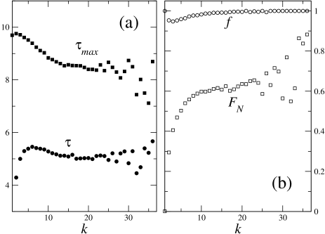
Figure 10: The spread of information through the entire school networks. (a) Spreading time $\tau$ and maximal spreading time $\tau_{max}$ as function of degree $k$. (b) Spread factor $f$ and total affected fraction $F_{N}$ as a function of $k$.

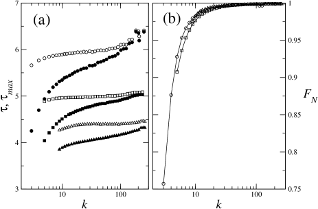
Figure 11: The propagation of information throughout an entire BA network. (a) the spreading time $\tau$ and maximal spreading time $\tau_{max}$ as a function of the degree $k$ for $m=3$ (circles), $m=5$ (squares) and $m=9$ (triangles). The total fraction $F_{N}$ of nodes that get the information is plotted in (b). In all cases, $f=1$ always (see text). Here $N=10^{3}$, averages over $100$ realizations were considered, and logarithmic binning in $k$ was used.

For the school networks, the behavior is illustrated in Fig. 10. From Fig. 10a one sees that the behavior of $\tau$ is almost the same as in Fig. 8a. The maximal time decreases with $k$ before attaining an approximatelly constant value. The large fluctuation for $k>25$ is due to poor statistics. The decrease of $\tau_{max}$ for small $k$ occurs, since for victims with less friends the successive neighborhoods through which the information spreads comprehend a smaller amount of neighbors than when starting with a larger number of friends.

As explained above the spread factor is approximatelly one independently of $n$, yielding a delta distribution $P(f)\sim\delta(1-f)$, while the maximal fraction $F_{N}$ increases fast for small $k$ and rapidly attains a more or less constant value around $F_{N}\sim 0.6$. Therefore, no optimal number of friends is observed.

Figure 11 shows what happens in the BA case. As one sees from Fig. 11a, both $\tau$ and $\tau_{max}$ decrease with $m$. Further, for both quantities, $\tau$ (black symbols) and $\tau_{max}$ (white symbols), a fast convergence to a logarithmic dependence on $k$ is observed when $k$ increases. Interestingly, while the slope as a function of $\log{k}$ differs between $\tau$ and $\tau_{max}$, in each case it is approximately independent of $m$, being apparently a feature of the scale-free topology.

In this situation one has always $f=1$. As for $F_{N}$, very large values are now observed ($F_{N}>0.7$) independently of $k$ and $F_{N}$ increases very fast attaining $F_{N}\sim 1$ for $k>10$ neighbors (see Fig. 11b). In other words, on BA networks, in order that all neighbors of a certain victim get the information, it must spread throughout the entire network.

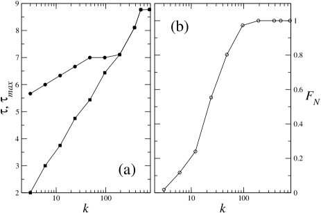
Figure 12: Propagation of information on an Apollonian network with $n=8$ generations: (a) Minimal time $\tau$ and maximal time $\tau_{max}$ and (b) the fraction $F_{N}$ between the total number of nodes which are reached by the information and the total number $N$ of nodes, both as functions of $k$. Here, $P(\tau)\propto P(\tau_{max})\propto P(k)\propto k^{-\gamma}$ (see text).

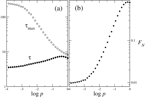
Figure 13: Information propagation in small-world networks when it spreads over the entire network. (a) Spreading time $\tau$ and maximal time $\tau_{max}$ and (b) total fraction $F_{N}$ as a function of the rewiring probability $p$. Here $N=10^{3}$ nodes and averages over $100$ realizations were considered.

Figure 12 illustrates the case of the Apollonian network. The value of $\tau_{max}\geq\tau$ increases more slowly with $k$, being both quantities equal for very large $k$ values. This similarity between both spreading times $\tau\sim\tau_{max}$ is in fact another evidence for the fact that in order to enable the information to reach all neighbors it must spread throughout the entire network. In fact, from Fig. 12c one also sees that in the range where $\tau_{max}>\tau$, $F_{N}<1$, being equal to one only in the range $\tau=\tau_{max}$.

Finally, we examine the case of small-world networks illustrated in Fig. 13. From Fig. 13a one sees that the spreading time $\tau$ increases almost linearly with the rewiring probability $p$ except at the end for large values of $p$ (random network). The maximal spreading time $\tau_{max}$ is very large for low rewiring probabilities, due to a large average path length, and decreases one order of magnitude in the range $-2<\log{p}<-1$ corresponding to small-world networks. In fact, $\tau_{max}$ follows the dependence of the average path length on $p$.

As for the total fraction $F_{N}$ illustrated in Fig. 13b one finds the opposite dependence on $p$ than the one found for $\tau_{max}$: for low (large) values of $p$ one finds low (large) values of $F_{N}$, and a pronounced increase is observed throughout the entire small-world regime. To explain this behavior one must use both the average path length and the clustering coefficient, $L/L_{0}$ and $C/C_{0}$ shown in Fig. 7a. For random networks ($p=1$) the total fraction attains $F_{N}=1$ very fast due to the very short average path length. For small values of $p$, although regular networks have an average path length that is larger than in random networks, the spreading time needed to attain $F_{N}=1$ is now proportional to $L$. In the small-world regime however, the average path length is small but the way the neighbors are connected isolates in some few cases nodes from the information spreading process. So, although small-world networks have large cluster coefficients as in regular networks, the long-range connections change significantly the local topology of a given node-neighborhood.

IV Introducing a transmission probability

In all the previous results each friend will surely spread the gossip further. Fortunately people are on average not as nasty as that. One should expect that only a certain fraction $q<1$ of our friends are not worth to be trusted. In this Section we address this more realistic situation.

Since we do not have any sociological information about the topological features of the ‘good’ friends we introduce $q$ as a probability that a node has to spread the gossip. For the particular case $q=1$ one reduces to the situations studied previously.

Two possible ways of propagation may then occur. One concerns a scenario where friendships connections are related to contacts between the nodes at a given instant. In this situation a certain individual tries only once, with probability $q$, to spread the information to its friends. Therefore, if the gossip is not ‘accepted’ once it will never be. Another scenario is of course when the spread is tried repeatedly at each time-step. We will start with this latter scenario and end with the more pleasant one where gossip is only able to spread from the nodes which heard it most recently.

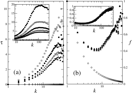
Figure 14: Information or gossip propagation among first neighbors with probability $q$ on a real friendship network of American students schools averaged over 84 schools. In (a) we show the spreading time $\tau$ and in (b) the spread factor $f$, both as function of degree $k$. The insets show the same data for the BA network with $m=9$ and $N=1000$. At each time-step each node which knows the gossip tries to spread it. In all plots one has $q=0$ ($\circ$), $q=0.2$ ($\bullet$), $q=0.4$ ($\square$), $q=0.6$ ($\blacksquare$), $q=0.8$ ($\triangle$) and $q=1$ ($\blacktriangle$).

Introducing the new parameter $q$ in the model we go back to the first information spreading model studied in Section II where the gossip only spreads to friends of the victim. At each time-step the neighbors which already know the gossip repeatedly try to spread it to other friends of the victim. Therefore, one expects to attain the same value of $f$ that one measured for $q=1$, but this time only after a larger spreading time, namely $\tau^{\prime}=\tau/q$. Figure 14 shows the result of such information propagation regime for the school networks. and for several values of $q$. The corresponding curves of $f$ are plotted in Fig. 14b.

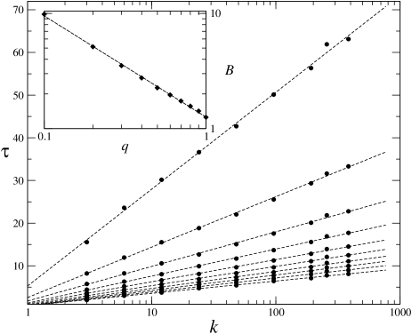
Figure 15: Gossip propagation in an Apollonian network with $n=8$ generations, for $10$ values of probability $q=0,0.1,0.2,\dots,0.9$ and $1$. The slope $B$ of the dashed lines which fit the data decreases with $q$ as shown in the inset where the line yields $B=\exp{(0.23-0.88\log{q})}\sim 1/q$ (see text).

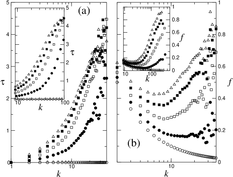
Figure 16: Propagation of gossip among first neighbors on a real friendship network of American students schools , when persons to which a gossip did not spread at the first attempt will never get it. In (a) we show the spreading time $\tau$ and in (b) the spread factor $f$, both as a function of degree $k$. The insets show the same data for the BA network with $m=9$ and $N=1000$. After knowing the gossip each node tries to spread it only once (see text). In all plots one has $q=0$ ($\circ$), $q=0.25$ ($\bullet$), $q=0.5$ ($\square$), $q=0.75$ ($\blacksquare$) and $q=1$ ($\triangle$).

Of course for $q=0$ the spreading time is always $\tau=0$ and the spread factor equals $f=1/k$ since only the node starting the gossip will know it. As expected, for all other values the spread factor coincides with the one for $q=1$, while the spreading time preserves its logarithmic dependence on $k$ for large degrees, and the exponent increases with $1/q$,as explained below.

In the insets of both plots in Fig. 14 we show for comparison the spreading time $\tau$ and spread factor $f$ for a BA network with $N=1000$ and $m=9$. A strong deviation from the logarithmic dependence of the spreading time is observed, due to the high number of initial outgoing connections ($m=9$).

The logarithmic dependence of the spreading time can be more easily seen when studying the Apollonian network as shown in Fig. 15. Here we plot the spreading time for $10$ different values of $q$ and fit all of them with a logarithmic function as the one in Eq. (1). The corresponding slope $B$ as a function of $q$ is plotted in the inset of Fig. 15 and follows closely a hyperbolic behavior, $B\sim 1/q$. Thus, Eq. (1) can be written more generally as

$$\tau\propto\tfrac{1}{q}\log{k}.$$ (5)

Finally, we can also assume that the person to which a gossip did not spread at the first attempt, will never get it. In this way, the gossip is a quantity which percolates through the system.

In Fig. 16 we see the behavior of $\tau$ and $f$ for different values of $q$ for the school networks and in the inset for the BA network. When the spreading probability $q$ decreases, the minimum in $f$ first shifts to larger $k$ and finally disappears. The asymptotic logarithmic law of $\tau$ for large $k$ remains for all probabilities $q$. As in previous cases, the BA network has a similar behavior as the school friendships. The Apollonian network, however, behaves quite differently: $\tau$ first increases with $q$ and then eventually falls off to zero so that there exists a special value $q_{max}\approx 0.75$ for which the spreading time $\tau$ is maximized.

V Discussion and conclusions

In this paper, we studied a general model of information spreading suited for different kinds of social information. In the usual case of rumour or opinion propagation the information spreads throughout the network, and all nodes are equally capable of transmiting the information to their neighbors. Two measures were proposed to characterize the spreading of such model, namely, the spreading factor measuring the accessible neighborhood around each node which can be reached by the information spreading, and the spreading time which computes the minimum time to reach such neighborhood.

Further, we have shown that by computing these quantities for each node the resulting distributions give additional insight to the underlying network structure on which the spreading takes place. More precisely, the magnitude of the skewness of the distribution of the spreading factor gives a measure of how difficult it is to access one neighbor, starting from another one. For positive values of the skewness, most of the pairs of neighbors are connected by some path of connections, while for negative values of the skewness, neighbors are more likely groupped in separated connected pairs.

In the particular case that the information is about a certain target-node and thus is of interest to a restricted neighborhood around it, one yields a minimal model to study gossip spreading. Applying such a scheme to artifical and empirical networks, we found that, although different in their statistical properties, information on empirical social networks seems to spread similarly to what is observed in scale-free networks. In both cases, the spreading time shows a logarithmic dependence on the degree, indicating small-world effect within the nearest neighborhood of the nodes. Further, from the computation of the spreading factor we observed that there is a non-trivial optimal number of friends which minimizes the danger of being gossipped that depends on the size of the network and on total number of acquaintances in it. We also showed that this optimal value is characteristic of either scale-free networks or real social networks, but is not observed in small-world networks, rising the question of what network properties may give rise to the emergence of such an optimal value.

However, when the information spreads beyond the nearest neighbors, in a similar way as for propagation of rumours and epidemics, this optimal value disappears with the spreading factor rapidly converging to $f=1$. Also the logarithmic dependence of the spreading time no longer holds in this case.

Since one person does not in general spread information to all its neighbors, neither at the same time nor with complete certainty, we also studied regimes of information propagation where the spreading from one node to another occurs with some probability $q$.

Due to their particular features and assumptions, our concepts and measures to address the propagation of information in networks could be suited to other situations. For instance, in the case of the Internet, some trojan horses need to connect to a specific host to download some data in order to become effective. For them the spread factor should be a good measure to assess the vulnerability to the spreading of this virus attack. In this situation probably an experimental test of the emergence of the optimal degree found in the cases stated here could be easier to be implemented.

References

- (1) J. S. Andrade Jr., H.J. Herrmann, R.F.S. Andrade, L.R. da Silva, Phys. Rev. Lett. 94, 018702 (2005).
- (2) A.D. Sánchez, J.M. López and M.A. Rodríguez, Phys. Rev. Lett. 88, 048701 (2002).
- (3) P.L. Krapivsky and S. Redner, Phys. Rev. Lett. 90, 238701 (2003).
- (4) M. Mobilia and S. Redner, Phys. Rev. E 68, 046106 (2003).
- (5) S. Boccaletti, V. Latora, Y. Moreno, M. Chavez and D.-U. Hwang, Physics Reports 424, 175-308 (2006).
- (6) C.G. Shao, Z.Z. Liu, J.F. Wang and J. Luo, Phys. Rev. E 68, 016120 (2003).
- (7) P.G. Lind, M.C. González and H.J. Herrmann Phys. Rev. E 72, 056127 (2005).
- (8) P.S. Dodds and D.J. Watts, Phys. Rev. Lett. 92, 218701 (2004).
- (9) C. Castellano, M. Marsili, A. Vespignani, Phys. Rev. Lett. 85, 3536-3539 (2000).
- (10) A. Pluchino, V. Latora and A. Rapisarda, Int. J. Mod. Phys. C 16(4), 515-531 (2005).
- (11) S. Galam, Phys. Rev. E 71, 046123 (2005).
- (12) M. He, H. Xu and Q. Sun, Int. J. Mod. Phys. C 15(7), 947-953 (2004).
- (13) V.M. Eguíluz and M.G. Zimmermann, Phys. Rev. Lett. 85, 5659-5662 (2000).
- (14) P.G. Lind, J.S. Andrade Jr., L.R. da Silva, H.J. Herrmann, Eur. Phys. Lett. accepted (2007); cond-mat/0603824.
- (15) Add Health program designed by J.R. Udry, P.S. Bearman and K.M. Harris funded by National Institute of Child and Human Development (PO1-HD31921).
- (16) H.J. Herrmann, D.C. Hong and H.E. Stanley, J.Phys.A 17, L261 (1984).
- (17) D.J. Watts and S.H. Strogatz, Nature 393, 440-442 (1998).
- (18) L.A.N. Amaral, A. Scala, M. Barthélemy and H.E. Stanley, Proc. Nat. Acad. Sci. USA 97, 11149 (2000).
- (19) M.C. González, P.G. Lind and H.J. Herrmann Phys. Rev. Lett. 96, 088702 (2006); cond-mat/0602091.
- (20) M.M. Telo da Gama and A. Nunes, Eur. Phys. J. B, 50, 205 (2006).
- (21) A.-L. Barabási and R. Albert, Science 286, 509-512 (1999).
- (22) S.N. Dorogovtsev, A.V. Goltsev and J.F.F. Mendes Phys. Rev. E 65, 066122 (2002).
- (23) P.G. Lind, J.A.C. Gallas and H.J. Herrmann, Phys. Rev. E 70, 056207 (2004).
- (24) P.S. Bearman, J. Moody and K. Stovel, Am.J. of Soc. 110, 44 (2004).
- (25) M.C. González, P.G. Lind and H.J. Herrmann Physica D 224 137 (2006).
- (26) M. Cantazaro, M. Boguña and R. Pastor-Satorras, Phys. Rev. E 71 027103 (2005).
- (27) M. Cantazaro, M. Boguña and R. Pastor-Satorras, Phys. Rev. E 71, 056104 (2005).
- (28) D.J. Watts and S.H. Strogatz, Nature 393, 440-442 (1998).
- (29) R. Albert and A.-L. Barabási, Rev. Mod. Phys. 74, 47-97 (2002).