Study of sediment transport in the saltation regime

F. Osanloo¹, M. R. Kolahchi¹, S. McNamara ², H. J. Herrmann³

1. Institute for Advanced Studies in Basic Sciences, P. O. Box 45195-1159, Zanjan, Iran

2. Institute for Computer Physics, Stuttgart University, 70569 Stuttgart, Germany

3. Computational Physics, IfB, ETH Zürich, Hönggerberg, 8093 Zürich, Switzerland

We present a study of sediment transport in the creeping and saltation regime. In our model, a bed of particles is simulated with the conventional event-driven method. The particles are considered as hard disks in a 2d domain, with periodic boundary conditions in horizontal direction. The flow of the fluid over this bed of particles is modeled by imposing a force on each particle that depends on the velocity of the fluid and its height above the bed. We considered two velocity profiles for the fluid, parabolic and logarithmic. The first one models laminar flow and the second corresponds to turbulent flow. For each case we investigated the behavior of the saturated flux. We found that for the logarithmic profile, the saturated flux shows a quadratic increase with the strength of the flow, and for parabolic profile, a cubic increase. The velocity distribution functions are used to interpret the results.

1 Introduction

The study of transport of granular material by a fluid is important for industrial processes as well as understanding of natural phenomena. Modeling of the sediment transport in rivers, as well as modeling of sand drift in the formation of dunes, benefits from this study. Saltation, surface creep, and suspension are three modes which occur during transportation of granular material by a fluid[1]. When the shear velocity of the fluid flowing over a bed of grains exceeds the friction threshold velocity for sand transport, the grains are driven by the fluid. At first they begin to move while still in continual contact with each other, yet it could happen that every now and then due to collisions, some particles jump by a distance of order of their diameter. This regime is called surface creep or reptation. As the fluid shear velocity increases, the particles can follow paths that take them to a height much larger than the grain diameter; this regime is called saltation. The grains in saltation have been named saltons, and the grains in creeping motion have been named reptons [2]. Suspension occurs at very high shear velocities, when a considerable fraction of the particles are transported upwards by turbulent eddies. In this regime, the grains move in the fluid for long periods of time, hardly colliding with the bed or each other. Except for dust storms in which suspension is dominant, creeping and saltation of sands usually play the key role in dune formation [3]. In many of the experimental studies of sediment transport, grains are transported by air[3],[4], but few experiments in water also exist[5],[6]. To gain insight into the problem of sediment transport, it is important to understand the relation between the flux of the grains transported by the fluid and the velocity profile of the fluid that moves over the grains. In most instances of sediment transport, the flux eventually saturates at a certain strength or amplitude, $u_{*}$, of the velocity profile, $v(y)={u_{*}}f(y)$. Here, $f$ is a function of height, $y$. However, there are situations, as at the foot of a sand dune, where the sand flux may never reach saturation. In such cases, where there is no saturation the variation of flux can be studied [7]. Bagnold [1] was first to introduce a simple flux law, a cubic relation, expressing the behavior of sand flux with the shear velocity. Other forms for the flux law have also been proposed by different authors for different physical conditions[8],[9]. In this work, we study two profiles for the fluid flow, and concentrate on the saltation regime of the grain motion. We emphasize that for the purposes of this study, saltation has a different meaning than its standard usage. For instance, in a wind tunnel, a grain is in saltation if its trajectory is at least about 300 grain diameters high and at least 1000 grain diameters across. These are much larger than the size of the system considered here. Yet, we use this term to distinguish the motion from the situation where the grains constantly touch each other as they slowly move. Saltation is then used to mean a motion where the grains jump and follow a trajectory, albeit smaller than mentioned above. The structure of the paper is as follows. In Section II we introduce the model. Then in Section III, we study the behavior of the flux as a function of the velocity profile, as well as the velocity distribution functions for the grains. Section IV is devoted to our discussions which mainly rest upon the comparison of velocity distributions. Finally, we present our conclusions as Section V.

2 Simulation Model

We use the inelastic hard sphere model[10]. Grains are contained in a two dimensional rectangular domain with periodic boundary conditions in the horizontal directions. The fluid flows over the bed of grains, so grains can be entrained by the fluid. The fluid is modeled by its velocity profile. The grains, modeled as disks, move under the influence of both gravity and a drag force that is exerted on them by the fluid. To avoid crystallizations, $20\%$ of the particles have a diameter equal to $0.6l_{0}$ and the rest have a diameter equal to $0.5l_{0}$ where $l_{0}$ is the unit of length used throughout this paper. A gravitational acceleration of $12l_{0}/{t_{0}^{2}}$ is applied to all the particles, where $t_{0}$ is the unit of time [11]. All the particles have the same mass, and the effect of particles on the fluid is neglected.

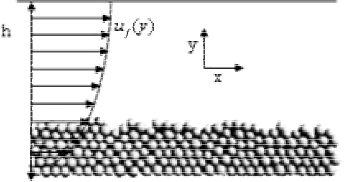
Figure 1: The schematic representation of the system showing the particles in their initial state, and the velocity field at different positions in the y-direction.

In all cases studied, the system starts out having six layers of particles resting fairly compactly on each other. The fluid stands at a height that is equivalent to thirty two layers, 16$l_{0}$. This height is the maximum attainable by the grains; because in our modellization we implement a reflecting boundary at the top so that the particles that touch it just reverse their vertical velocity component Fig.(1).

2.1 Particle Motion

We use event-driven MD [12] to calculate the motion of the particles. As the particles are hard spheres, collisions take infinitesimal time and involve only two particles. Conservation of momentum leads to

$$\vec{u}_{1,2} = \vec{v}_{1,2}\mp\frac{1+r}{2}\left(\hat{K}\cdot(\vec{v}_{1}-\vec{v}_{2})\right)\hat{K}$$ (1)

$$\mp \frac{1+\beta}{2}\left(\hat{t}\cdot(\vec{v}_{1}-\vec{v}_{2})\right)\hat{t},$$

where $\vec{u}$ indicates the velocities after the collision, and $\vec{v}$ denotes the velocities before the collision. The geometry of the collision is described by $\hat{K}$, a unit vector pointing along the line connecting the centers of particle $1$ to particle $2$, and $\hat{t}$ is the unit vector in tangential direction. The energy dissipation is measured by $r$, the normal restitution coefficient, and $\beta$, the tangential restitution coefficient. If $r=1$ and $\beta=\pm 1$, collisions conserve energy and are said to be elastic. For $0<r<1$ or $-1<\beta<1$ energy is dissipated and the collisions are inelastic. We assume that the particles neither rotate nor roll. This is somewhat in accord with the fact that the sand grains are not round which makes the rolling difficult. In our simulations, $r=0.4$ and $\beta=-1$. In using the event-driven method there are two problems in setting up the bed of grains: inelastic collapse, and creating a rough surface on the bottom. All particles after some collisions lose their energy and accumulate on the bottom and make a dense network of grains. So the number of collisions per unit time will diverge at finite time; that is, inelastic collapse [13] occurs. Because of the finite precision of the computer, multiparticle collisions can occur. For handling the inelastic collapse we use the Tc model with $t_{c}=10^{-6}t_{0}$ [13]. In order to create a rough surface, $r$ and $\beta$ are adjusted for collisions between the grains and the surface. We suppose that when a particle of the first layer bounces against the bottom plate both the tangential and normal components of its velocity are reversed, i.e, $r=1$ and $\beta=1$ in Eq.(1). In this way, the first layer is nearly fixed and acts as a rough surface over which other particles can move. The roughness is of the order of the particle diameter.

2.2 The Effect of Fluid on the Grains

The drag force is proportional to the difference between the particle velocity $\vec{u}_{p}$ and the fluid velocity $\vec{u}_{f}$.

$$\vec{F}=\gamma(\vec{u}_{f}-\vec{u}_{p}),$$ (2)

where $\gamma$ is a parameter that depends on the characteristics of both the fluid and the grains. In laminar flow with small Reynolds number, $\gamma=3\pi\eta d_{p}$, in which $\eta$ is the viscosity of the fluid and $d_{p}$ is the diameter of the particle. We suppose that $\gamma=1$ for laminar flow. However in turbulent flow, the fluid drag varies as the square of the grain speed and $\gamma$ can be written as:

$$\gamma=\frac{3C_{D}\rho_{f}}{4\rho_{p}d_{p}}\mid{\vec{u}_{f}-\vec{u}_{p}}\mid,$$ (3)

which corresponds to the Newtonian drag force where, $C_{D}$ is taken from empirical relations, $\rho_{f}$ and $\rho_{p}$ are the density of the fluid and particle respectively. In general, the drag force acts on upper layers of the bed of particles and drops to zero for lower layers. The details depend on the velocity profile considered. Here, we study the dynamics of the grains for two velocity profiles: logarithmic and parabolic. For the parabolic profile, which models laminar flow in open channels as function of height, we have:

$$u_{f}={u_{*}}(y_{0}(y_{0}/2-h)-y(y/2-h)),$$ (4)

where $h$ is the height of fluid in channel. This equation is written so that it satisfies the two boundary conditions, $\partial u_{f}/\partial y=0$ at $y=h$, and $u_{f}=0$ at $y=y_{0}$. Here, $y$ is the height, and $y_{0}$ is the height below which the effect of the fluid on the grains is negligible. In turbulent flow, the velocity profile of the fluid near the boundary is observed to be logarithmic[14], and described by

$$u_{f}={\frac{u_{*}}{k}}log(y/y_{0}),$$ (5)

where $k$ is the von Karman constant. Although this relationship has been derived only for the region in which the shear stress is approximately constant, experiments show that the agreement persists through almost all of the boundary layer. In our simulations, $y_{0}$ is about the diameter of grains, $y_{0}=0.5l_{0}$. We consider no vertical component to the fluid velocity.

3 Granular Flux and Velocity Probability Distribution Function

First we investigate the behavior of the granular flux with respect to time. Granular flux is the number of grains that cross the unit surface (unit line in 2d ) per time unit. So the flux integrated over a cross section of the periodic domain (over height in 2d) is:

$$q=\frac{1}{L}\sum_{i=1}^{N}u_{i},$$ (6)

where $L$ is the length of the box and $N$ is the total number of particles, and $u_{i}$ denotes the horizontal component of the velocity of the $i$th particle. After some time the flux fluctuates around a constant, steady value, and sediment transport reaches steady state. This steady state is the saturated flux, and it depends on the shear velocity, denoted by $u_{*}$. For calculating the saturated flux value, we average over the flux only after the steady state has been reached. We expect to have a threshold velocity $u_{t}$, below which sediment transport cannot happen.

3.1 Logarithmic Profile

Figure 2: Flux as a function of time for different values of $u_{*}$ for a logarithmic profile.

In the aeolian case the logarithmic velocity profile is more realistic than the parabolic profile. When the wind blows over a rough surface, its velocity within the boundary layer increases logarithmically with height, Eq.(5). The logarithmic profile has also been observed experimentally, for water moving over a rough surface in a channel [5, 6]. Fig.(2) shows the variation of flux with time for different values of shear velocity, $u_{*}$. This figure shows that transport process reaches steady state and the particle flux saturates after some transient time. The simulations could be made into movies of the grain motion. This was a particularly useful way of interpreting the results. In this way we estimate the grain motion to start at a threshold velocity of about $u_{*}=1$. With increasing $u_{*}$ from $u_{t}=1$, the top layer particles begin to roll in their own layer or jump to a height about their diameter. This situation continues until $u_{*}\simeq 15$. This means that for $u_{*}<15$ most of the particles except those in the bottom layer are in the creeping regime. After $u_{*}>15$ the shear stress is enough to make some of the particles in the upper layers enter the saltation regime. With increasing $u_{*}$, the number of saltating particles increases, resulting in an increase in the number of collisions between saltons. We estimate $u_{*}\simeq 15$ as marking the onset of saltation in this system. When $u_{*}>30$ enough particles have so high an energy that they move with the fluid stream above the other particles and have few collisions with each other or the rest of the grains. In this case the length of their trajectory becomes comparable to the system size, hence we only considered $u_{*}<30$. We wish to emphasize again that we are using the term saltation in a restricted sense in this study. The main objective of this study is to relate the saturated flux and the shear velocity in the regime of saltation. Our results for the behavior of the mean flux of particles with $u_{*}$ is shown in Fig.(3).

Figure 3: Mean flux vs. $u_{*}$ for a logarithmic profile, and the fit to it, Eq. (10) and Bagnold’s expression. Fit the Eq. (10) gives $a=0.2$, $b=43.9$, and $u_{t}=1.09$. According to the simulations we estimate $u_{t}=1$.

Theoretically, perhaps the most important description for saturated flux is due to Bagnold [1]. He found that the saturated flux at large shear velocities is given by:

$$q=\frac{\rho_{air}}{g}u_{*}^{3}.$$ (7)

Bagnold considered a mean trajectory for each grain, and supposed that the ejection velocity of grains from the bed scales with the shear velocity $u_{*}$. This hypothesis is valid if the shear velocity is large enough. For small shear velocities, Ungar & Haff [17] supposed that height and length of the trajectory of grains is of the same order as the grain size, and predicted that:

$$q\propto\rho_{air}(u_{*}^{2}-u_{t}^{2})\sqrt{\frac{d}{g}},$$ (8)

where $d$ is the grain diameter. Almeida et al.[15] also found numerically a quadratic description for the flux near the threshold shear velocity,

$$q\propto(u_{*}-u_{t})^{2}$$ (9)

They simulated the saltation inside a two-dimensional channel with a mobile top wall. Their model solves the turbulent wind field including feedback of the dragged particles. Our results show a slightly different quadratic dependence:

$$q=a(u_{*}-u_{t})(u_{*}+b)$$ (10)

where $a=0.2$, $b=43.9$, and $u_{t}=1.09$ are obtained from fitting the Eq.(10) to our data. This value for the threshold velocity is in good agreement with what was estimated from the simulations; that is $u_{t}=1$. Fig.(3) shows the fit, Eq. (10), to the data. This indicates that both in the creeping regime and the saltating regime, the same quadratic function describes the behavior of flux reasonably well. Eq. (10) predicts a stronger dependence on shear velocity, compared to Eq. (9). One reason may be our neglect of the back action of the grains on the fluid. This effect is more prominent at small heights above the bed where the particle velocity differs much from the fluid velocity [15]. Another way to estimate the onset of saltation is to investigate the behavior of the grain velocity probability distribution function. The distribution function allows decomposition of the flux into a part due to saltation and another part due to creep. This interpretation is based on the fact that the reptons are slower than the saltons. Fig.(4) shows the behavior of the grain velocity distribution for different values of $u_{*}$.

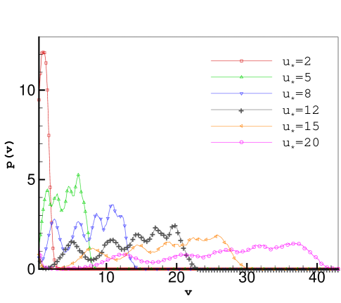
Figure 4: The behavior of grain velocity probability function for different values of $u_{*}$ for the logarithmic profile.

For small values of $u_{*}$ there is a large peak at small velocities that shows that all of the particles are in creeping motion. With increasing $u_{*}$, the velocity of the moving particles increases and some of the particles enter the saltation regime. The uniform distribution function at higher velocities represents the saltating particles. At $u_{*}=15$ the particles can go to the saltation regime; the velocity distribution develops a minimum at $v\sim 1$. At $u_{*}\sim 20$ all of particles have saltating motion.

3.2 Parabolic Profile

At low Reynolds numbers when a fluid flows in an open channel , its velocity varies with height parabolically. Now, we consider a velocity profile as in Eq.(4), that is zero at the bottom and increases parabolically with height.

Figure 5: Flux as a function of time a for parabolic profile.

Fig.(5) shows the behavior of flux as a function of time. Similar to the logarithmic profile, the flux reaches steady state, only now the transient time is longer. In the parabolic profile, the shear stress above the bed is greater than the logarithmic profile and increases rapidly with $u_{*}$, so compared to the logarithmic case, the range of $u_{*}$ that defines the creep motion is much narrower. The motion starts out at about $u_{t}=0.08$ [16]; this is an estimate obtained from our simulations, and in Eq.(12) below is used as an input data. When $u_{*}=1$ the system is out of the creeping regime, and starts saltating. The surface $y=h$ is as before a reflecting surface, so any particle that reaches it bounces back into the fluid. This starts at about $u_{*}=1.2$. Beyond $u_{*}=2.5$ this boundary produces a kind of population inversion and the collision of particles with each other effectively reduces the rate of increase of flux Fig. (6).

Figure 6: Mean flux as a function of $u_{*}$ for a parabolic profile. The solid line is our data, and the dashed line is fitting a cubic function to data. Beyond $u_{*}\sim 2.5$ the effect of the ‘top boundary‘ is revealed. $u_{t}=0.08$ is estimated from the simulations.

Figure 7: Mean flux as a function of $u_{*}$ near the threshold value $u_{t}=0.08$ for a parabolic profile. For $u_{*}<1$ we fitted the data with two Eqs.(11) , (12). The solid line is the fit using Eq. (12) yielding $a=182$, $b=-0.07$, and $c=0.5$. The dashed line is the fit using Eq. (11) that gives $a^{\prime}=258$, and $u_{t}=0.036$.

In fig.(7) we show the behavior of the mean flux with $u_{*}$ (near $u_{t}$). For $u_{*}<1$ we fitted the data with two equations below:

$$q = a^{\prime}(u_{*}-u_{t})^{2}$$ (11)

$$q = a(u_{*}-0.08)(u_{*}^{2}+bu_{*}+c)$$ (12)

The values of $a^{\prime}=258$, $a=182$, $b=-0.07$, $c=0.5$, and $u_{t}=0.036$ are obtained from fitting. The cubic equation is clearly a better fit to the data than the quadratic one.

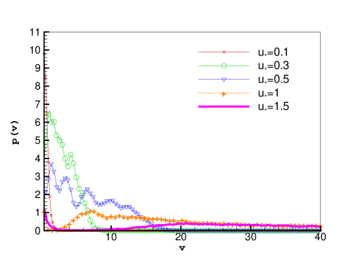
Figure 8: The behavior of the grain velocity probability function for different values of $u_{*}$ for a parabolic profile.

Fig.(8) shows the behavior of the grain velocity distribution for the parabolic profile. In this case, the saltation regime starts at $u_{*}=1$, below which all particles are in creeping motion. Beyond $u_{*}=1.5$, all particles are in the saltation regime.

4 Discussion

The dynamics of the granular systems under shear is usually studied for slow or quasi static flow [18]. Slow shearing can lead to the emergence of internal ordering of the granular systems. In terms of our study, this means the creeping regime. In fact we have also observed size segregation for the case of the logarithmic profile when the shear is small enough. Two granular materials differing by their size, exhibit a propensity for segregation. Whenever this mixture undergoes a vibration or a shearing action, the components tend to separate partially or completely [19]. Here we considered a system with two different sizes, differing in ratios by a factor 2, initially distributed randomly. When this system is affected by the drag force of the fluid, the two components of the system separate so that large particles will come to the top. In the creeping regime due to the higher collision rate, this separation occurs very soon. Overall, the present study considers the intermediate region, between the quasi static flow and the rapid flow. Due to finite size effects, we use the term ‘saltation’, to mean a motion that takes a particle on a trajectory, however small, raises it from the bed of grains. We interpret the results using the grain velocity distribution function, $P(v)$. With increasing shear we expect to have more and more particles in motion. The distribution function, $P(v)$, develops a peak at low velocities, $v\sim 2$, that gradually disappears as $u_{*}$ increases. In case of the logarithmic profile, this peak does not broaden. With the diminishing of this low energy peak, a plateau is developed in the velocity distribution. This plateau gradually covers a larger range of velocities. This plateau corresponds to saltons. The density of particles in the saltation regime, for the logarithmic profile, is a monotonically decreasing function of height. We attribute this to the comparatively smaller energy input rate; the latter going as $q_{f}u_{f}^{2}$, where $q_{f}$ is the fluid flux. For the parabolic profile, the situation is markedly different. We observe that as the shear velocity increases, the distribution develops a tail, covering the larger velocities. The rate of energy input is much higher in the case of the parabolic profile. In the saltation regime $(u_{*}\geq 0.8)$, it is possible to distinguish a group of particles that moves at a higher velocity and height, nearly separating from the rest of the particles. In this sense, the density of particles in the saltation regime, is qualitatively different from that of the logarithmic velocity profile. This explains the sudden velocity spread at $u_{*}\geq 0.8$.

5 Conclusion

In this study, we have presented a simple model for sediment transport in creeping and saltating motion that produces steady sediment transport. We investigated the steady state fluxes for the parabolic and logarithmic fluid velocity profiles. For the logarithmic profile we compared our results with some previous studies. Increasing the shear velocity $u_{*}$ from threshold value $u_{t}$, sediment transport sets in, first creeping and for larger $u_{*}$, saltating. In our system, the saltating particles can rise up to several times their diameter, and similar to the Ungar and Haff we find that the steady state flux increases quadratically with shear velocity. For the parabolic distribution the flux rises cubically with increasing the shear velocity. The velocity probability distribution function is a good measure to estimate the onset of the saltation. It would be interesting to study a system large enough so that the grain velocity distribution function can be measured as a function of height. Acknowledgment Part of this work was carried out while F. Osanloo stayed at the University of Stuttgart. She wishes to thank the University of Stuttgart for their hospitality and the grant that made her stay possible.

References

- [1] R.A. Bagnold The Physics of Blown Sand and Desert Dunes, Chapman and Hall, 1941.
- [2] B. Andreotti, P. Claudin, S. Douady, Eur. Phys. J. B 28, 321 (2002).
- [3] You-He Zhou, Xiang Guo, and Xiao Jing Zheng Phys. Rev. E 66, 021305 (2002).
- [4] K. Nishimura, and J. C. R. Hunt, J. Fluid Mech. 417, 77 (2000)
- [5] C. Ancey, F.Bigillon, P.Frey, and R. Ducret Phys. Rev. E 66, 036306 (2002).
- [6] C. Ancey, F.Bigillon, P.Frey, and R. Ducret Phys. Rev. E 67, 011303 (2003).
- [7] G. Sauermann, K. Kroy, and H. J. Herrmann , Phys. Rev. E 64, 031305 (2001)
- [8] K. Lettau and H. Lettau, Exploring the World’s Driest Climate, edited by H. Lettau and K. Lettau (Center for Climate Research, University of Wisconsin, Madison, 1978).
- [9] M. Sorensen, Acta Mech., Suppl. 1, 67 (1991).
- [10] S. McNamara and W. R. Young, Phys. Rev. E 53, 5089 (1996).
- [11] Throughout this paper the unit of length is , and the gravitational acceleration of is applied to all the particles. This is the acceleration experienced by a particle with density of in water. The corresponding unit of time is .
- [12] B.D. Lubachevsky, J. Comput. Phys. 94, 255 (1991).
- [13] S. Luding and S. McNamara, Granular Matter 1, 113. (1998).
- [14] A. Vardy Fluid Principles, McGraw- Hill, 1990.
- [15] M. P. Almeida, J. S. Andrade, Jr. H. J. Herrmann Phys. Rev. Lett. 96, 018001 (2006).
- [16] Although the threshold velocities for the two profiles are drastically different, the resulting drag forces (for the top layer), using Eqs. (2) through (5), come out nearly the same for both profiles, as expected, at the onset of motion.
- [17] B. Andreotti, J. Fluid Mech. 510, 47 (2004).
- [18] J. P. Gollub, J. C. Tsai, in Powders Grains 2005 (Balkema 2005), p. 743.
- [19] J. B. Knight, H.M. Jaeger, S. R. Nagel Phys. Rev. Lett. 70, 3728 (1993).