Configurations of saddle connections of quadratic differentials on $\mathbb{CP}^{1}$ and on hyperelliptic Riemann surfaces

Abstract.

Configurations of rigid collections of saddle connections are connected component invariants for strata of the moduli space of quadratic differentials. They have been classified for strata of Abelian differentials by Eskin, Masur and Zorich. Similar work for strata of quadratic differentials has been done in Masur and Zorich, although in that case the connected components were not distinguished.

We classify the configurations for quadratic differentials on $\mathbb{CP}^{1}$ and on hyperelliptic connected components of the moduli space of quadratic differentials. We show that, in genera greater than five, any configuration that appears in the hyperelliptic connected component of a stratum also appears in the non-hyperelliptic one.

1. Introduction

We study flat surfaces having conical singularities of angle integer multiple of $\pi$ and $\mathbb{Z}/2\mathbb{Z}$ linear holonomy. The moduli space of such surfaces is isomorphic to the moduli space of quadratic differentials on Riemann surfaces and is naturally stratified. Flat surfaces corresponding to squares of Abelian differentials are often called translation surfaces. Flat surfaces appear in the study of billiards in rational polygons since these can be ”unfolded” to give a translation surface (see [KaZe]).

A sequence of quadratic differentials or Abelian differentials leaves any compact set of a stratum when the length of a saddle connection tends to zero. This might force some other saddle connections to shrink. In the case of an Abelian differential this correspond to homologous saddle connections. In the general case of quadratic differentials, the corresponding collections of saddle connections on a flat surface are said to be ĥomologous (pronounced “hat-homologous”). According to Masur and Smillie [MS] (see also [EMZ, MZ]), a “typical degeneration” corresponds to the case when all the “short” saddle connections are pairwise ĥomologous). Therefore the study of configurations of ĥomologous saddle connections (or homologous saddle connection in the case of Abelian differential) is related to the study of the compactification of a given stratum. A configuration of ĥomologous saddle connections on a generic surface is also a natural invariant of a connected component of the ambient stratum.

In a recent article, Eskin, Masur and Zorich [EMZ] study collections of homologous saddle connections for Abelian differentials. They describe configurations for each connected component of the strata of Abelian differentials. Collections of ĥomologous saddle connections are studied for quadratic differentials by Masur and Zorich [MZ]: they describe all the configurations that can arise in any given stratum of quadratic differentials, but they do not distinguish connected components of such strata.

According to Lanneau [L2], the non-connected strata of quadratic differentials admit exactly two connected components. They are of one of the following two types:

• “hyperelliptic” stratum: the stratum admits a connected component that consists of hyperelliptic quadratic differentials (note that some of these strata are connected).

• exceptional stratum: there exist four non-connected strata that do not belong to the previous case.

In this article, we give the classification of the configurations that appear in the hyperelliptic connected components (Theorem 3.1). This gives therefore a necessary condition for a surface to be in a hyperelliptic connected component. Unfortunately, this is not a sufficient condition since, as we show, any configuration that appears in a hyperelliptic connected component also appears in the other component of the stratum when the genus is greater than $5$ (Theorem 4.2). We address the description of configurations for exceptional strata to a next article.

We deduce configurations for hyperelliptic components from configurations for strata of quadratic differentials on $\mathbb{CP}^{1}$ (Theorem 2.4). Configurations for $\mathbb{CP}^{1}$ are deduced from general results on configurations that appear in [MZ]. Note that these configurations are needed in the study of asymptotics in billiards in polygons with “right” angles [AEZ]. For such a polygon, there is a simple unfolding procedure that consists in gluing along their boundaries two copies of the polygon. This gives a flat surface of genus zero with conical singularities, whose angles are multiples of $\pi$ (i.e. a quadratic differential on $\mathbb{CP}^{1}$). Then a generalized diagonal or a periodic trajectory in the polygon gives a saddle connection on the corresponding flat surface.

We also give in appendix an explicit formula that gives a relation between the genus of a surface and the ribbon graph of connected components associated to a collection of ĥomologous saddle connections.

Some particular splittings are sometimes used to compute the closure of $\textrm{SL}(2,\mathbb{R})$-orbits of surfaces (see [Mc, HLM]). These splittings of surfaces can be reformulated as configurations of homologous or ĥomologous saddle connections on these surfaces. It would be interesting to find some configurations that appear in any surface of a connected component of a stratum, as was done in [Mc].

Acknowledgements

I would like to thank Anton Zorich for encouraging me to write this paper, and for many discussions. I also thank Erwan Lanneau, for his many comments.

1.1. Basic definitions

Here we first review standart facts about moduli spaces of quadratic differentials. We refer to [HM, M, V1] for proofs and details, and to [MT, Z] for general surveys.

Let $S$ be a compact Riemann surface of genus $g$. A quadratic differential $q$ on $S$ is locally given by $q(z)=\phi(z)dz^{2}$, for $(U,z)$ a local chart with $\phi$ a meromorphic function with at most simple poles. We define the poles and zeroes of $q$ in a local chart to be the poles and zeroes of the corresponding meromorphic function $\phi$. It is easy to check that they do not depend on the choice of the local chart. Slightly abusing vocabulary, a pole will be referred to as a zero of order $-1$, and a marked point will be referred to as a zero of order $0$. An Abelian differential on $S$ is a holomorphic 1-form.

Outside its poles and zeroes, $q$ is locally the square of an Abelian differential. Integrating this 1-form gives a natural atlas such that the transition functions are of the kind $z\mapsto\pm z+c$. Thus $S$ inherits a flat metric with singularities, where a zero of order $k\geq-1$ becomes a conical singularity of angle $(k+2)\pi$. The flat metric has trivial holonomy if and only if $q$ is globally the square of an Abelian differential. If not, then the holonomy is $\mathbb{Z}/2\mathbb{Z}$ and $(S,q)$ is sometimes called a half-translation surface since the transitions functions are either translations, either half-turns. In order to simplify the notation, we will usually denote by $S$ a surface with a flat structure.

We associate to a quadratic differential the set $\{k_{1},\ldots,k_{r}\}$ of orders of its poles and zeros. The Gauss-Bonnet formula asserts that $\sum_{i}k_{i}=4g-4$. Conversely, if we fix a collection $\{k_{1},\dots,k_{r}\}$ of integers greater than or equal to $-1$ satisfying the previous equality, we denote by $\mathcal{Q}(k_{1},\ldots,k_{r})$ the (possibly empty) moduli space of quadratic differentials which are not globally the square of any Abelian differential, and having $\{k_{1},\ldots,k_{r}\}$ as orders of poles and zeroes . It is well known that $\mathcal{Q}(k_{1},\ldots,k_{r})$ is a complex analytic orbifold, which is usually called a stratum of the moduli space of quadratic differentials. We mostly restrict ourselves to the subspace $\mathcal{Q}_{1}(k_{1},\ldots,k_{r})$ of area one surfaces, where the area is given by the flat metric. In a similar way, we denote by $\mathcal{H}_{1}(n_{1},\dots,n_{s})$ the moduli space of Abelian differentials of area $1$ having zeroes of degree $\{n_{1},\ldots,n_{s}\}$, where $n_{i}\geq 0$ and $\sum_{i=1}^{s}n_{i}=2g-2$.

A saddle connection is a geodesic segment (or geodesic loop) joining two singularities (or a singularity to itself) with no singularities in its interior. Even if $q$ is not globally a square of an Abelian differential we can find a square root of it along the saddle connection. Integrating it along the saddle connection we get a complex number (defined up to multiplication by $-1$). Considered as a planar vector, this complex number represents the affine holonomy vector along the saddle connection. In particular, its euclidean length is the modulus of its holonomy vector. Note that a saddle connection persists under small deformation of the surface.

Local coordinates on a stratum of Abelian differentials are obtained by integrating the holomorphic 1-form along a basis of the relative homology $H_{1}(S,{sing},\mathbb{Z})$, where sing is the set of conical singularities. Equivalently, this means that local coordinates are defined by the relative cohomology $H^{1}(S,{sing},\mathbb{C})$.

Local coordinates in a stratum of quadratic differentials are obtained by the following way: one can naturally associate to a quadratic differential $(S,q)\in\mathcal{Q}(k_{1},\dots,k_{r})$ a double cover $p:\widehat{S}\rightarrow S$ such that $p^{*}q$ is the square of an Abelian differential $\omega$. The surface $\widehat{S}$ admits a natural involution $\tau$, that induces on the relative cohomology $H^{1}(S,{sing},\mathbb{C})$ an involution $\tau^{*}$. It decomposes $H^{1}(S,{sing},\mathbb{C})$ into an invariant subspace $H^{1}_{+}(S,{sing},\mathbb{C})$ and an anti-invariant subspace $H^{1}_{-}(S,{sing},\mathbb{C})$. One can show that the anti-invariant subspace $H^{1}_{-}(S,{sing},\mathbb{C})$ gives local coordinates for the stratum $\mathcal{Q}(k_{1},\ldots,k_{r})$. It is well known that Lebesgue measure on these coordinates defines a finite measure $\mu$ on the stratum $\mathcal{Q}_{1}(k_{1},\ldots,k_{r})$.

A hyperelliptic quadratic differential is a quadratic differential such that there exists an orientation preserving involution $\tau$ with $\tau^{*}q=q$ and such that $S/\tau$ is a sphere. We can construct families of hyperelliptic quadratic differentials by the following way: to all quadratic differentials on $\mathbb{CP}^{1}$, we associate a double covering ramified over some singularities satisfying some fixed combinatorial conditions. The resulting Riemann surfaces naturally carry hyperelliptic quadratic differentials.

Some strata admit an entire connected component that is made of hyperelliptic quadratic differentials. These components arise from the previous construction and have been classified by M. Kontsevich and A. Zorich in case of Abelian differentials [KZ] and by E. Lanneau in case of quadratic differentials [L1].

Theorem (M. Kontsevich, A. Zorich).

The strata of Abelian differentials having a hyperelliptic connected component are the following ones.

1. $\mathcal{H}(2g-2)$, where $g\geq 1$. It arises from $\mathcal{Q}(2g-3,-1^{2g+1})$. The ramifications points are located over all the singularities.

2. $\mathcal{H}(g-1,g-1)$, where $g\geq 1$. It arises from $\mathcal{Q}(2g-2,-1^{2g+2})$. The ramifications points are located over all the poles.

In the above presented list, the strata $\mathcal{H}(0)$, $\mathcal{H}(0,0)$, $\mathcal{H}(1,1)$ and $\mathcal{H}(2)$ are the ones that are connected.

Theorem (E. Lanneau).

The strata of quadratic differentials that have a hyperelliptic connected component are the following ones.

1. $\mathcal{Q}(2(g-k)-3,2(g-k)-3,2k+1,2k+1)$ where $k\geq-1$, $g\geq 1$ and $g-k\geq 2$. It arises from $\mathcal{Q}(2(g-k)-3,2k+1,-1^{2g+2})$. The ramifications points are located over $2g+2$ poles.

2. $\mathcal{Q}(2(g-k)-3,2(g-k)-3,4k+2)$ where $k\geq 0$, $g\geq 1$ and $g-k\geq 1$. It arises from $\mathcal{Q}(2(g-k)-3,2k,-1^{2g+1})$. The ramifications points are located over $2g+1$ poles and over the zero of order $2k$.

3. $\mathcal{Q}(4(g-k)-6,4k+2)$ where $k\geq 0$, $g\geq 2$ and $g-k\geq 2$. It arises from $\mathcal{Q}(2(g-k)-4,2k,-1^{2g})$. The ramifications points are located over all the singularities

In the above presented list, the strata $\mathcal{Q}(-1,-1,1,1)$, $\mathcal{Q}(-1,-1,2)$, $\mathcal{Q}(1,1,1,1)$, $\mathcal{Q}(1,1,2)$ and $\mathcal{Q}(2,2)$ are the ones that are connected.

1.2. Ĥomologous saddle connections

Let $S\in\mathcal{Q}(k_{1},\dots,k_{r})$ be a flat surface and let us denote by $p:\widehat{S}\rightarrow S$ its canonical double cover and by $\tau$ the corresponding involution. Let $\Sigma$ denote the set of singularities of $S$ and let $\widehat{\Sigma}=p^{-1}(\Sigma)$.

To an oriented saddle connection $\gamma$ on $S$, one can associate $\gamma_{1}$ and $\gamma_{2}$ its preimages by $p$. If the relative cycle $[\gamma_{1}]$ satisfies $[\gamma_{1}]=-[\gamma_{2}]\in H_{1}(\widehat{S},\widehat{\Sigma},\mathbb{Z})$, then we define $[\tilde{\gamma}]=[\gamma_{1}]$. Otherwise, we define $[\tilde{\gamma}]=[\gamma_{1}]-[\gamma_{2}]$. Note that in all cases, the cycle $[\tilde{\gamma}]$ is anti-invariant with respect to the involution $\tau$.

Definition 1.1.

Two saddle connections $\gamma$ and $\gamma^{\prime}$ are ĥomologous if $[\tilde{\gamma}]=\pm[\tilde{\gamma^{\prime}}]$.

Example 1.2.

Consider the flat surface $S\in\mathcal{Q}(-1,-1,-1,-1)$ given in Figure 1 (a “pillowcase”), it is easy to check from the definition that $\gamma_{1}$ and $\gamma_{2}$ are ĥomologous since the corresponding cycles for the double cover $\widehat{S}$ are homologous.

Figure 1. An unfolded flat surface $S$ with two ĥomologous saddle connections $\gamma_{1}$ and $\gamma_{2}$.

Example 1.3.

Consider the flat surface given in Figure 4 (at the end of section 1.2), the reader can check that the saddle connections $\gamma_{1}$, $\gamma_{2}$ and $\gamma_{3}$ are pairwise ĥomologous.

Theorem (H. Masur, A. Zorich).

Consider two distinct saddle connections $\gamma,\gamma^{\prime}$ on a half-translation surface. The following assertions are equivalent:

• The two saddle connections $\gamma$ and $\gamma^{\prime}$ are ĥomologous.

• The ratio of their lengths is constant under any small deformation of the surface inside the ambient stratum.

• They have no interior intersection and one of the connected components of $S\backslash\{\gamma\cup\gamma^{\prime}\}$ has trivial linear holonomy.

Furthermore, if $\gamma$ and $\gamma^{\prime}$ are ĥomologous, then the ratio of their lengths belongs to $\{\frac{1}{2},1,2\}$.

Consider a set of ĥomologous saddle connections $\gamma=\{\gamma_{1},\dots,\gamma_{s}\}$ on a flat surface $S$. Slightly abusing notation, we will denote by $S\backslash\gamma$ the subset $S\backslash\bigl{(}\cup_{i=1}^{s}\gamma_{i}\bigr{)}$. This subset is a finite union of connected half-translation surfaces with boundaries.

Definition 1.4.

Let $S$ be a flat surface and $\gamma=\{\gamma_{1},\ldots,\gamma_{s}\}$ a collection of ĥomologous saddle connections. The graph of connected components, denoted by $\Gamma(S,\gamma)$, is the graph defined by the following way:

• The vertices are the connected components of $S\backslash\gamma$, labelled by “$\circ$” if the corresponding surface is a cylinder, by “$+$” if it has trivial holonomy (but is not a cylinder), and otherwise by “$-$” if it has non-trivial holonomy.

• The edges are given by the saddle connections in $\gamma$. Each $\gamma_{i}$ is located on the boundary of one or two connected components of $S\backslash\gamma$. In the first case it becomes an edge joining the corresponding vertex to itself. In the second case, it becomes an edge joining the two corresponding vertices.

In [MZ], Masur and Zorich describe the set of all possible graphs of connected components for a quadratic differential. This set is roughly given by Figure 2, where dot lines are chains of “$+$” and “$\circ$” vertices of valence two. The next theorem gives a more precise statement of this description. It can be skipped in a first reading.

Theorem (H. Masur, A. Zorich).

Let $(S,q)$ be quadratic differential; let $\gamma$ be a collection of ĥomologous saddle connections $\{\gamma_{1},\dots,\gamma_{n}\}$, and let $\Gamma(S,\gamma)$ be the graph of connected components encoding the decomposition $S\setminus(\gamma_{1}\cup\dots\cup\gamma_{n})$.

The graph $\Gamma(S,\gamma)$ either has one of the basic types listed below or can be obtained from one of these graphs by placing additional “$\circ$”-vertices of valence two at any subcollection of edges subject to the following restrictions. At most one “$\circ$”-vertex may be placed at the same edge; a “$\circ$”-vertex cannot be placed at an edge adjacent to a “$\circ$”-vertex of valence $3$ if this is the edge separating the graph.

The graphs of basic types, presented in Figure 2, are given by the following list:

• An arbitrary (possibly empty) chain of “$+$”-vertices of valence two bounded by a pair of “$-$”-vertices of valence one;

• A single loop of vertices of valence two having exactly one “$-$”-vertex and arbitrary number of “$+$”-vertices (possibly no “$+$”-vertices at all);

• A single chain and a single loop joined at a vertex of valence three. The graph has exactly one “$-$”-vertex of valence one; it is located at the end of the chain. The vertex of valence three is either a “$+$”-vertex, or a “$\circ$”-vertex (vertex of the cylinder type). Both the chain, and the cycle may have in addition an arbitrary number of “$+$”-vertices of valence two (possibly no “$+$”-vertices at all);

• Two nonintersecting cycles joined by a chain. The graph has no “$-$”-vertices. Each of the two cycles has a single vertex of valence three (the one where the chain is attached to the cycle); this vertex is either a “$+$”-vertex or a “$\circ$”-vertex. If both vertices of valence three are “$\circ$”-vertices, the chain joining two cycles is nonempty: it has at least one “$+$”-vertex. Otherwise, each of the cycles and the chain may have arbitrary number of “$+$”-vertices of valence two (possibly no “$+$”-vertices of valence two at all);

• “Figure-eight” graph: two cycles joined at a vertex of valence four, which is either a “$+$”-vertex or a “$\circ$”-vertex. All the other vertices (if any) are the “$+$”-vertices of valence two. Each of the two cycles may have arbitrary number of such “$+$”-vertices of valence two (possibly no “$+$”-vertices of valence two at all).

Each graph listed above corresponds to some flat surface $S$ and to some collection of saddle connections $\gamma$.

Figure 2. Classification of admissible graphs.

Remark 1.5.

Two ĥomologous saddle connections are not necessary of the same length. The additional parameters $1$ or $2$ written along the vertices in Figure 2 represent the lengths of the saddle connections in the collection $\gamma=\{\gamma_{1},\ldots,\gamma_{s}\}$ after suitably rescaling the surface.

Each connected component of $S\backslash\gamma$ is a non-compact surface which can be naturally compactified (for example considering the distance induced by the flat metric on a connected component of $S\backslash\gamma$, and the corresponding completion). We denote this compactification by $S_{j}$. We warn the reader that $S_{j}$ might differ from the closure of the component in the surface $S$: for example, if $\gamma_{i}$ is on the boundary of just one connected component $S_{j}$ of $S\backslash\gamma$, then the compactification of $S_{j}$ carries two copies of $\gamma_{i}$ in its boundary, while in the closure of the corresponding connected component of $S\backslash\gamma$, these two copies are identified. The boundary of each $S_{i}$ is a union of saddle connections; it has one or several connected components. Each of them is homeomorphic to $\mathbb{S}^{1}$ and therefore defines a cyclic order in the set of boundary saddle connections. Each consecutive pair of saddle connections for that cyclic order defines a boundary singularity with an associated angle which is a integer multiple of $\pi$ (since the boundary saddle connections are parallel). The surface with boundary $S_{i}$ might have singularities in its interior. We call them interior singularities.

Definition 1.6.

Let $\gamma=\{\gamma_{1},\dots,\gamma_{r}\}$ be a maximal collection of ĥomologous saddle connections. Then a configuration is the following combinatorial data:

• The graph $\Gamma(S,\gamma)$.

• For each vertex of this graph, a permutation of the edges adjacent to the vertex (encoding the cyclic order of the saddle connections on each connected component of the boundary of $S_{i}$).

• For each pair of consecutive elements in that cyclic order, an integer $k\geq 0$ such that the angle between the two corresponding saddle connections is $(k+1)\pi$. This integer will be referred as the order of the boundary singularity.

• For each $S_{i}$, a collection of integers corresponding to the orders of the interior singularities of $S_{i}$.

Following [MZ], we will encode the permutation of the edges adjacent to each vertex by a ribbon graph.

Figure 3. An example of configuration.

Example 1.7.

Figure 3 represents a configuration on a flat surface. The corresponding collection $\{\gamma_{1},\gamma_{2},\gamma_{3}\}$ of ĥomologous saddle connections decomposes the surface into three connected components. The first connected component has four interior singularities of order $-1$, and its boundary consists of a single saddle connection with the corresponding boundary singularity of angle $(2+1)\pi=3\pi$. The second connected component has no interior singularities. It has two boundary components, one consisting of a single saddle connection with corresponding singularity of angle $(2+1)\pi$, and the other consists of a union of two saddle connections with corresponding boundary singularities of angle $(0+1)\pi$ and $(2+1)\pi$. The last connected component  has no interior singularities, and admits two boundary components that consists each of a single saddle connection with corresponding boundary singularities of angles $(2+1)\pi$.

Figure 4 represents a flat surface with a collection of three ĥomologous saddle connections realizing this configuration.

Figure 4. Unfolded flat surface realizing configuration of Figure 3.

Remark 1.8.

When describing the configuration of a collection of ĥomologous saddle connections $\gamma=\{\gamma_{1},\ldots,\gamma_{r}\}$, we will always assume that the quadratic differential is generic, and therefore, each saddle connection parallel to the $\gamma_{i}$ is actually ĥomologous to the $\gamma_{i}$ (see [MZ]).

Remark 1.9.

A maximal collection of ĥomologous saddle connections and the associated configuration persist under any small deformation of the flat surface inside the ambient stratum. They also persist under the well know $SL(2,\mathbb{R})$ action on the stratum which is ergodic with respect to the Lebesgue measure $\mu$ (see [M, V1, V2]). Hence, all admissible configurations that exists in a connected component are realized in a generic surface of that component. Furthermore, the number of collections realizing a given configuration in a generic surface has quadratic asymptotics (see [EM]).

2. Configurations for the Riemann sphere

In this section we describe all admissible configurations of ĥomologous saddle connections that arise on $\mathbb{CP}^{1}$. To avoid confusion of notation, we specify the following convention: we denote by $\{k_{1}^{\alpha_{1}},\ldots,k_{r}^{\alpha_{r}}\}$ the set with multiplicity $\{k_{1},k_{1},\ldots,k_{r}\}$, where $\alpha_{i}$ is the multiplicity of $k_{i}$. We assume that $k_{i}\neq k_{j}$ for $i\neq j$. For example the notation $\mathcal{Q}(1^{2},-1^{6})$ means $\mathcal{Q}(1,1,-1,-1,-1,-1,-1,-1)$.

Let $\mathcal{Q}(k_{1}^{\alpha_{1}},\ldots,k_{r}^{\alpha_{r}},-1^{s})$ be a stratum of quadratic differentials on $\mathbb{CP}^{1}$ different from $\mathcal{Q}(-1^{4})$. We give in the next example four families of admissible configurations for this stratum. In the next example, $\gamma$ is always assumed to be a maximal collection of ĥomologous saddle connections. We give in Table 1 the corresponding graphs and “topological pictures”. The existence of each of these configurations is a direct consequence of the Main Theorem of [MZ].

Example 2.1.

• Let $\{k,k^{\prime}\}\subset\{k_{1}^{\alpha_{1}},\ldots,k_{r}^{\alpha_{r}},-1^{s}\}$ be an unordered pair of integers with $(k,k^{\prime})\neq(-1,-1)$. The set $\gamma$ consists of a single saddle connection joining a singularity of order $k$ to a distinct singularity of order $k^{\prime}$.

• Let $\{a_{1},a_{2}\}$ be an unordered pair of strictly positive integers such that $a_{1}+a_{2}=k\in\{k_{1},\ldots,k_{r}\}$ (with $k\neq 1$), and let $A_{1}\sqcup A_{2}$ be a partition of $\{k_{1}^{\alpha_{1}},\ldots,k_{r}^{\alpha_{r}}\}\backslash\{k\}$. The set $\gamma$ consists of a simple saddle connection that decomposes the sphere into two one-holed spheres $S_{1}$ and $S_{2}$, such that each $S_{i}$ has interior singularities of positive order given by $A_{i}$ and $s_{i}=(\sum_{a\in A_{i}}a)+a_{i}+2$ poles, and has a single boundary singularity of order $a_{i}$.

• Let $\{a_{1},a_{2}\}\subset\{k_{1}^{\alpha_{1}},\ldots,k_{r}^{\alpha_{r}}\}$ be an unordered pair of integers. Let $A_{1}\sqcup A_{2}$ be a partition of $\{k_{1}^{\alpha_{1}},\ldots,k_{r}^{\alpha_{r}}\}\backslash\{a_{1},a_{2}\}$. The set $\gamma$ consists of two closed saddle connections that decompose the sphere into two one-holed spheres $S_{1}$ and $S_{2}$ and a cylinder, and such that each $S_{i}$ has interior singularities of positive orders given by $A_{i}$ and $s_{i}=(\sum_{a\in A_{i}}a)+a_{i}+2$ poles and has a boundary singularity of order $a_{i}$.

• Let $k\in\{k_{1},\ldots,k_{r}\}$. The set $\gamma$ is a pair of saddle connections of different lengths, and such that the largest one starts and ends from a singularity of order $k$ and decompose the surface into a one-holed sphere and a “half-pillowcase”, while the shortest one joins a pair of poles and lies on the other end of the half-pillowcase.

Table 1. Configurations in genus zero

Now we will prove that the configuration described previously are the only ones for the stratum $\mathcal{Q}(k_{1}^{\alpha_{1}},\ldots,k_{r}^{\alpha_{r}},-1^{s})$. We first start with several preliminary lemmas which are applicable to flat surfaces of arbitrary genus. Let $S$ be a generic flat surface of genus $g\geq 0$ in some stratum of quadratic differentials, and let $\gamma$ be a maximal collection of ĥomologous saddle connections on it. Taking the natural compactification of each connected component of $S\backslash\gamma$, we get a collection $\{S_{i}\}_{i\in I}$ of compact surfaces with boundaries. The boundary of each $S_{i}$ is topologically a union of disjoint circles. We can glue a disc to each connected component of the boundary of $S_{i}$ and get a closed surface $\overline{S}_{i}$; we denote by $g_{i}$ the genus of $\overline{S}_{i}$.

Lemma 2.2.

Let $g$ be the genus of $S$, then $g\geq\sum_{i\in I}g_{i}$.

Proof.

For each $S_{i}$, we consider a collection of paths $(c_{i,1},\ldots,c_{i,2g_{i}})$ of $S_{i}$ that represent a symplectic basis of $H_{1}(\overline{S}_{i},\mathbb{R})$ and that avoid the boundary of $S_{i}$. When we glue the $\{S_{i}\}$ together, the $c_{i,j}$ provides a collection of cycles of $H_{1}(S,\mathbb{R})$. It forms a symplectic family because two paths arising from two different surfaces do not intersect each other. Therefore we get a free family of $H_{1}(S,\mathbb{R})$, thus:

$$2g=\dim\bigl{(}H_{1}(S,\mathbb{R})\bigr{)}\geq\sum_{i\in I}\dim\bigl{(}H_{1}(\overline{S}_{i},\mathbb{R})\bigr{)}=\sum_{i\in I}2g_{i}.$$

∎

Remark.

In the appendix, we will improve Lemma 2.2 and give an exact formula in terms of the graph $\Gamma(S,\gamma)$ and the ribbon graph.

Lemma 2.3.

If $S_{i_{0}}$ is not a cylinder and has trivial holonomy, then $g_{i_{0}}>0$.

Proof.

We recall that the initial collection of ĥomologous saddle connections is assumed to be maximal, therefore there is no interior saddle connections ĥomologous to any boundary saddle connection. Let $\{k_{1},\ldots,k_{s}\}$ be the orders of the interior conical singularities of $S_{i_{0}}$ and $\{l_{1},\ldots,l_{s^{\prime}}\}$ be the orders of the boundary singularities. Let $X$ be the closed flat surface obtained by gluing $S_{i_{0}}$ and a copy of itself taken with opposite orientation along their boundaries. If $m$ denotes the number of connected components of the boundary of $S_{i_{0}}$ and $g_{X}$ denotes the genus of $X$, one can see that $g_{X}=2g_{i_{0}}+m-1$. The singularities of $X$ are of orders $\{k_{1},\ldots,k_{s},k_{1},\ldots,k_{s},2l_{1},\ldots,2l_{s^{\prime}}\}$. Furthermore, $k_{i},l_{j}$ are nonnegative integers since $X$ has trivial holonomy. Applying the Gauss-Bonnet formula for quadratic differentials, one gets:

$$g_{X}=1+\sum_{j=1}^{s}\frac{k_{j}}{2}+\sum_{i=1}^{s^{\prime}}\frac{l_{i}}{2}=2g_{i_{0}}+m-1$$

which obviously gives

$$2g_{i_{0}}\geq 2-m+\sum_{i=1}^{s^{\prime}}\frac{l_{i}}{2}.$$

To conclude, we need few elementary remarks (which are already written in [MZ]) about the order of the conical singularities of the boundary:

• If a connected component of the boundary is just a single saddle connection, then the corresponding angle cannot be $\pi$ otherwise the saddle connection would then be a boundary component of a cylinder. Then the other boundary component of that cylinder would be a saddle connection ĥomologous to the previous one (see remark 1.8). So $S_{i}$ would be that cylinder contradicting the hypothesis. Furthermore, the holonomy of a path homotopic to the saddle connection is trivial if and only if the conical angle of the boundary singularity is an odd multiple of $\pi$ .

  Therefore that angle is greater or equal to $3\pi$, and hence, the corresponding order $l_{j}$ of the boundary singularity has order at least $2$.

• If a connected component of the boundary is given by two saddle connections, then as before, the two corresponding conical angles cannot be both equal to $\pi$ (otherwise $S_{i}$ would be a cylinder) and are of the same parity (otherwise $S_{i}$ would have nontrivial holonomy).

Now we complete the proof of the lemma. We recall that the vertex corresponding to $S_{i_{0}}$ in $\Gamma(S,\gamma)$ is of valence at most four, and hence $m\leq 4$. The case $m=1$ is trivial. If $m=2$ then there is a connected component of the boundary of $S_{i_{0}}$ with one or two saddle connections. In both cases, the remarks a) and b) imply that $S_{i_{0}}$ admits a boundary singularity of order $l_{1}>0$, and therefore $2g_{i_{0}}\geq l_{1}>0$.

If $m\in\{3,4\}$, then there are at least two boundary components that consist of a single saddle connection. From remark a), this implies that $S_{i_{0}}$ admits two boundary singularities $l_{1}$ and $l_{2}$ of order greater than or equal to two. Applying remarks a) and b) on the other boundary components, we show that $S_{i_{0}}$ admits at least an other boundary singularity of order $l_{3}>0$. Therefore

$$2g_{i_{0}}>2-m+l_{1}/2+l_{2}/2\geq 4-m\geq 0.$$

Finally, $g_{i_{0}}>0$ and the lemma is proven. ∎

Now, we describe all the possible configurations when the genus $g$ of the surface is zero.

Theorem 2.4.

Let $\mathcal{Q}(k_{1}^{\alpha_{1}},\ldots,k_{r}^{\alpha_{r}},-1^{s})$ be a stratum of quadratic differentials on $\mathbb{CP}^{1}$ different from $\mathcal{Q}(-1^{4})$, and let $\gamma$ be a maximal collection of ĥomologous saddle connections on a flat surface in this stratum. Then all possible configurations for $\gamma$ are the ones described in Example 2.1.

Proof.

It follows from Lemmas 2.2 and 2.3 that $\Gamma(S,\gamma)$ has no “$+$” component. Furthermore, a loop of the graph $\Gamma(S,\gamma)$ cannot have any cylinder since this would add a handle to the surface. Now using the description from [MZ] of admissible graphs (see Figure 2), we can list all possible graphs. For each graphs, we now describe the corresponding admissible configurations.

a) A single “$-$” vertex of valence two and an edge joining it to itself.
This can represent two possible cases: either the boundary of the closure of $S\backslash\gamma$ has two connected components, or it has only one. In the first case each connected component of the boundary is a single saddle connection. Gluing these two boundary components together adds a handle to the surface. So this case does not appear for genus zero.
In the other case, the single boundary component consists of two saddle connections. The surface $S$ is obtained after gluing these two saddle connections, so $\gamma$ consists of a single saddle connection joining a singularity of order $k$ to a distinct singularity of order $k^{\prime}$. Note that $k$ and $k^{\prime}$ cannot be both equal to $-1$ otherwise there would be another saddle connection in the collection $\gamma$ (see remark 1.8).

b) Two “$-$” vertices of valence one joined by a single edge. That means that $\gamma$ consists of a single closed saddle connection $\gamma_{1}$ which separates the surface in two parts. We get a unordered pair $\{S_{1},S_{2}\}$ of one-holed spheres with boundary singularities of angles $(a_{1}+1)\pi$ and $(a_{2}+1)\pi$ correspondingly. The saddle connection of the initial surface is adjacent to a singularity of order $a_{1}+a_{2}=k$. None of the $a_{i}$ is null otherwise the saddle connection would bound a cylinder, and there would exist a saddle connection ĥomologous to $\gamma_{1}$ on the other boundary component of this cylinder.

Now considering the interior singularities of positive order of $S_{1}$ and $S_{2}$ respectively, this defines a partition $A_{1}\sqcup A_{2}$ of $\{k_{1}^{\alpha_{1}},\ldots,k_{r}^{\alpha_{r}}\}\backslash\{k\}$. Each $S_{i}$ also have $s_{i}$ poles, with $s_{1}+s_{2}=s$. If we decompose the boundary saddle connection of $S_{i}$ in two segments starting from the boundary singularity, and glue together these two segments, we then get a closed flat surface with $A_{i}\sqcup\{a_{1}-1,-1\}\sqcup\{-1^{s_{i}}\}$ for the order of the singularities. The Gauss-Bonnet theorem implies:

$$\bigl{(}\sum_{a\in A_{i}}a\bigr{)}+a_{1}-2-s_{i}=-4.$$

c) Two “$-$” vertices of valence one and a “$\circ$” vertex of valence $2$. This case is analogous to the previous one.

d) A “$-$” vertex of valence one, joined by an edge to a valence three “$\circ$” vertex and an edge joining the “$\circ$” vertex to itself.
The “$-$” vertex represents a one-holed sphere. It has a single boundary component which is a closed saddle connection. The cylinder has two boundary components of equal lengths. One has two saddle connections of length 1 (after normalization) the other component has a single saddle connection of length $2$. So, the only possible configuration is obtained by gluing the two saddle connections of length 1 together (creating a “half-pillowcase”) and gluing the other one with the boundary of the “$-$” component. The boundary singularity of the “$-$” component has an angle of $(k+2-1)\pi$ (equivalently, has order $k$) for some $k\in\{k_{1},\ldots,k_{r}\}$.

e) A valence four “$\circ$” vertex with two edges joining the vertex to itself. The cylinder has two boundary components, each of them is composed of two saddle connections. All the saddle connections have the same length. If we glue a saddle connection with one of the other connected component of the boundary, we get a flat torus, which has trivial holonomy and genus greater than zero. So, we have to glue each saddle connection with the other saddle connection of its boundary component. That means that we get a (twisted) “pillowcase” and the surface belongs to $\mathcal{Q}(-1,-1,-1,-1)$.

In each of these first four cases, the surface necessary has a singularity of order at least one. So, they cannot appear in $\mathcal{Q}(-1,-1,-1,-1)$, which means that the fifth case is the only possibility in that stratum. ∎

3. Configurations for hyperelliptic connected components

In this section, we describe the configurations of ĥomologous saddle connections in a hyperelliptic connected component. We first reformulate Lanneau’s description of such components, see [L1].

Theorem (E. Lanneau).

The hyperelliptic connected components are given by the following list:

1. The subset of surfaces in $\mathcal{Q}(k_{1},k_{1},k_{2},k_{2})$, that are a double covering of a surface in $\mathcal{Q}(k_{1},k_{2},-1^{s})$ ramified over $s$ poles. Here $k_{1}$ and $k_{2}$ are odd, $k_{1}\geq-1$ and $k_{2}\geq 1$, and $k_{1}+k_{2}-s=-4$.

2. The subset of surfaces in $\mathcal{Q}(k_{1},k_{1},2k_{2}+2)$, that are a double covering of a surface in $\mathcal{Q}(k_{1},k_{2},-1^{s})$ ramified over $s$ poles and over the singularity of order $k_{2}$. Here $k_{1}$ is odd and $k_{2}$ is even, $k_{1}\geq-1$ and $k_{2}\geq 0$, and $k_{1}+k_{2}-s=-4$.

3. The subset of surfaces in $\mathcal{Q}(2k_{1}+2,2k_{2}+2)$, that are a double covering of a surface in $\mathcal{Q}(k_{1},k_{2},-1^{s})$ ramified over all the singularities. Here $k_{1}$ and $k_{2}$ are even, $k_{1}\geq 0$ and $k_{2}\geq 0$, and $k_{1}+k_{2}-s=-4$.

Table 2. Configurations for $\mathcal{Q}^{hyp}(k_{1},k_{1},2k_{2}+2)$

Table 3. Configurations for $\mathcal{Q}^{hyp}(k_{1},k_{1},k_{2},k_{2})$

Table 4. Configurations for $\mathcal{Q}^{hyp}(2k_{1}+2,2k_{2}+2)$

Taking a double covering of the configurations arising on $\mathbb{CP}^{1}$, one can deduce configurations for hyperelliptic components. This leads to the following theorem:

Theorem 3.1.

In the notations of the classification theorem above, the admissible configurations of ĥomologous saddle connections for hyperelliptic connected components are given by tables 2, 3, 4 and 5. No other configuration can appear.

Remark 3.2.

Integer parameters $k_{1},k_{2}\geq-1$ in tables 2, 3, 4 are allowed to take values $-1$ and $0$ as soon as this does not contradict explicit restrictions. In table 5, we list several additional configurations which appear only when at least one of $k_{1},k_{2}$ is equal to zero.

Remark 3.3.

In the description of configurations for the hyperelliptic connected component $\mathcal{Q}^{hyp}(k_{1},k_{1},k_{2},k_{2})$ with $k_{1}=k_{2}$, the notation $k_{i},k_{i}$ (resp. $k_{j},k_{j}$) still represents the orders of a pair of singularities that are interchanged by the hyperelliptic involution. For example in a generic surface in the hyperelliptic component $\mathcal{Q}^{hyp}(k,k,k,k)$, for $k\geq 1$, the second line of table 3 means that, between any pair of singularities that are interchanged by the hyperelliptic involution on $S$, there exists a saddle connection with no other saddle connections ĥomologous to it. But if $\gamma$ is a saddle connection between two singularities that are not interchanged by the involution $\tau$, then $\tau(\gamma)$ is a saddle connection ĥomologous to $\gamma$ (see below), and which is different from $\gamma$.

Proof.

Let $\mathcal{Q}^{hyp}$ be a hyperelliptic connected component as in the list of the previous theorem and $\mathcal{Q}=\mathcal{Q}(k_{1},k_{2},-1^{s})$ the corresponding stratum on $\mathbb{CP}^{1}$. The projection $p:\tilde{S}\rightarrow\tilde{S}/\tau=S$, where $\tilde{S}\in\mathcal{Q}^{hyp}$ and $\tau$ is the corresponding hyperelliptic involution, induces a covering from $\mathcal{Q}^{hyp}$ to $\mathcal{Q}$. This is not necessarily a one-to-one map because there might be a choice of the ramification points on $\mathbb{CP}^{1}$. But if we fix the ramification points, there is a locally one-to-one correspondence.

We recall to the reader that theorem of Masur and Zorich cited after definition 1.1 says that two saddle connections are ĥomologous if and only if the ratio of their length is constant under any small perturbation of the surface inside the ambient stratum. Therefore, two saddle connections in $\tilde{S}\in\mathcal{Q}^{hyp}$ are ĥomologous if and only if the corresponding saddle connections in $S$ are ĥomologous. Hence the image under $p$ of a maximal collection $\tilde{\gamma}$ of ĥomologous saddle connections on $\tilde{S}$ is a collection $\gamma$ of ĥomologous saddle connections on $S$. Note that $\gamma$ is not necessary maximal since the preimage of a pole by $p$ is a marked point on $\tilde{S}$ and we do not consider saddle connections starting from a marked point. However, we can deduce all configurations for $\mathcal{Q}^{hyp}$ from the list of configurations for $\mathcal{Q}$.

We give details for a few configurations, the other ones are similar and the proofs are left to the reader.

-First line of table 2: the configuration for $\mathcal{Q}=\mathcal{Q}(k_{1},k_{2},-1^{s})$ corresponds to a single saddle connection $\gamma$ on a surface $S$ that joins a singularity $P_{1}$ of degree $k_{1}$ to the distinct singularity $P_{2}$ of degree $k_{2}$. The double covering is ramified over $P_{2}$ but not over $P_{1}$. Therefore, the preimage of $\gamma$ in $\tilde{S}$ is a pair $\{\tilde{\gamma}_{1},\tilde{\gamma_{2}}\}$ of saddle connections of the same lengths that join each preimage of $P_{1}$ to the preimage of $P_{2}$. The boundary of compactification of $\tilde{S}\backslash\{\tilde{\gamma}_{1},\tilde{\gamma_{2}}\}$ admits only one connected component that consists of four saddle connections. The angles of the boundary singularities corresponding to the preimages of $P_{1}$ are both $(k_{1}+2)\pi$, and the angles of the other boundary singularities are $(k_{2}+2)\pi$ since $\{\tilde{\gamma}_{1},\tilde{\gamma_{2}}\}$ are interchanged by the hyperelliptic involution.

-Fourth line of table 2: the configuration for $\mathcal{Q}=\mathcal{Q}(k_{1},k_{2},-1^{s})$ corresponds to a single closed saddle connection $\gamma$ on a flat surface $S$ that separates the surface into two parts $S_{1}$ and $S_{2}$. Each $S_{i}$ contains some ramification points, so the preimage of $\gamma$ separates $\tilde{S}$ into two parts $\tilde{S}_{1}$ and $\tilde{S}_{2}$ that are double covers of $S_{1}$ and $S_{2}$. One of the $\tilde{S}_{i}$ has an interior singularity of order $2k_{2}+2$, while the other one does not have interior singularities. The description from Masur and Zorich of possible graphs of connected components (see Figure 2) implies that $\tilde{S}_{1}$ and $\tilde{S}_{2}$ cannot have the same holonomy. Let $\tilde{S}_{2}$ be the component with trivial holonomy, and choose $\omega$ a square root of the quadratic differential that defines its flat structure. If $\tilde{S}_{2}$ has two boundary components, each consisting of a single saddle connection, then the corresponding boundary singularities must be of even order $a_{2}$. If $\tilde{S}_{2}$ has a single boundary component, then integrating $\omega$ along that boundary must give zero ($\omega$ is closed), which is only possible if the order $a_{2}$ of the boundary singularities are odd. Applying Lemma 3.4 below, we see that $\tilde{S}_{2}$ does not have interior singularity. Hence, $\tilde{S}_{1}$ has an interior singularity of order $2k_{2}+2$. The order of the boundary singularities of $\tilde{S}_{1}$ are both $a_{1}=k_{1}-a_{2}$, which is of parity opposite to the one of $a_{2}$. Applying again Lemma 3.4, we get the number of boundary components of $\tilde{S}_{1}$.

-Last line of table 2: the configuration for $\mathcal{Q}=\mathcal{Q}(k_{1},k_{2},-1^{s})$ corresponds to a pair of saddle connections on a surface $S\in\mathcal{Q}$ that separate the surface into a cylinder $C$ and a one-holed sphere $S_{1}$. The double cover $\tilde{S}_{1}$ of $S_{1}$ is connected, and applying Lemma 3.4 we see that it has two boundary components. The double cover $\tilde{C}$ of the cylinder $C$ admits no ramification point. So a priori, there are two possibilities: $\tilde{C}$ is either a cylinder the same length of and a width twice bigger than the width of $C$, or it is a pair of copies of $C$. Here, the first possibility is not realizable otherwise the double covering $\tilde{S}\rightarrow S$ would be necessary ramified over $k_{1}$. Finally we get $\tilde{S}$ by gluing a boundary component of each cylinder to each boundary component of $\tilde{S}_{1}$, and gluing together the remaining boundary components of the cylinders.
Note that the preimage of the saddle connection joining a pair of poles on $S$ is a regular closed geodesic in $\tilde{S}$, and hence in our convention, we do not consider such a saddle connection in the collection of ĥomologous saddle connections on $\tilde{S}$.

When at least one of $k_{1}$ or $k_{2}$ equals zero, there is a marked point on $\mathbb{CP}^{1}$ that is a ramification point of the double covering. Hence we have to start from a configuration of saddle connections on $\mathbb{CP}^{1}$ that might have marked points as end points:

• If a maximal collection of ĥomologous saddle connection on $\mathbb{CP}^{1}$ does not intersect a marked point, then the collection has already been described in Theorem 2.4, and hence, the corresponding configuration in $\mathcal{Q}^{hyp}$ is already presented in tables 2 and 4.

• If a non-closed saddle connection in a collection admits a marked point as end point, then this saddle connection is simple since we can move freely that marked point. Hence the corresponding configuration in $\mathcal{Q}^{hyp}$ is already written in tables 2 and 4.

• If a closed saddle connection admits a marked point as end point, then it is a closed geodesic. This corresponds to a new configuration on $\mathbb{CP}^{1}$ and the corresponding configuration in $\mathcal{Q}^{hyp}$ is described in table 5. The proof is analogous to the other cases.

Table 5. Additional configurations which appears when at least one of $k_{1}$ or $k_{2}$ equals $0$.

This concludes the proof of Theorem 3.1.

∎

Lemma 3.4.

Let $S_{i}$ be a flat surface whose boundary consists of a single closed saddle connection and let $a>0$ be the order of the corresponding boundary singularity. Let $\tilde{S}_{i}$ be a connected ramified double cover of the interior of $S_{i}$ and let $(\tilde{k}_{1},\ldots,\tilde{k}_{l})$ be interior singularities. The sum $\sum_{i}\tilde{k}_{i}$ is even and:

• If $\frac{\sum_{i}\tilde{k}_{i}}{2}+a$ is even, then the compactification of $\tilde{S}_{i}$ has two boundary components, each of them consists of a single saddle connection, with corresponding boundary singularity of order $a$.

• If $\frac{\sum_{i}\tilde{k}_{i}}{2}+a$ is odd, then the compactification of $\tilde{S}_{i}$ has a single boundary component which consists of a pair of saddle connections of equal lengths, with corresponding boundary singularities of order $a$.

Proof.

By construction, the boundary of the compactification of $\tilde{S}_{i}$ necessary consists of two saddle connections of equal lengths. It has one or two connected components.

Now we claim that

$$\sum_{i}\tilde{k}_{i}+2a\equiv 2r\mod 4$$

where $r$ is the number of connected components of the boundary of $\tilde{S}_{i}$. This equality (that already appears in [MZ]) clearly implies the lemma. To prove the claim, we consider as in Lemma 2.3 the surface $\tilde{X}$ of genus $g_{\tilde{X}}$ obtained by gluing $\tilde{S}_{i}$ and a copy of itself with opposite orientation along their boundaries. The orders of the singularities of $\tilde{X}$ are $\{\tilde{k}_{1},\ldots,\tilde{k}_{l},\tilde{k}_{1},\ldots,\tilde{k}_{l},2a,2a\}$, so we get

$$4g_{\tilde{X}}-4=2\sum_{i}\tilde{k}_{i}+4a=4(2\tilde{g}_{i}+r-1)-4$$

and therefore

$$\sum_{i}\tilde{k}_{i}+2a=4g_{i}-4+2r\equiv 2r\mod 4.$$

∎

Given a concrete flat surface, we do not necessary see at once whether it belongs or not to a hyperelliptic connected component. Indeed, there exists hyperelliptic flat surfaces that are not in a hyperelliptic connected component. As a direct corollary of Theorem 3.1, we have the following quick test.

Corollary 3.5.

Let $S$ be a flat surface with non-trivial holonomy and let $\gamma$ be a collection of ĥomologous saddle connections on $S$. If one of the following property holds, then the surface $S$ does not belong to a hyperelliptic connected component.

• $S\backslash\gamma$ admits three connected components and neither of them is a cylinder.

• $S\backslash\gamma$ admits four connected components or more.

4. Configurations for non-hyperelliptic connected components

Following [MZ], given a fixed stratum, one can get a list of all realizable configurations of ĥomologous saddle connections. Nevertheless it is not clear which configuration realizes in which component. In the previous section we have described configurations for hyperelliptic components.

In the section we show that any configuration realizable for a stratum is realizable in its non-hyperelliptic connected component, provided the genus $g$ is sufficiently large.

We will use the following theorem which is a reformulation of the theorem of Kontsevich-Zorich and the theorem of Lanneau cited in section 1.1.

Theorem (M. Kontsevich, A. Zorich; E. Lanneau).

The following strata consists entirely of hyperelliptic surfaces and are connected.

• $\mathcal{H}(0)$, $\mathcal{H}(0,0)$, $\mathcal{H}(1,1)$ and $\mathcal{H}(2)$ in the moduli spaces of Abelian differentials.

• $\mathcal{Q}(-1,-1,1,1)$, $\mathcal{Q}(-1,-1,2)$, $\mathcal{Q}(1,1,1,1)$, $\mathcal{Q}(1,1,2)$ and $\mathcal{Q}(2,2)$ in the moduli spaces of quadratic differentials.

Any other stratum that contains a hyperelliptic connected component admit at least one other connected component that contains a subset of full measure of flat surfaces that do not admit any isometric involution.

Lemma 4.1.

Let $\mathcal{Q}$ be a non-connected stratum that contains a hyperelliptic connected component. If the set of order of singularities defining $\mathcal{Q}$ contains $\{k,k\}$, for some $k\geq 1$, then there exists a non-hyperelliptic flat surface in $\mathcal{Q}$ having a simple saddle connection joining two different singularities of the same order $k$.

Here we call a saddle connection “simple” when there are no other saddle connections ĥomologous to it.

Proof.

According to Masur and Smillie [MS], any stratum is nonempty except the following four exceptions: $\mathcal{Q}(\emptyset)$, $\mathcal{Q}(1,-1)$, $\mathcal{Q}(3,1)$ and $\mathcal{Q}(4)$.

According to Masur and Zorich [MZ] (see also [EMZ]), if $S\in\mathcal{Q}(k_{1}+k_{2},k_{3},\ldots,k_{r})$, then there is a continuous path $(S_{t})_{t\in[0,1]}$ in the moduli space of quadratic differentials, such that $S_{0}=S$ and $S_{t}$ is in $\mathcal{Q}(k_{1},k_{2},k_{3},\ldots,k_{r})$ for $t>0$, and such that the smallest saddle connection on $S_{t}$, for $t>0$ is simple and joins a singularity of order $k_{1}$ to a singularity of order $k_{2}$. We say that we “break up” the singularity of order $k_{1}+k_{2}$ into two singularities of order $k_{1}$ and $k_{2}$.

Figure 5. Construction of a simple saddle connection in a non-hyperelliptic surface

We first consider the stratum $\mathcal{Q}=\mathcal{Q}(k_{1},k_{1},k_{2},k_{2})$. By assumption, $\mathcal{Q}$ is non-connected, so, either the genus is greater than $3$, or $k_{1}=3$ and $k_{2}=-1$. Hence the stratum $\mathcal{Q}(2k_{1}+k_{2},k_{2})$ is nonempty. Now, we start from a surface $S_{0}$ in that stratum, and break up the singularity $P$ of order $2k_{1}+k_{2}$ into two singularities $P_{1}$ and $P_{2}$ of orders $2k_{1}$ and $k_{2}$ respectively (see Figure 5). We get a surface $S_{1}$ with a short vertical saddle connection $\gamma_{1}$ between $P_{1}$ and $P_{2}$. Since the “singularity breaking up” procedure is continuous, there are no other short saddle connections on $S_{1}$. Then, we break up the singularity $P_{1}$ of order $2k_{1}$ into a pair of singularities $P_{1,1}$ and $P_{1,2}$ of orders $k_{1}$. We get by construction a surface $S_{2}$ in the stratum $\mathcal{Q}$ with a simple saddle connection $\gamma_{2}$ between $P_{1,1}$ and $P_{1,2}$, and of length very small compared to the length of $\gamma_{1}$.

The fact that the “singularity breaking up” procedure is continuous implies that there persists a saddle connection $\gamma_{1}^{\prime}$ between $P_{2}$ and one of the $P_{1,i}$ (see Figure 5). By construction, we can assume there is no other saddle connection of length $\kappa l(\gamma_{1}^{\prime})$, where $l(\gamma_{1}^{\prime})$ denotes the length of $\gamma_{1}^{\prime}$ and $\kappa\in\{\frac{1}{2},1,2\}$ . Hence, $\gamma_{1}^{\prime}$ is simple by theorem of Masur and Zorich cited after definition 1.1. According to Theorem 3.1, this cannot exist in the hyperelliptic connected component since the corresponding configuration is not present in table 3. Thus $S_{2}$ belongs to the non-hyperelliptic connected component and we can assume, after a slight perturbation, than $S_{2}$ is not hyperelliptic. Since by construction, the saddle connection $\gamma_{2}$ is simple and joins two singularities of order $k=k_{1}\geq 1$, the lemma is proven for the stratum $\mathcal{Q}(k_{1},k_{1},k_{2},k_{2})$.

The proofs for $\mathcal{Q}(k_{1},k_{1},2k_{2}+2)$ and for $\mathcal{Q}(2k_{1}+2,2k_{2}+2)$ are analogous: note that these case do not occur for the genera $1$ or $2$, because all corresponding strata are connected. Therefore the genus is greater than or equal to $3$ and the stratum $\mathcal{Q}(2k_{1}+2k_{2}+2)$ is nonempty. ∎

Theorem 4.2.

Let $\mathcal{Q}$ be a stratum of meromorphic quadratic differentials with at most simple poles on a Riemann surface of genus $g\geq 5$. If $\mathcal{Q}$ admits a hyperelliptic connected component, then $\mathcal{Q}$ is non-connected and any configuration for $\mathcal{Q}$ is realized for a surface in the non-hyperelliptic connected component of $\mathcal{Q}$.

Proof.

The fact that $\mathcal{Q}$ is non-connected follows directly from the Theorem of Lanneau. Let $S$ be a flat surface in the hyperelliptic component of $\mathcal{Q}$ and let $\gamma$ be a maximal collection of ĥomologous saddle connections. The hyperelliptic involution $\tau$ maps $\gamma$ to itself and hence, induces an involution $\tau^{*}$ on the set of connected components of $S\backslash\gamma$. We claim that $\tau^{*}$ does not interchange two connected components $S_{i},S_{j}$ of $S\backslash\gamma$, for otherwise we can continuously deform $S_{i}$ outside a neighborhood of its boundary and reconstruct a new flat surface $S^{\prime}$ in the same connected component. By construction, such surface $S^{\prime}$ is not any more hyperelliptic. Therefore, if $S$ is in a hyperelliptic component, then $\tau$ must induce an isometric and orientation preserving involution on each connected component of $S\backslash\gamma$.

Using the formula for the genus of a compound surface proved in the appendix and the list of configurations for hyperelliptic connected components given in the previous section, we derive the following fact: if $S$ has genus $g\geq 5$ and if $\gamma$ is a maximal collection of ĥomologous saddle connections, then at least one of the following three propositions is true.

• $S\backslash\gamma$ admits a connected component $S_{0}$ of genus $g_{0}\geq 3$, that has a single boundary component and whose corresponding vertex in the graph $\Gamma(S,\gamma)$ is of valence $2$.

• $S\backslash\gamma$ admits a connected component $S_{0}$ of genus $g_{0}\geq 2$, that has exactly two boundary components and whose corresponding vertex in the graph $\Gamma(S,\gamma)$ is of valence $2$.

• $S\backslash\gamma$ is connected and the corresponding vertex in the graph $\Gamma(S,\gamma)$ is of valence $4$.

The proof follows from Lemmas 4.3, 4.4, 4.5 to situations a), b), c) correspondingly. ∎

Lemma 4.3.

Let $S$ be a flat surface in a hyperelliptic connected component and let $\gamma$ be a maximal collection of ĥomologous saddle connections. We assume that $S\backslash\gamma$ admits a connected component $S_{0}$ of genus $g_{0}\geq 3$, whose corresponding vertex in the graph $\Gamma(S,\gamma)$ is of valence $2$, and such that $S_{0}$ has a single boundary component.

Then there exists $(S^{\prime},\gamma^{\prime})$ that has the same configuration as $(S,\gamma)$, with $S^{\prime}$ in the complementary component of the same stratum.

Proof.

The boundary components of $S_{0}$ consists of two saddle connections of the same length and the corresponding boundary singularities have the same orders $k\geq 1$. Identifying together these two boundary saddle connections, we get a hyperelliptic surface $\overline{S}_{0}$. If we continuously deform this surface, it keeps being hyperelliptic since we can perform the reverse surgery and get a continous deformation of $S$. Hence, $\overline{S}_{0}$ belongs to a hyperelliptic component, and the hyperelliptic involution interchange two singularities of order $k-1$.

The genus of $\overline{S}_{0}$ is greater than $3$, so the corresponding stratum admits an other connected component. Now we start from a closed flat surface $X$ in this other connected component. According to Lemma 4.1, we can choose $X$ such that it admits a simple saddle connection between the two singularities of order $k-1$. Now we cut $X$ along that saddle connection and we get a surface $S_{1}$ that have, after rescaling, the same boundary as $S_{0}$. By construction, $S_{1}$ admits no interior saddle connection ĥomologous to one of its boundary saddle connections. So, we can reconstruct a pair $(S^{\prime},\gamma^{\prime})$ such that $\gamma^{\prime}$ has the same configuration as $\gamma$ in $S$.

The surface $S_{1}$ admits a nontrivial isometric involution if and only if $X$ shares this property. So, we can choose $X$ in such a way it admits no nontrivial isometric involution, and therefore the surface $S^{\prime}$ is non-hyperelliptic.

This argument also works when $\overline{S}_{0}$ is in the stratum $\mathcal{Q}(3,3,-1,-1)$ (here $g_{0}=2$ and $k=4$). In any other case for $g_{0}\leq 2$, it is not possible to replace $S_{0}$ by a surface $S_{1}$ with no involution. ∎

Lemma 4.4.

Let $S$ be a flat surface in a hyperelliptic connected component and let $\gamma$ be a maximal collection of ĥomologous saddle connections. We assume that $S\backslash\gamma$ admits a connected component $S_{0}$ of genus $g_{0}\geq 2$, that has two boundary components, and whose corresponding vertex in the graph $\Gamma(S,\gamma)$ is of valence $2$.

Then there exists $(S^{\prime},\gamma^{\prime})$ that has the same configuration as $(S,\gamma)$, with $S^{\prime}$ in the complementary component of the same stratum.

Proof.

Each boundary component of $S_{0}$ consists of one saddle connection and the corresponding boundary singularities have the same orders $k\geq 1$. Now we start from a closed flat surface $X$ with the same holonomy as $S_{0}$ and whose singularities consists of the interior singularities of $S_{0}$ and two singularities $P_{1}$ and $P_{2}$ of order $k-2$. We can always choose $X$ such that it admits a saddle connection $\eta$ between $P_{1}$ and $P_{2}$.

Now we construct a pair of holes by removing a parallelogram as in Figure 6 and gluing together the two long sides. Note that the holes can be chosen arbitrary small, and therefore, the resulting surface with boundary does not have any interior saddle connection ĥomologous to one of its boundary components. We denote by $S_{1}$ this surface, and up to rescaling, we can assume that $S_{0}$ and $S_{1}$ have isometric boundaries. Hence replacing $S_{0}$ by $S_{1}$ in the decomposition of $S$, we get a new pair $(S^{\prime},\gamma^{\prime})$ that have the same configuration as $(S,\gamma)$.

\begin{picture}(2160.0,1198.0)(991.0,-2543.0)\end{picture}

Figure 6. Construction of a pair of holes

We now assume that $S_{1}$ admits a nontrivial isometric (orientation preserving) involution $\tau$. Then this involution interchanges the two boundary components of the surface. It is easy to check that we can perform the reverse surgery as the one described previously and we get a closed surface that admits a nontrivial involution. Hence if $X$ belongs to a stratum that does not consist entirely of hyperelliptic flat surfaces, then we can choose $X$ such that $S^{\prime}$ is not in a hyperelliptic connected component.

The hypothesis on the genus, the theorem of Kontsevich-Zorich and the theorem of Lanneau imply that this arguments works except when $X$ belongs to $\mathcal{H}(1,1)$, $\mathcal{Q}(2,1,1)$, $\mathcal{Q}(1,1,1,1)$, or $\mathcal{Q}(2,2)$.

We remark that if $X\in\mathcal{Q}(2,2)$, then $S_{0}$ must have nontrivial linear holonomy and no interior singularities. According to the list of configurations for hyperelliptic connected components given in section $3$, this cannot happen.

We exhibit in Figure 7 three explicit surfaces with boundary that corresponds to the three cases left. We represent these three surfaces as having a one-cylinder decomposition and by describing the identifications on the boundary of that cylinder. The length parameters can be chosen freely under the obvious condition that the sum of the lengths corresponding to the top of the cylinder must be equal to the sum of the lengths corresponding to the bottom of the cylinder. Bold lines represents the boundary of the flat surface. Now we remark that a nontrivial isometric involution must preserve the interior of the cylinder, and must exchange the boundary components. This induces some supplementary relations on the length parameters. Therefore, we can choose them such that there is no nontrivial isometric involution.

Figure 7. Surfaces with two boundary components and no involution in low genus.

∎

Lemma 4.5.

Let $S$ be a flat surface of genus $g\geq 3$ with nontrivial linear holonomy that belongs to a hyperelliptic connected component and let $\gamma=\{\gamma_{1},\gamma_{2}\}$ be a maximal collection of ĥomologous saddle connections on $S$. If $S\backslash\gamma$ is connected, then there exists $(S^{\prime},\gamma^{\prime})$ that has the same configuration as $(S,\gamma)$, with $S^{\prime}$ in the complementary component of the same stratum.

Proof.

Since $S\backslash\gamma$ is connected, the graph $\Gamma(S,\gamma)$ contains a single vertex, and it has valence four. According to Theorem 3.1, two different cases appear:

a) The surface $\overline{S\backslash\gamma}$ has one boundary component. In this case we start from a surface in $\mathcal{H}(k_{1}+k_{2}+1)$ and perform a local surgery in a neighborhood of the singularity, as described in Figure 8 (see also [MZ], section $5$). We get a surface and a pair of small saddle connections of length $\delta$ that have the same configuration as $\gamma$. The stratum $\mathcal{H}(k_{1}+k_{2}+1)$ admits non-hyperelliptic components and the same argument as in the previous lemmas works: if we start from a generic surface in a non-hyperelliptic component, then the resulting surface after surgery does not have any nontrivial involution.

Figure 8. Breaking up a zero in three ones

b) The surface $\overline{S\backslash\gamma}$ has two boundary components, each of them consists of a pair of saddle connections with boundary singularities of order $k_{1}+1$ and $k_{2}+1$. We construct explicit surfaces with the same configuration as $\gamma$, but that have no nontrivial involution. Let $2n=k_{1}+k_{2}+2$ and we start from a surface $S_{0}$ of genus $n$ in $\mathcal{H}(n-1,n-1)$, that have a one-cylinder decomposition and such as identification on the boundary of that cylinder is given by the permutation

$$\left(\begin{array}[]{cccc}1&2&\ldots&2n\\ 2n&2n-1&\ldots&1\end{array}\right)$$

when $n$ is even, and otherwise by the permutation

$$\left(\begin{array}[]{cccccccccc}1&2&\ldots&n-1&n&n+1&n+2&\ldots&2n-1&2n\\ n-1&n-2&\ldots&1&n&2n-1&2n-2&\ldots&n+1&2n\end{array}\right)$$

We assume that $k_{1}$ and $k_{2}$ are odd and we perform a surgery on $S_{0}$ to get a surface $S_{1}$ with boundary as pictured on Figure 9. The surface $S_{1}$ admits two boundary components that consist of two saddle connections each and which are represented by the bold segments. Each symbol , , , represents a different boundary singularity. It is easy to check that the boundary angles corresponding to and are both $(k_{1}+2)\pi$ and that the angles corresponding to and are $(k_{2}+2)\pi$. Hence after suitable identifications of the boundary of $S_{1}$, we get a surface $S^{\prime}$ and a pair of ĥomologous saddle connections $\gamma^{\prime}$ that have the same configuration as $(S,\gamma)$. However, $S^{\prime}$ does not admit any nontrivial involution if the length parameters are chosen generically. Note that this construction does not work when $n=2$, but according to section $3$, and since $k_{1}$ and $k_{2}$ are odd, we have $n=g$, which is greater than or equal to $3$ by assumption.

The case $k_{1}$ and $k_{2}$ even is analogous and left to the reader (note that in this case, $g=n+1$, and the construction works also for $n=2$). ∎

Figure 9. Valence four component with no involution

Appendix. Computation of the genus in terms of a configuration

Here we improve Lemma 2.2 and give the relation between the genus of a surface and the genera of the connected components of $S\backslash\gamma$, where $\gamma$ is a collection of ĥomologous saddle connections.

We first remark that this relation depends not only on the graph of connected components, but also on the permutation on each of its vertices (i.e. on the ribbon graph). Indeed, let us consider a pair of ĥomologous saddle connections that decompose the surface into two connected components $S_{1}$ and $S_{2}$. Then either both $S_{1}$ and $S_{2}$ have only one boundary component, or at least one of them has two boundary components. In the first case, $S$ is the connected sum of $\tilde{S}_{1}$ and $\tilde{S}_{2}$, so $g=g_{1}+g_{2}$, while in the second case, one has $g=g_{1}+g_{2}+1$.

Definition 1.

Let $(S,\gamma)$ be a flat surface with a collection of ĥomologous saddle connections. The pure ribbon graph associated to $(S,\gamma)$ is the 2-dimensional topological manifold obtained from the ribbon graph by forgetting the graph $\Gamma(S,\gamma)$, as in Figure 10.

Figure 10. Pure ribbon graph

Proposition 2.

Let $\chi_{1}$ be the Euler characteristic of $\Gamma(S,\gamma)$ and let $\chi_{2}$ be the Euler characteristic of the pure ribbon graph associated to the configuration.

• If the pure ribbon graph has only one connected component and does not embed into the plane (see Figure 11), then

  $$g=\bigl{(}\sum_{i}g_{i}\bigr{)}+1$$

• In any other case,

  $$g=\bigl{(}\sum_{i}g_{i}\bigr{)}+(\chi_{2}-n)-(\chi_{1}-1)$$

Remark 3.

Simply connected components of the pure ribbon graph do not contribute to the term $(n-\chi_{2})$, since the Euler characteristic of a disc is $1$.

Note also that in the first case, we have $\chi_{1}=-1$ and $\chi_{2}=-1$, and therefore $\bigl{(}\sum_{i}g_{i}\bigr{)}+1\neq\bigl{(}\sum_{i}g_{i}\bigr{)}+(\chi_{2}-n)-(\chi_{1}-1)$.

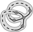
Figure 11. Example of a ribbon graph that does not embed into $\mathbb{R}^{2}$.

Proof.

Here we do not assume that the collection $\gamma$ is necessary maximal. When $\Gamma(S,\gamma)$ has a single vertex, then we prove the proposition using direct computation and the description of the boundary components corresponding to each possible ribbon graph. We refer to [MZ] for this description. Then our goal is to reduce ourselves to that case by removing successively from the collection $\gamma=\{\gamma_{1},\ldots,\gamma_{k}\}$ some $\gamma_{i}$ whose corresponding edges joins a vertex to a distinct one.

We define a new graph $G(S,\gamma)$, which is a deformation retract of the pure ribbon graph: the vertices of $G(S,\gamma)$ are the boundary components of each $S_{i}$, while the edges correspond to the saddle connections in $\gamma$ (see Figure 12). For each vertex, there is a cyclic order on the set of edges adjacent to the vertex consistent with the orientation of the plane. If the initial pure ribbon graph does not embed into the plane, then it is also the case for $G(S,\gamma)$. By construction, the Euler characteristic of $G(S,\gamma)$ is the same as the pure ribbon graph associated to $(S,\gamma)$, and is easier to compute.

Let $\Gamma(S,\gamma)$ contains at least two vertices. Choose a saddle connection representing an edge joining two distinct vertices of $\Gamma(S,\gamma)$, and up to renumeration, we can assume that this saddle connection is $\gamma_{1}$. Let us study the resulting configuration of $\gamma^{\prime}=\gamma\backslash\{\gamma_{1}\}$. The saddle connection $\gamma_{1}$ is on the boundary of two surfaces $S_{1}$ and $S_{2}$. Then the connected components of $S\backslash\gamma^{\prime}$ are the same as the connected component of $S\backslash\gamma$ except that the surfaces $S_{1}$ and $S_{2}$ are now glued along $\gamma_{1}$, and hence define a single surface $S_{1,2}$. The genus of $S_{1,2}$ (after gluing disks on its boundary) is $g_{1}+g_{2}$.

The graph $G(S,\gamma^{\prime})$ is obtained from $G(S,\gamma)$ by shrinking an edge that joins two different vertices, so these two graphs have the same Euler characteristic $\chi_{1}$.

Furthermore, if $\gamma_{1}$ was in a boundary component of $S_{1}$ (resp. $S_{2}$) defined by the ordered collection $(\gamma_{1},\gamma_{i_{1}},\dots,\gamma_{i_{s}})$ (resp. $(\gamma_{1},\gamma_{j_{1}},\dots,\gamma_{j_{t}})$). Then the cyclic order in the corresponding boundary component of $S_{1,2}$ is defined by $(\gamma_{i_{1}},\dots,\gamma_{i_{s}},\gamma_{j_{1}},\dots,\gamma_{j_{t}})$. Therefore $G(S,\gamma^{\prime})$ is obtained from $G(S,\gamma)$ by shrinking the edge corresponding to $\gamma_{1}$ and removing an isolated vertex that might appear (see Figure 12). It is clear that the difference $(\chi_{2}-n)$ between the Euler characteristic of $G(S,\gamma)$ and its number of connected component is constant under this procedure. One can also remark that if $G(S,\gamma)$ is connected and does not embed into the plane (case $1$ of the proposition), then this is also true for $G(S,\gamma^{\prime})$.

Forgetting successively these $\gamma_{i}$ will lead to the case when $\Gamma(S,\gamma)$ has a single vertex. At each steps of the removing procedure, the numbers $\chi_{1}$ and $\chi_{2}-n$ do not change, and the sum of the genera associated to the vertices does not change either. This concludes the proof.

∎

Figure 12. Removing successively some elements of a collection ($\gamma_{1},\gamma_{2},\gamma_{3})$.

References

- [AEZ] J. Athreya, A. Eskin, A.Zorich, Rectangular Billiards and volume of spaces of quadratic differentials, in progress.
- [EM] A. Eskin, H. Masur, Asymptotic formulas on flat surfaces, Ergodic Theory and Dynamical Systems, 21 (2) (2001), 443–478.
- [EMZ] A. Eskin, H. Masur, A. Zorich, Moduli spaces of Abelian differentials: the principal boundary, counting problems, and the Siegel-Veech constants, Publ. Math. Inst. Hautes Études Sci. 97 (2003),61–179.
- [HLM] P. Hubert, E. Lanneau, M. Möller, The Arnoux-Yoccoz Teichmüller disc, preprint 2006, arXiv:math/0611655v1 [math.GT].
- [HM] J. Hubbard, H. Masur, Quadratic differentials and foliations, Acta Math., 142 (1979), 221–274.
- [KaZe] A. Katok, A. Zemlyakov. Topological transitivity of billiards in polygons, Math. Notes, 18, (1975), 760-764.
- [KZ] M. Kontsevich, A. Zorich Connected components of the moduli spaces of Abelian differentials with prescribed singularities. Invent. Math. 153 (2003), no. 3, 631–678.
- [L1] E. Lanneau, Hyperelliptic components of the moduli spaces of quadratic differentials with prescribed singularities, Comment. Math. Helv. 79 (2004), no. 3, 471–501.
- [L2] E. Lanneau, Connected components of the strata of the moduli spaces of quadratic differentials Preprint 2004, arXiv:math/0506136v2 [math.GT].
- [M] H. Masur, Interval exchange transformations and measured foliations. Ann. of Math., 115 (1982), 169-200.
- [MS] H. Masur, J. Smillie, Hausdorff dimension of sets of nonergodic measured foliations. Ann. of Math. 134 (1991), 455–543.
- [MT] H. Masur, S. Tabachnikov, Rational billiards and flat structures. Handbook of dynamical systems, Vol. 1A, North-Holland, Amsterdam, (2002), 1015-1089.
- [MZ] H. Masur, A. Zorich, Multiple saddle connections on flat surfaces and the principal boundary of the moduli space of quadratic differentials, arXiv:math/0402197v2 [math.GT], to appear in GAFA.
- [Mc] C. McMullen, Dynamics of over moduli space in genus two. Ann. of Math., 165, 397-456 (2007).
- [V1] W.A. Veech, Gauss measures for transformations on the space of in- terval exchange maps. Ann. of Math., 115, 201-242 (1982).
- [V2] W.A. Veech, The Teichmüller geodesic flow. Ann. of Math., 124, 441-530 (1986).
- [Z] A. Zorich, Flat Surfaces. In collection “Frontiers in Number Theory, Physics and Geometry. Volume 1: On random matrices, zeta functions and dynamical systems”, P. Cartier; B. Julia; P. Moussa; P. Vanhove (Editors), Springer-Verlag, Berlin, (2006), 439-586.