Determining the Magnetic Field Orientation of Coronal Mass Ejections from Faraday Rotation

Abstract

We describe a method to measure the magnetic field orientation of coronal mass ejections (CMEs) using Faraday rotation (FR). Two basic FR profiles, Gaussian-shaped with a single polarity or “N”-like with polarity reversals, are produced by a radio source occulted by a moving flux rope depending on its orientation. These curves are consistent with the Helios observations, providing evidence for the flux-rope geometry of CMEs. Many background radio sources can map CMEs in FR onto the sky. We demonstrate with a simple flux rope that the magnetic field orientation and helicity of the flux rope can be determined 2-3 days before it reaches Earth, which is of crucial importance for space weather forecasting. An FR calculation based on global magnetohydrodynamic (MHD) simulations of CMEs in a background heliosphere shows that FR mapping can also resolve a CME geometry curved back to the Sun. We discuss implementation of the method using data from the Mileura Widefield Array (MWA).

1 Introduction

Coronal mass ejections (CMEs) are recognized as primary drivers of interplanetary disturbances. The ejected materials are often associated with large southward magnetic fields which can reconnect with geomagnetic fields and produce storms in the terrestrial environment (Dungey, 1961; Gosling et al., 1991). Determination of the CME magnetic field orientation is thus of crucial importance for space weather forecasting. However, nearly all atoms are ionized at the coronal temperature $\sim 2\times 10^{6}$ K, making it difficult to detect the coronal magnetic field through Zeeman splitting of spectral lines as is routinely done for the photospheric field. A typical way to estimate the coronal magnetic field above 2 $R_{\odot}$ ($R_{\odot}$ being the solar radius) is theoretical extrapolation using the photospheric fields as boundary conditions, which can only be checked by comparison to the field strength measured from radio bursts and the orientation determined from soft X-ray observations. The field orientation is also hard to infer from white-light coronagraph images. Spacecraft near the first Lagrangian point (L1) measure the local fields but can only give a warning time for arrival at Earth of $\sim 30$ minutes (Vogt et al., 2006; Weimer et al., 2002).

A possible method to measure the coronal magnetic field is Faraday rotation (FR), the rotation of the polarization plane of a radio wave as it traverses a magnetized plasma. The first FR experiment was conducted in 1968 by Pioneer 6 during its superior solar conjunction (Levy et al., 1969). The observed FR curve features a “W”-shaped profile over a time period of 2-3 hours with rotation angles up to 40^∘ from the quiescent baseline. This FR event was interpreted as a coronal streamer stalk of angular size 1-2^∘ (Woo, 1997), but Pätzold & Bird (1998) argue that the FR curve is produced by the passage of a series of CMEs. Joint coronagraph observations are needed to determine whether an FR transient is caused by CMEs. Subsequent FR observations by the Pioneer and Helios spacecraft reveal important information on the quiet coronal field (Stelzried et al., 1970; Pätzold et al., 1987) and magnetic fluctuations (Hollweg et al., 1982; Efimov et al., 1996; Andreev et al., 1997; Chashei et al., 1999, 2000). FR fluctuations are currently the only source of information for the coronal field fluctuations. Independent knowledge of the electron density, however, is needed in order to study the background field and fluctuations.

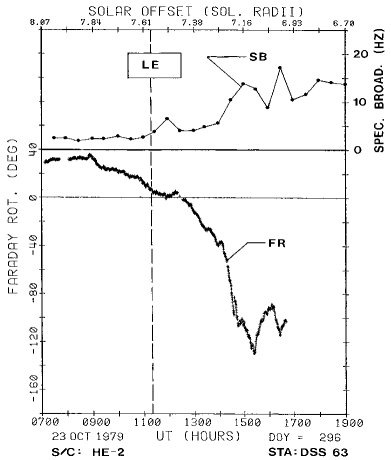
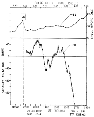
Figure 1: Time profiles of FR (bottom) and spectral broadening (top) of the Helios 2 signal during the CMEs of 23 October 1979 (left) and 24 October 1979 (right) recorded at the Madrid station DSS 63. The apparent solar offset of Helios 2 is given at the top. The dashed vertical line indicates the arrival time of the CME leading edge with uncertainties given by the width of the box “LE”. Large deviations in FR following the leading edge indicate the arrival of the CME’s bright core. Reproduced from Bird et al. (1985).

Joint coronagraph and FR measurements of CMEs were also conducted when the Helios spacecraft, with a downlink signal at a wavelength $\lambda=13$ cm, was occulted by CME plasma. Bird et al. (1985) establish a one-to-one correspondence between the SOLWIND white-light transients and FR disturbances for 5 CMEs. Figure 1 displays the time histories of FR and spectral broadening for two CMEs. Note that the spectral broadening is proportional to the plasma density fluctuations; the increased spectral broadening is consistent with the enhanced density fluctuations within CMEs and their sheath regions (Liu et al., 2006b). The FR through the 23 October 1979 CME shows a curve (note a data gap) which seems not to change sign during the CME passage; a single sign in FR indicates a monopolar magnetic field. The 24 October 1979 CME displays an FR curve which is roughly “N”-like across the zero rotation angle, indicative of a dipolar field. Other CMEs in the work of Bird et al. (1985) give similar FR curves, either an “N”-type or a waved shape around the zero level. Based on a simple slab model for CMEs, the mean transient field magnitude is estimated to be 10 - 100 mG scaled to $2.5R_{\odot}$, which seems larger than the mean background field. The CME field geometry, as implied by these FR curves, will be discussed below. These features demonstrate why radio occultation measurements are effective in detecting CMEs.

FR experiments using natural radio sources, such as pulsars and quasars, have also been performed. FR observations of this class were first conducted by Bird et al. (1980) during the solar occultation of a pulsar. The advantage of using natural radio sources is that many of these sources are present in the vicinity of the Sun and provide multiple lines of sight which can be simultaneously probed by a radio array. We can thus make a two-dimensional (2-D) mapping of the solar corona and the inner heliosphere with an extended distribution of background radio sources.

In this paper, we show a method to determine the magnetic field orientation of CMEs using FR. This method enables us to acquire the field orientation 2 - 3 days before CMEs reach Earth, which will greatly improve our ability to forecast space weather. The data needed to implement this technique will be available from the Mileura Widefield Array (MWA) (Salah et al., 2005). The magnetic structure obtained from MWA measurements with this method will fill the missing link in coronal observations of the CME magnetic field and also place strong constraints on CME initiation theories.

2 Modeling the Helios Observations

The FR technique uses the fact that a linearly polarized radio wave propagating through a magnetized plasma will undergo a rotation in its plane of polarization. The rotation angle is given by $\Omega=\lambda^{2}RM$, where $\lambda$ is the wavelength of the radio wave. The rotation measure, $RM$, is expressed as

$$RM=\frac{e^{3}}{8\pi^{2}\epsilon_{0}m_{e}^{2}c^{3}}\int n_{e}\textbf{B}\cdot d\textbf{s},$$ (1)

where $e$ is the electron charge, $\epsilon_{0}$ is the permittivity of free space, $m_{e}$ is the electron mass, $c$ is the speed of light, $n_{e}$ is the electron density, B is the magnetic field, and $d\textbf{s}$ is the vector incremental path defined to be positive toward the observer. FR responds to the magnetic field, making it a useful tool to probe the coronal transient and quiet magnetic fields. Note that the polarization vector may undergo several rotations across the coronal plasma. Measurements at several frequencies are needed to break the degeneracy; observations as a function of time can also help to trace the rotation through its cycles.

In situ observations of CMEs from interplanetary space indicate that CMEs are often threaded by magnetic fields in the form of a helical flux rope (Burlaga et al., 1981; Burlaga, 1988; Lepping et al., 1990). This helical structure either exists before the eruption (Chen, 1996; Kumar & Rust, 1996; Gibson & Low, 1998; Lin & Forbes, 2000), as needed for supporting prominence material, or is produced by magnetic reconnection during the eruption (e.g., Mikić & Linker, 1994). The flux rope configuration reproduces the white-light appearance of CMEs (Chen, 1996; Gibson & Low, 1998). This well-organized structure will display a specific FR signature easily discernible from the ambient medium, but direct proof of the flux-rope geometry of CMEs at the Sun has been lacking.

2.1 Force-Free Flux Ropes

Here we model the Helios observations using a cylindrically symmetric force-free flux rope (Lundquist, 1950) with

$$\textbf{B}=B_{0}J_{0}(\alpha r)\hat{z}+B_{0}HJ_{1}(\alpha r)\hat{\phi}$$ (2)

in axis-centered cylindrical coordinates $(\hat{r},\hat{\phi},\hat{z})$ in terms of the zeroth and first order Bessel functions $J_{0}$ and $J_{1}$ respectively, where $B_{0}$ is the field magnitude at the rope axis, $r$ is the radial distance from the axis, and $H$ specifies the left-handed (-1) or right-handed (+1) helicity. We take $\alpha r_{0}=2.405$, the first root of the $J_{0}$ function, so $\alpha$ determines the scale of the flux-rope radius $r_{0}$. The electron density is obtained by assuming a plasma beta $\beta=0.1$ and temperature $T=10^{5}$ K, as implied by the extrapolation of in situ measurements (e.g., Liu et al., 2005, 2006a). Combining equations (1) and (2) with a radio wave path gives the FR.

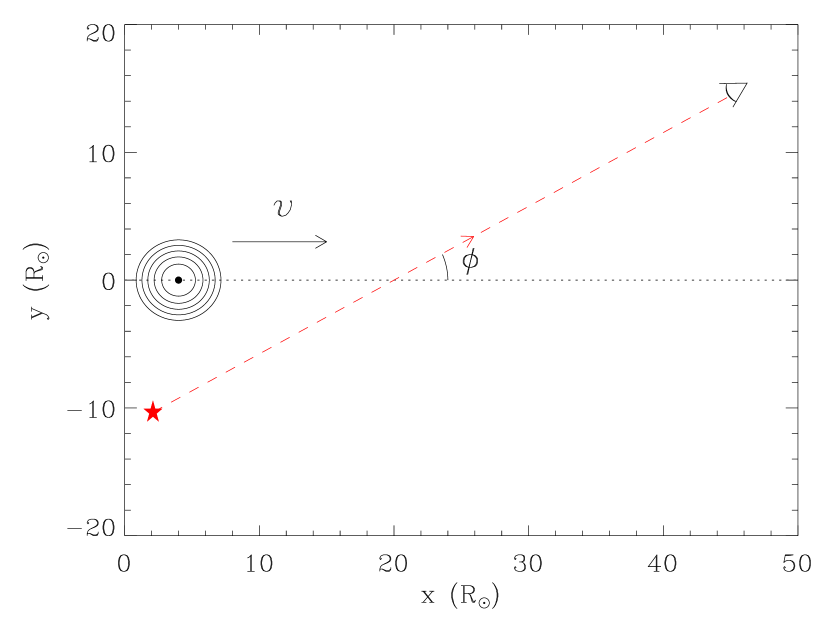
Figure 2: Schematic diagram of a force-free flux rope and the line of sight from a radio source to an observer projected onto the plane of the flux-rope cross section. The flux rope moves at a speed $v$ across the line of sight which makes an angle $\phi$ with the motion direction.

For simplicity, we consider a frame with the $x$-$y$ plane aligned with the flux-rope cross section at its center and the $z$ axis along the axial field. Figure 2 shows the diagram of the flux rope with the projected line of sight. The flux rope, initially at 4$R_{\odot}$ away from the Sun with a constant radius $r_{0}=3.6R_{\odot}$ and length 20$R_{\odot}$, moves with a speed $v=500$ km s^-1 in the $x$ direction across a radio ray path. The radio signal path makes an angle $\theta$ with respect to the plane and $\phi$ with the motion direction when projected onto the plane. The magnetic field strength at the rope axis is adopted to be $B_{0}=25$ mG, well within the range estimated from the Helios observations (Bird et al., 1985).

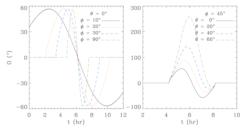
Figure 3: FR at $\lambda=13$ cm through the force-free flux rope as a function of time. Left is the rotation angle with $\theta$ fixed to 0^∘ and $\phi=[10^{\circ},20^{\circ},30^{\circ},90^{\circ}$], and right is the rotation angle with $\phi$ fixed to 45^∘ and $\theta=[0^{\circ},20^{\circ},40^{\circ},60^{\circ}$].

The resulting FR curves are displayed in Figure 3. A radio source occulted by the moving flux rope gives two basic types of FR curves, Gaussian-shaped and “N”-shaped (or inverted “N”) depending on the orientation of the radio wave path with respect to the flux rope. When the radio signal path is roughly along the flux rope (say, for $\phi=45^{\circ}$ and $\theta=60^{\circ}$ as shown in the right panel), the axial field overwhelms the azimuthal field along the signal path, so the FR curve would be Gaussian-like, indicative of a monopolar field. For a signal path generally perpendicular to the flux rope, the azimuthal field dominates and changes sign along the path, so the rotation curve would be “N” or inverted “N” shaped with a sign change (left panel), suggestive of a dipolar field. These basic curves are consistent with the Helios measurements. Two adjacent flux ropes with evolving fields could yield a “W”-shaped curve as observed by Pioneer 6 (Levy et al., 1969; Pätzold & Bird, 1998). The time scale and magnitude of the observed FR curves are also reproduced. When $\theta=0^{\circ}$, the line of sight is within the plane. Varying $\phi$ gives a variety of time scales of FR, ranging from $\sim 3$ to more than 10 hours, but the peak value of FR is fixed at $\sim 57^{\circ}$. These numbers are consistent with the Helios data shown in the right panel of Figure 1. When $\theta$ is close to $90^{\circ}$, the observer would be looking along the flux rope. The axial field produces a strong FR, but decreasing $\theta$ will diminish the rotation angle and make the curve more and more “N”-like. The time scale, however, remains at 4 hours. For $\phi=45^{\circ}$ and $\theta=40^{\circ}$, the rotation angle is up to $140^{\circ}$, in agreement with the Helios data shown in the left panel of Figure 1.

2.2 Non-Force-Free Flux Ropes

A non-force-free flux rope could give more flexibility in the field configuration. Consider a magnetic field that is uniform in the $z$ direction in terms of rectangular coordinates. Since $\nabla\cdot\textbf{B}=0$, the magnetic field can be expressed as

$${\bf B}=\left({\partial A\over\partial y},-{\partial A\over\partial x},B_{z}\right),$$ (3)

where the vector potential is defined as ${\bf A}=A(x,y)\hat{\bf z}$. The MHD equilibrium, ${\bf j}\times{\bf B}-\nabla p=0$, gives (e.g., Sturrock, 1994)

$${\partial^{2}A\over\partial x^{2}}+{\partial^{2}A\over\partial y^{2}}=-\mu_{0}{d\over dA}\left(p+{B_{z}^{2}\over 2\mu_{0}}\right)=-\mu_{0}j_{z},$$ (4)

where $\mu_{0}$ is the permeability of free space, $p$ is the plasma thermal pressure, and $j_{z}$ is the $z$ component of the current density. Equation (4) is known as the Grad-Shafranov equation. We see from this equation that $p$, $B_{z}$ and hence $j_{z}$ are a function of $A$ alone. A special form of this equation $\nabla^{2}\tilde{A}=\exp(-2\tilde{A})$ (in properly scaled units) has the solution (e.g., Schindler et al., 1973)

$$\tilde{A}=\ln\left[\alpha\cos\tilde{x}+\sqrt{1+\alpha^{2}}\cosh\tilde{y}\right].$$ (5)

This nonlinear solution has been called the periodic pinch since it has the form of a 2-D neutral sheet perturbed by a periodic chain of magnetic islands centered in the current sheet. Here $\tilde{A}$, $\tilde{x}$ and $\tilde{y}$ are dimensionless quantities, and $\alpha$ is a free parameter that can be used to control the aspect ratio of the magnetic islands.

From equations (3)-(5) we obtain

$$j_{z}=-\frac{B_{0}}{\mu_{0}L_{0}}\exp\left(\frac{-2A}{B_{0}L_{0}}\right),$$ (6)

$$B_{x}=B_{0}\frac{\sqrt{1+\alpha^{2}}\sinh(y/L_{0})}{\alpha\cos(x/L_{0})+\sqrt{1+\alpha^{2}}\cosh(y/L_{0})},$$ (7)

$$B_{y}=B_{0}\frac{\alpha\sin(x/L_{0})}{\alpha\cos(x/L_{0})+\sqrt{1+\alpha^{2}}\cosh(y/L_{0})},$$ (8)

where $B_{0}$ and $L_{0}$ are scales of the field magnitude and length, respectively. The axial field $B_{z}$ and the thermal pressure can be obtained from $\frac{d}{dA}(p+\frac{B_{z}^{2}}{2\mu_{0}})=j_{z}$, which gives

$$p+\frac{B_{z}^{2}}{2\mu_{0}}=\frac{B_{0}^{2}}{2\mu_{0}}\exp\left(\frac{-2A}{B_{0}L_{0}}\right)+\frac{B_{1}^{2}}{2\mu_{0}},$$

where $B_{1}$ is an arbitrary constant. Assuming a factor $\varepsilon$ in the partition of the total pressure, we have

$$p=\varepsilon\frac{B_{0}^{2}}{2\mu_{0}}\left[\left(\alpha\cos\frac{x}{L_{0}}+\sqrt{1+\alpha^{2}}\cosh\frac{y}{L_{0}}\right)^{-2}+\frac{B_{1}^{2}}{B_{0}^{2}}\right],$$ (9)

$$B_{z}=\pm\sqrt{1-\varepsilon}B_{0}\left[\left(\alpha\cos\frac{x}{L_{0}}+\sqrt{1+\alpha^{2}}\cosh\frac{y}{L_{0}}\right)^{-2}+\frac{B_{1}^{2}}{B_{0}^{2}}\right]^{1/2}.$$ (10)

Adjusting the parameters $\alpha$ and $\varepsilon$ gives a variety of flux rope configurations, circular and non-circular, force-free and non-force-free.

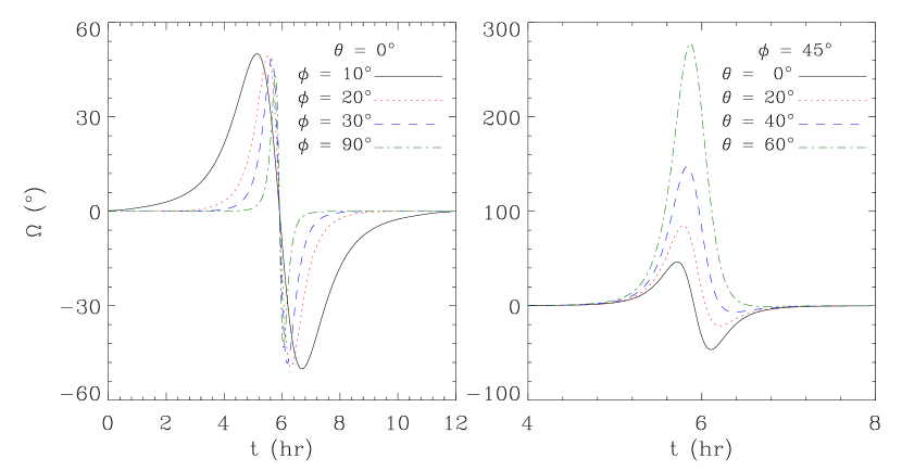
Figure 5: Same format as Figure 3, but for crossings of the non-force-free flux rope.

A flux rope of this kind is displayed in Figure 4. As can be seen, this flux rope lies within a current sheet. To single out the flux rope, we require $0\leq x\leq 2\pi L_{0}$ and $-\pi L_{0}/2\leq y\leq\pi L_{0}/2$ initially, where $L_{0}=1.5R_{\odot}$. The flux rope is still $20R_{\odot}$ long, moving with $v=500$ km s^-1 across the line of sight. Other parameters are assumed to be $B_{0}=10$ mG, $B_{1}=0$, $\alpha=2$, $\varepsilon=0.1$, and the temperature $T=10^{5}$ K. Figure 5 shows the calculated FR. These curves are generally similar to those for a cylindrically symmetric force-free flux rope. Unlike the force-free flux-rope counterpart, the FR curves show a smooth transition from the zero angle to peak values. In addition, they are narrower in width, which may result from fields and densities which are more concentrated close to the axis. Note that the field magnitude is $\sim 40$ mG at the axis of the non-force-free flux rope. These profiles can also qualitatively explain the Helios observations.

The above results suggest that CMEs at the Sun manifest as flux ropes, confirming what previously could only be inferred from in situ data (Burlaga, 1988; Lepping et al., 1990). They also reinforce the connection of CMEs observed by coronagraphs with magnetic clouds identified from in situ measurements.

3 2-D Mapping of CMEs

As demonstrated above, even a single radio signal path can give hints on the magnetic structure of CMEs. Ambiguities in the flux rope orientation cannot be removed based on only one radio ray path. The power of the FR technique lies in having multiple radio sources, especially when a 2-D mapping of CMEs onto the sky is possible.

3.1 A Single Flux Rope

For a flux-rope configuration, the magnetic field is azimuthal close to the rope edge and purely axial at the axis. The rotation measure would be positive through the part of the rope with fields coming toward an observer and negative through the part with fields leaving the observer, so the azimuthal field orientation can be easily recognized with data from multiple lines of sight (radio ray paths). A key role is played by the axial component, which tells us the helicity of the flux rope. Consider a force-free flux rope for simplicity. For points on a line parallel to the rope axis within the flux rope, the field direction as well as the magnitude is the same. The fields on this line would make different angles with a variety of radio signal paths since the signal path is always toward the observer. As long as the axial field component is strong enough, these different angles will lead to a gradient in the rotation measure along the rope.

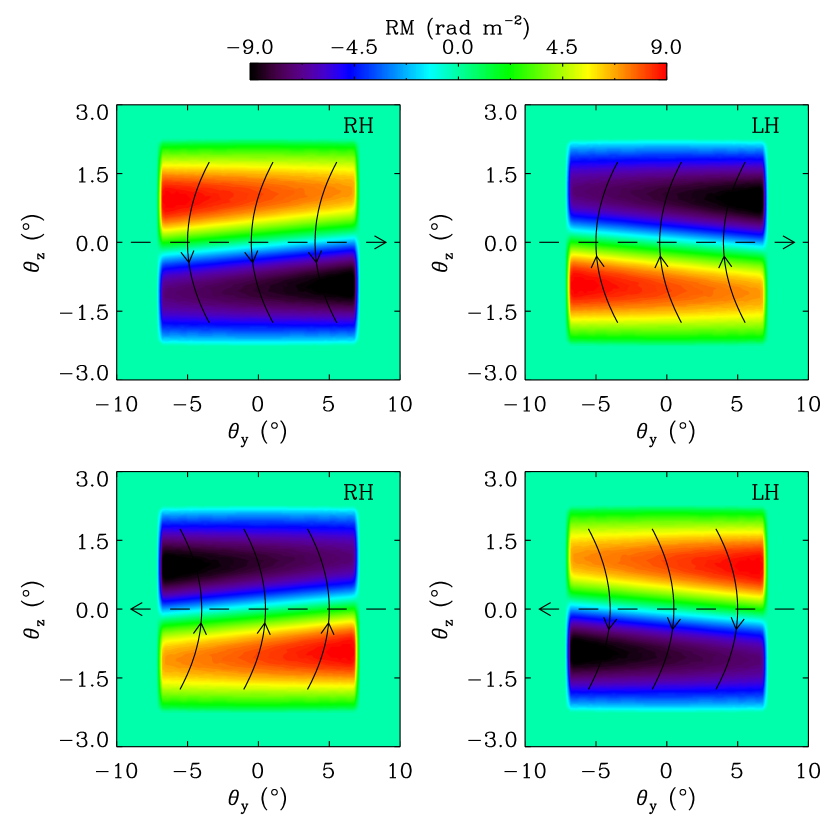
Figure 6: Mapping of the rotation measure corresponding to the four configurations of a flux rope onto the sky. The color shading indicates the value of the rotation measure. The arrows show the directions of the azimuthal and axial magnetic fields, from which a left-handed (LH) or right-handed (RH) helicity is apparent. Each configuration of the flux rope has a distinct rotation measure pattern.

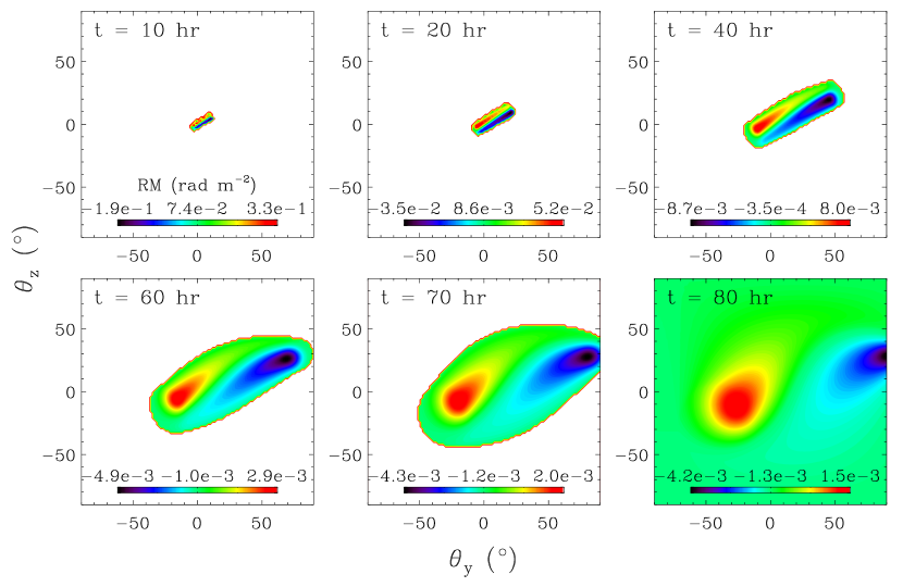
Figure 7: FR mapping of the whole sky at a resolution of $\sim 3.2$ degrees as a tilted flux rope moves away from the Sun. Note that the motion direction of the flux-rope center is not directly toward Earth. Values of the rotation measure for each panel are indicated by the color bar within the panel. Also shown is the time at the top for each snapshot.

Assuming an observer sitting at Earth, we calculate the FR pattern projected onto the sky for a force-free flux rope viewed from many radio sources. A flux rope has two possibilities for the axial field direction, with each one accompanied by either a left-handed or right-handed helicity. Plotted in Figure 6 are the four possible configurations as well as their rotation measure patterns. The angle $\theta_{y}$ defines the azimuthal angle of a line of sight with respect to the Sun-Earth (observer) direction in the solar ecliptic plane, while $\theta_{z}$ is the elevation angle of the line of sight with respect to the ecliptic plane. The flux rope, with axis in the ecliptic plane and perpendicular to the Sun-Earth direction, is centered at 10$R_{\odot}$ from the Sun and has a radius of $r_{0}=8R_{\odot}$ and length $50R_{\odot}$. The magnetic field magnitude is assumed to be 10 mG at the rope axis. The gradient effect in the rotation measure along the flux rope is apparent in Figure 6 and it produces a one-to-one correspondence between the flux-rope configuration and the rotation measure pattern. The four configurations of a flux rope can thus be uniquely determined from the global behavior of the rotation measure, which gives the axial field orientation and the helicity. In order to fully resolve the flux rope, we have assumed $\sim 80$ radio sources per square degree on the sky, but in practice a resolution of 250 times lower can give enough information for the field orientation and helicity (see Figure 7).

The FR mapping obtained from multiple radio sources can also help to determine the speed and orientation of CMEs as they move away from the Sun. This mapping is similar to coronagraph observations. While the polarized brightness (Thomson-scattered, polarized component of the coronal brightness) is sensitive to the electron density, FR reacts to the magnetic field as well as the electron density and thus may be able to track CMEs to a larger distance than white light imaging. Figure 7 gives snapshots at different times of a tilted flux rope moving outward from the Sun. A Sun-centered coordinate system is defined such that the $x$ axis extends from the Sun to Earth, the $z$ axis is normal to and northward from the solar ecliptic plane, and the $y$ axis lies in the ecliptic plane and completes the right handed set. A force-free flux rope, initially centered at (2, 2, 2)$R_{\odot}$ in this frame and oriented at 30^∘ from the ecliptic plane and 70^∘ from the Sun-Earth line, moves at a speed 500 km s^-1 from the Sun along the direction with elevation angle 10^∘ and azimuthal angle 20^∘. The flux rope evolution is constructed by assuming a power law dependence with distance $R$ (in units of AU) for the rope size and physical parameters, i.e.,

$$r_{0}=0.2\times R^{0.78}~{}{\rm AU}$$

for the rope radius,

$$B_{0}=15\times R^{-1.5}~{}{\rm nT}$$

for the field magnitude at the axis, and

$$T=3\times 10^{4}\times R^{-0.72}~{}{\rm K}$$

for the temperature. The rope length is kept at 3 times the rope diameter, and the plasma $\beta$ is kept at 0.1. Similar power-law dependences have been identified by a statistical study of CME evolution in the solar wind (Liu et al., 2005, 2006a), but note that the transverse size of the flux-rope cross section could be much larger than the radial width (Liu et al., 2006c).

The 2-D mapping has a pixel size of about 3.2 degrees. Even at such a low resolution, the flux rope can be recognized several hours after appearance at the Sun. The orientation of the flux rope with respect to the ecliptic plane is apparent in the first few snapshots, but note that this elevation angle may be falsified by the projection effect. The gradient effect in the rotation measure along the flux rope is discernable at 10 hours and becomes clearer around 20 hours. A right-handed helicity with axial fields skewed upward can be obtained from this gradient after a comparison with Figure 6 (top left). When the flux rope is closer to Earth, its appearance projected onto the sky becomes more and more deformed. Finally, when Earth is within the flux rope (around 80 hours), an observer would see two spots with opposite polarities produced by the ends of the flux rope.

Note that the above conclusions are not restricted to cylindrically symmetric force-free flux ropes. We have also used the non-force-free solutions of the steady state Vlasov-Maxwell equations (see §2.2), which unambiguously give the same picture. The FR technique takes advantage of an axial magnetic field coupled with the azimuthal component, which is the general geometry of a flux rope. This robust feature makes possible a precise determination of the CME field orientation. A curved flux rope with turbulent fields, however, may need caution in determining the axial field direction (see below).

3.2 MHD Simulations with Background Heliosphere

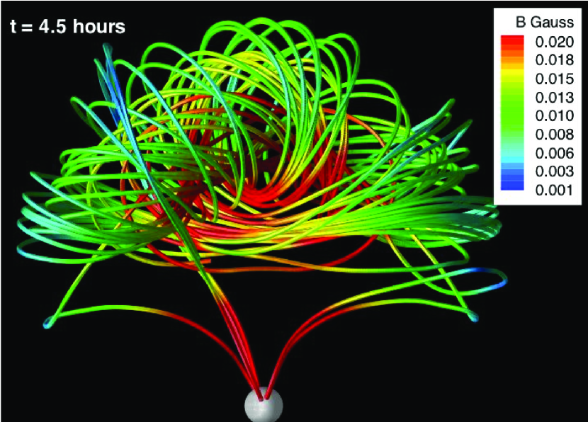
Figure 8: A 3-D rendering of the CME magnetic field lines at 4.5 hours after initiation. The color shading indicates the field magnitude and the white sphere represents the Sun.

The above FR calculation does not take into account the background heliosphere. In this sense, the 2-D mapping may be considered as a difference imaging between the transient and background heliospheres. Here we use for the FR calculation 3-D ideal MHD simulations of a CME propagating into a background heliosphere (Manchester et al., 2004). The simulations are performed using the so-called Block Adaptive Tree Solar-Wind Roe Upwind Scheme (BATS-R-US). A specific heating function is assumed to produce a global steady-state model of the corona that has high-latitude coronal holes (where fast winds come from) and a helmet streamer with a current sheet at the equator. A twisted flux rope with both ends anchored in the photosphere is then inserted into the helmet streamer. Removal of some plasma in the flux rope destabilizes the flux rope and launches a CME. The numerical simulation with adaptive mesh refinement captures the CME evolution from the solar corona to Earth. A 3-D view of the flux rope resulting from the simulations is displayed in Figure 8. The magnetic field, as represented by colored solid lines extending from the Sun, winds to form a helical structure within the simulated CME. The field has a strong toroidal (axial) component close to the axis but is nearly poloidal (azimuthal) at the surface of the rope.

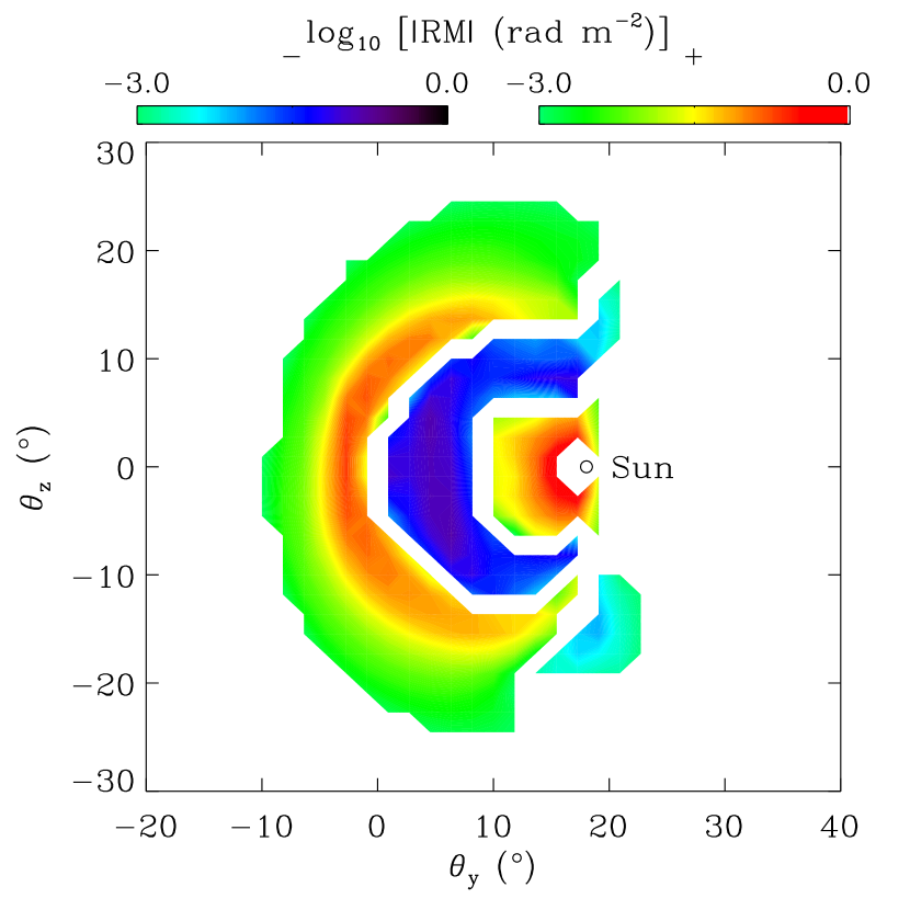
Figure 9: Mapping of the rotation measure difference between the MHD simulation at 24 hours and the steady state heliosphere. The two color bars indicate the logarithmic scale of the absolute value of the negative (-) and positive (+) rotation measure, respectively.

A fundamental problem in CME studies which remains to be resolved is whether CMEs are magnetically connected to the Sun as they propagate through interplanetary medium. Most theoretical modeling assumes a twisted flux rope with two ends anchored to the Sun (Chen, 1996; Kumar & Rust, 1996; Gibson & Low, 1998). This scenario is suggested by energetic particles of solar origin observed within a magnetic cloud (Kahler & Reames, 1991). An isolated plasmoid is also a possible structure for CMEs (Vandas et al., 1993a; Vandas, 1993b). The FR mapping is capable of removing this ambiguity in that it can easily capture a flux-rope geometry bent toward the Sun. To show this capability, we calculate the FR mapping of the simulated CME in a background heliosphere. The MHD model gives a time series of data cubes of $300R_{\odot}$ in length. We subtract the background from the rotation measure of the CME data to avoid possible effects brought about by the finite domain. Figure 9 shows the difference mapping of the rotation measure at a resolution of $\sim 3.2$ degrees when the CME propagates a day ($\sim 70R_{\odot}$) away from the Sun. The simulation data are rotated such that the observer (projected onto the origin) can see the flux rope curved to the Sun. The coordinates, $\theta_{y}$ and $\theta_{z}$, are defined with respect to the observer. A flux rope extending back to the Sun is apparent in the difference image. The outer arc with positive rotation measures is formed by the azimuthal magnetic field pointing to the observer while the inner arc with negative rotation measures originates from the field with the opposite polarity. The rotation measure difference is positive near the Sun, which is due to a pre-existing negative rotation measure that becomes less negative after the CME eruption.

A closer look at the image would also reveal asymmetric legs of the flux rope. This effect, indicative of a right-handed helicity, is created by the different view angles as described above. The nose of the flux rope does not show a clear gradient in the rotation measure because the view angles of this part are similar. In the case of the two legs directed to the observer, two spots with contrary magnetic polarities will be seen, so the curved geometry may also help to clarify the field helicity.

4 Summary and Discussion

We have presented a method to determine the magnetic field orientation of CMEs based on FR. Our FR calculations, either with a simple flux rope or global MHD modeling, demonstrate the exciting result that the CME field orientation can be obtained 2-3 days before CMEs arrive at Earth, substantially longer than the warning time achieved by local spacecraft measurements at L1.

The FR curves through the CME plasma observed by Helios can be reproduced by a flux rope moving across a radio signal path. Two basic FR profiles, Gaussian-shaped with a single polarity or “N”-like with polarity reversals, indicate the orientation of the flux rope with respect to the signal path. Force-free and non-force-free flux ropes generally give the same picture, except some trivial differences reflecting the field and density distributions within a flux rope. The FR calculation with a radio signal path, combined with the Helios observations, shows that CMEs at the Sun appear as flux ropes.

2-D FR mapping of a flux rope using many radio sources gives the field orientation as well as the helicity. The orientation of azimuthal fields can be readily obtained since they yield rotation measures with opposite polarities. The axial component of the magnetic field creates a gradient in rotation measure along the flux rope, with which the flux rope configurations can be disentangled. Time-dependent FR mapping is also calculated for a tilted flux rope propagating away from the Sun. The orientation of the flux rope as a whole and its projected speed onto the sky can be determined from the snapshots of the flux rope mapped in FR. We further compute the FR mapping for a curved flux rope moving into a background heliosphere obtained from 3-D ideal MHD simulations. It is shown that the FR mapping can resolve a CME curved back to the Sun in addition to the field orientation. Difference imaging is needed to remove the FR contribution from the background medium.

The global FR map is a new technique for measuring the CME magnetic field. This method can determine the magnetic field orientation of CMEs without knowledge of the electron density. The electron density could be inferred from Thomson scattering measurements made by the SECCHI instrument (suite of wide angle coronagraphs) on STEREO which has stereoscopic fields of view (Howard, 2000). With the joint measurements of the electron density, the magnetic field strength can be estimated.

Note that the above results are a first-order attempt to predict what may be seen in FR. An actual CME likely shows a turbulent behavior and may have multiple structures along the line of sight; the rotation measure, an integral quantity along the line of sight, could display similar signatures for different structures. Therefore, interpretation of the FR measurements will be more complex than suggested here. However, having an instantaneous, global map of the rotation measure that evolves in time will be vastly superior to a time profile along a single line of sight, and comparison with coronagraph observations and actual measures of geoeffectiveness (e.g., the $D_{st}$ index) for a series of real events will eventually lead to the predictive capability proposed in this paper.

The present results also pave the way for interpreting future FR observations of CMEs by large radio arrays, particularly those operating at low frequencies (Oberoi & Kasper, 2004; Salah et al., 2005). The MWA - Low Frequency Demonstrator, specially designed for this purpose at 80-300 MHz, will feature wide fields of view, high sensitivity and multi-beaming capabilities (Salah et al., 2005). This array will be installed in Western Australia (26.4^∘S, 117.3^∘E), a radio quiet region. It will spread out $\sim 1.5$ km in diameter, achieving $\sim 8000$ m² of collecting area at 150 MHz and a field of view from 15^∘ at 300 MHz to 50^∘ at 80 MHz. The point source sensitivity will be about 20 mJy for an integration time of 1 s. The array is expected to monitor $\sim 300$ background radio sources within 13^∘ elongation ($\sim 50R_{\odot}$) from the Sun, providing a sufficient spatial sampling of the inner heliosphere. In addition, this array will be able to capture a rotation measure of $\sim 10^{-2}$ rad m^-2 and thus is remarkably sensitive to the magnetic field. Science operations of the array will start in 2009. Implementation of our method by such an array would imply a coming era when the impact of the solar storm on Earth can be predicted with small ambiguities. It could also fill the missing link in coronal observations of the CME magnetic field, thus providing strong constraints on CME initiation theories.

Figure 4: Same format as Figure 2, but for a non-force-free flux rope embedded in a current sheet.

References

- Andreev et al. (1997) Andreev, V. E., Efimov, A. I., Samoznaev, L. N., Chashei, I. V., & Bird, M. K. 1997, Sol. Phys., 176, 387
- Bird et al. (1980) Bird, M. K., Schrüfer, E., Volland, H., & Sieber, W. 1980, Nature, 283, 459
- Bird et al. (1985) Bird, M. K., et al. 1985, Sol. Phys., 98, 341
- Burlaga et al. (1981) Burlaga, L. F., Sittler, E., Mariani, F., & Schwenn, R. 1981, J. Geophys. Res., 86, 6673
- Burlaga (1988) Burlaga, L. F. 1988, J. Geophys. Res., 93, 7217
- Chashei et al. (1999) Chashei, I. V., Bird, M. K., Efimov, A. I., Andreev, V. E., & Samoznaev, L. N. 1999, Sol. Phys., 189, 399
- Chashei et al. (2000) Chashei, I. V., Efimov, A. I., Samoznaev, L. N., Bird, M. K., & Pätzold, M. 2000, Adv. Space Res., 25, 1973
- Chen (1996) Chen, J. 1996, J. Geophys. Res., 101, 27499
- Dungey (1961) Dungey, J. W. 1961, Phys. Rev. Lett., 6, 47
- Efimov et al. (1996) Efimov, A. I., Bird, M. K., Andreev, V. E., & Samoznaev, L. N. 1996, Astron. Lett., 22, 785
- Gibson & Low (1998) Gibson, S. E., & Low, B. C. 1998, ApJ, 493, 460
- Gosling et al. (1991) Gosling, J. T., McComas, D. J., Philips, J. L., & Bame, S. J. 1991, J. Geophys. Res., 96, 7831
- Hollweg et al. (1982) Hollweg, J. V., et al. 1982, J. Geophys. Res., 87, 1
- Howard (2000) Howard, R. A., Moses, J. D., & Socker, D. G. 2000, Proc. SPIE, 4139, 259
- Kahler & Reames (1991) Kahler, S. W., & Reames, D. V. 1991, J. Geophys. Res., 96, 9419
- Kumar & Rust (1996) Kumar, A., & Rust, D. 1996, J. Geophys. Res., 101, 15667
- Lepping et al. (1990) Lepping, R. P., Jones, J. A., & Burlaga, L. F. 1990, J. Geophys. Res., 95, 11957
- Levy et al. (1969) Levy, G. S., et al. 1969, Science, 166, 596
- Lin & Forbes (2000) Lin, J., & Forbes, T. G. 2000, J. Geophys. Res., 105, 2375
- Liu et al. (2005) Liu, Y., Richardson, J. D., & Belcher, J. W. 2005, Plan. Space Sci., 53, 3
- Liu et al. (2006a) Liu, Y., Richardson, J. D., Belcher, J. W., Kasper, J. C., & Elliott, H. A. 2006a, J. Geophys. Res., 111, A01102, doi:10.1029/2005JA011329
- Liu et al. (2006b) Liu, Y., Richardson, J. D., Belcher, J. W., Kasper, J. C., & Skoug, R. M. 2006b, J. Geophys. Res., 111, A09108, doi:10.1029/2006JA011723
- Liu et al. (2006c) Liu, Y., et al. 2006c, J. Geophys. Res., 111, A12S03, doi:10.1029/2006JA011890
- Lundquist (1950) Lundquist, S. 1950, Ark. Fys., 2, 361
- Manchester et al. (2004) Manchester IV, W. B., et al. 2004, J. Geophys. Res., 109, A02107
- Mikić & Linker (1994) Mikić, Z., & Linker, J. A. 1994, ApJ, 430, 898
- Oberoi & Kasper (2004) Oberoi, D., & Kasper, J. C. 2004, Plan. Space Sci., 52, 1415
- Pätzold et al. (1987) Pätzold, M., et al. 1987, Sol. Phys., 109, 91
- Pätzold & Bird (1998) Pätzold, M., & Bird, M. K. 1998, Geophys. Res. Lett., 25, 2105
- Salah et al. (2005) Salah, J. E., et al. 2005, Proc. SPIE, 5901, 124
- Schindler et al. (1973) Schindler, K., Pfirsch, D., & Wobig, H. 1973, Plasma Phys., 15, 1165
- Stelzried et al. (1970) Stelzried, C. T., et al. 1970, Sol. Phys., 14, 440
- Sturrock (1994) Sturrock, P. A. 1994, Plasma Physics: An Introduction to the Theory of Astrophysical, Geophysical and Laboratory Plasmas (New York: Cambridge Univ. Press), 209
- Vandas et al. (1993a) Vandas, M., Fischer, S., Pelant, P., & Geranios, A. 1993a, J. Geophys. Res., 98, 11467
- Vandas (1993b) Vandas, M., Fischer, S., Pelant, P., & Geranios, A. 1993b, J. Geophys. Res., 98, 21061
- Vogt et al. (2006) Vogt, M. F., et al. 2006, Space Wea., 4, S09001
- Weimer et al. (2002) Weimer, D. R., et al. 2002, J. Geophys. Res., 107, A81210
- Woo (1997) Woo, R. 1997, Geophys. Res. Lett., 24, 97