Combustion waves in a model with chain branching reaction and their stability

Abstract

In this paper the travelling wave solutions in the adiabatic model with two-step chain branching reaction mechanism are investigated both numerically and analytically in the limit of equal diffusivity of reactant, radicals and heat. The properties of these solutions and their stability are investigated in detail. The behaviour of combustion waves are demonstrated to have similarities with the properties of nonadiabatic one-step combustion waves in that there is a residual amount of fuel left behind the travelling waves and the solutions can exhibit extinction. The difference between the nonadiabatic one-step and adiabatic two-step models is found in the behaviour of the combustion waves near the extinction condition. It is shown that the flame velocity drops down to zero and a standing combustion wave is formed as the extinction condition is reached. Prospects of further work are also discussed.

Keywords: combustion waves, Evans function, chain-branching reaction, linear stability, extinction

2000 Mathematics Subject Classification codes: 35K57, 80A25

1 Introduction

Combustion waves have been studied for some time and are topic of a relatively recent review [1]. They have been observed in numerous experiments [1] and play an important role in industrial processes, such as the production of advanced materials using Self-propagating High-temperature Synthesis (SHS) [2]. The one-step irreversible reaction models have contributed greatly to our understanding of these phenomena. In these models it is assumed that the reaction is well modeled by a single step of fuel ($F$) and oxidant ($O_{2}$) combining to produce products ($P$) and heat. The generic kinetic schemes of models with one-step chemistry are: $F\longrightarrow P+heat$ or $F+O_{2}\longrightarrow 2P+heat$, where the temperature dependent rate of the reaction is given by Arrhenius kinetics $k(T)=e^{-T_{a}/T}$ and $T_{a}$ is the activation temperature. These models have proven their usefulness since they are relatively simple and allow analytical investigation using asymptotic methods in the limit of infinitely large activation temperature [3, 4]. The most important feature of one-step models is that they have led to many useful and qualitatively correct predictions for phenomena such as: ignition, extinction and stability of diffusion flames; propagation and stability of premixed flames; flame balls and their stability; structure and propagation of flame edges etc.

However, in the overwhelming majority of cases, the chemical reactions in flames proceed according to a complex mechanism, that involves a variety of different steps [3]. Moreover, for many reactions, models with simple one-step kinetics may lead to erroneous conclusions as noted in [5]. In other words, if we want to obtain a realistic description of the flame kinetics, several different steps, each with its own intermediate chemical species, have to be taken into account. Recent advances in computational power have made it possible to study the flame behaviour using full numerical solutions of the equations of energy and mass transfer for all of the species involved with detailed chemistry. Several numerical codes have been developed in order to carry out these calculations, such as Sandia s CHEMKIN code [6] or the Flame Master code [7]. These numerical algorithms have been successfully applied to analyze the properties of both diffusion [8] and premixed flames [9]. Although such investigations are useful in providing some quantitative prediction for observed phenomena, there is still a great deal of uncertainty about the reliability of these complex models when applied to the prediction of generic behaviour of flames such as stable combustion regimes, limits of the flame extinction and particularly the onset of combustion phenomena such as pulsating and cellular combustion, when the reactions begin to change rapidly in space and/or time.

A logical compromise between the models with singe-step and detailed multi-step kinetics have been found recently in using reduced kinetic mechanisms. In a number of papers [8, 9, 10, 11] (listing only few of them) the detailed schemes of the hydrogen and methane oxidation, which include dozens of intermediate reactions, were successfully reduced to several steps. The remarkable feature of these type of models is that they allow on one hand, analytical investigation [10, 11] to be successfully undertaken, while on the other hand they are able to produce excellent quantitative results [8, 9] to accurately predict the main flame characteristics for some specific reactions such as flame propagation velocities, flame structures including the profiles of temperature and reactants etc. These studies are very important for applied problems, in which the properties of flames for specific reaction and flame configuration are studied.

The importance of investigation of flames with complex kinetics is well acknowledged in combustion literature and as noted in Clavin et al. [12] “a crucial first step in such a study consists in determining reduced schemes that capture the essence of complete network”. A particulary promising candidate is a two-step reaction mechanism. In this paper we only consider combustion waves in premixed flames. For premixed flames, several models involving two chemical steps have been considered previously. These studies address the fundamental (generic) properties of flames with multi-step reaction mechanisms rather than consider some specific combustion reaction. The two-step reactions can be split into two groups: reactions with competing steps [3, 12] and sequential steps [3, 13, 14, 15, 16, 17, 18]. In the first group of models three types of reactions are considered: (i) simple competing scheme $\bf C_{1}$: $A\rightarrow P_{1}$, $A\rightarrow P_{2}$; (ii) competing chain reaction scheme $\bf C_{2}$: $A\rightarrow B$, $A+B\rightarrow P$; (iii) competing chain branching scheme $\bf C_{3}$: $A+B\rightarrow 2B$, $A+B\rightarrow P$, where $A$ is the reactant, $B$ the radical, $P$ the product. The second group of the reactions includes several schemes: (i) non competitive reactions $\bf N_{1}$: [16] $A_{1}\rightarrow P_{1}$, $A_{2}\rightarrow P_{2}$; (ii) sequential fuel decomposition reaction $\bf N_{2}$: [3, 14, 17] $A\rightarrow B\rightarrow P$; (iii) chain branching reaction $\bf N_{3}$: [3, 13, 14, 15, 18] $A+B\rightarrow 2B$, $nB+M\rightarrow nP+M$, where $n=1$ in [14, 15] and $n=2$ in [3, 13] and $M$ is a third body. These schemes were investigated either analytically by using high activation energy asymptotic or numerically. As a rule the asymptotic methods allow the investigation only in certain distinguished limits when the inner equations arising in the asymptotic procedure can be integrated analytically [12, 14, 15, 17]. However, generally these equations cannot be integrated analytically due to the increased complexity of the two-step models in comparison to one-step reaction models and the inner equations are solved numerically to match them to the outer equation solutions [11, 12, 13]. In most cases the two-step reaction models show more rich dynamical behaviour in comparison to their single step counterparts. For given parameter values there can exist combustion wave solution branches travelling with unique speed, with two different speeds (C-shaped dependence of speed on parameters), and with three different speeds (S-shaped dependence of speed on parameters). The multiplicity of the flames suggests that a more complex stability behaviour also exist. However, the stability analysis of these flames are reported in only a few papers [12, 15] and has not been investigated systematically. Since the behaviour of multi-step models can differ from their one-step prototypes, we can expect a number of new phenomena such as bistability (which cannot be predicted by the one-step models) to be found as a result of such an analysis [12].

In this paper we focus on the investigation of premixed combustion waves in a model with non-competing two-step chain branching reaction. As noted in [14] the chain branching reaction is more realistic in describing real flames such as hydrocarbon flames in comparison to other two-step reaction models. This model was initially considered in [3] and then generalized in [13]. It is usually referred to as Zeldovich-Liñán model. In [13] the model is considered in a limiting case when the recombination step is fast in comparison to heat conduction time. Firstly,the resulting problem is investigated semi-analytically by using activation energy asymptotic first which provides a set of equations for the inner problem. These equations were then solved numerically. It was shown that there exists a unique travelling wave solution for given parameter values. In [11] a reduced two-step chain branching reaction for oxidation of hydrogen was studied. The methodology used in this paper is similar to [13] (i.e. semi-analytical investigation using activation energy asymptotics and numerical integration of the resulting equations). It was shown that the flame has a unique burning velocity. The results obtained in this paper are shown to be in a good agreement with numerical experiments for the detailed kinetic mechanism of the reaction, which indicates that the two-step reaction models might have a capacity of quantitatively predicting the flame behaviour. There are other papers devoted to investigation of the premixed flames in this model and we refer the reader to [15] for more detailed overview, however the stability of combustion waves in the Zeldovich-Liñán model has not been investigated. In [14, 15] a simplified version of Zeldovich-Liñán model is introduced. In this model the order of the recombination reaction is taken as $n=1$. In contrast to [3] the model also includes the linear heat loss to the surroundings. The model is studied in the limit of high activation energy which allows asymptotic analysis to be carried out successfully. The speed of the combustion wave is determined as a function of the parameters of the problem. It is shown that in the nonadiabatic case the dependence is C-shaped. For the adiabatic case the expression derived in [15] suggests a unique speed of the flame propagation. It is remarkable that in [15] the stability analysis of combustion waves is carried out for the case of the reactant Lewis number less than one. The analysis predicts that the wave can lose stability due to the cellular instabilities emerged in this case. In our previous paper [20] we have investigated the properties of the model introduced in [15] in the adiabatic case and in the limit of equal diffusivity of the reactant, the radical and heat. In contrast to [15] the activation energy in [20] is taken to be an arbitrary number (not an infinite number) and we used a different nondimensionalization. Our non dimensional parameters are common for one-step models, which makes for an easier comparison between the two models. In [20] the properties of the travelling wave solutions are investigated in detail by means of numerical simulation. It is demonstrated that the speed of combustion wave as a function of parameters is single valued. We have found that for finite activation energy there is a residual amount of reactant left behind the travelling combustion wave which is not used in the reaction. This makes the problem similar to the nonadiabatic one-step premixed flames. The other fact about the model considered in [20] which makes the similarity between the adiabatic two-step reaction and the nonadiabatic one-step system even stronger is that, at certain parameter values the combustion wave exhibits the extinction. However, it occurs in such manner that the speed of the wave drops to zero. This mainly distinguishes the one- and two-step models, since in the former case the wave can propagate for any parameter values and even in the nonadiabatic case the speed of combustion wave does not vanish for finite parameter values, whereas this is not the case for the two-step models.

Extinction of the combustion wave is a critical property of the model that also distinguished the two-step models form their one-step counterparts. Therefore we have also examined this property in detail in this paper. The other important question which will be studied here is the stability of the combustion wave. We will compare our results (where possible) with the predictions of the asymptotic analysis of [15]. In [20] the existence of multiple travelling wave train solutions is reported for some parameter values. Our analysis shows that besides wave trains, the solutions with various structure can also exist such as pulses, fronts with step-like structure etc. The properties and relevance of these solutions lies beyond the scope of this paper and will be discussed in future work. In this paper we will only consider the classical travelling front solutions.

The rest of the paper is organized as follows. The nondimensional model equations are introduced in section 2, and where possible, we have referred the reader to [20] to avoid repetition. In this section we also outline the formulation of the problem to obtain the travelling front solution and determine the condition for the existence of the travelling waves. Section 3 is devoted to the investigation of the travelling wave solution. In the first part of section 3, we summarize the properties of this solution which were obtained in [20]. We then determine the extinction limit for the travelling front solution. We analyze its behavior near the point of extinction using the matched asymptotic expansion method and compare the predictions of analytical and numerical approaches. We conclude section 3 by undertaking the stability analysis of the travelling wave solutions. Finally, in section 4 the concluding remarks are presented with some discussion for future work.

2 Model

We consider an adiabatic model (in one spatial dimension) that includes two steps: autocatalytic chain branching $A+B\rightarrow 2B$ and recombination $B+M\rightarrow C+M$. Here $A$ is the fuel, $B$ the radical, $C$ the product, and $M$ a third body. Following [3, 14, 15] we assume that all the heat of the reaction is released during the recombination stage and the chain branching stage does not produce or consume any heat. As noted in [3], in this scheme the recombination stage serves both as an inhibitor which terminates the chain branching and an accelerant which produces heat. According to [20], the equations governing this process can be written in nondimensional form as

$$\begin{array}[]{ccl}u_{t}&=&u_{xx}+rw,\\ v_{t}&=&\tau_{A}v_{xx}-\beta vwe^{-1/u},\\ w_{t}&=&\tau_{B}w_{xx}+\beta vwe^{-1/u}-r\beta w,\end{array}$$ (1)

where $u$, $v$ and $w$ are the non-dimensional temperature, concentration of fuel and radicals respectively; $x$ and $t$ are the dimensionless spatial coordinate and time respectively. In (1) the following non-dimensional parameters have been introduced: $\beta=c_{p}E/QR$, $r=A_{r}/A_{B}$, $\tau_{A,B}=\rho c_{p}D_{A,B}/k$, where $c_{p}$ is the specific heat; $D_{A}$ and $D_{B}$ represent the diffusivity of fuel and radicals respectively, $A_{r}$ and $A_{B}$ are constants of recombination and chain branching reactions respectively; $Q$ is the heat of the recombination reaction; $E$ is the activation energy for chain branching reaction; $R$ is the universal gas constant. Here parameter $\beta$ is the dimensionless activation energy of the chain-branching step which coincides with the corresponding definition for the one step model [4]. Parameter $r$ is the ratio of the characteristic time of the recombination and branching steps and cannot be reproduced in one step approximation of the flame kinetics.

Equations (1) are considered subject to the boundary conditions

$$\begin{array}[]{lllllllll}u=0,&&v=1,&&w=0&&\text{for}&&x\rightarrow\infty,\\ u_{x}=0,&&v_{x}=0,&&w=0&&\text{for}&&x\rightarrow-\infty.\end{array}$$ (2)

On the right boundary we have cold ($u=0$) and unburned state ($v=1$), where the fuel has not been consumed yet and no radicals have been produced ($w=0$). We also take the ambient temperature to be equal to zero. As noted in [19] this is a convenient way to circumvent the so-called “cold-boundary problem” and it does not change the generic behaviour of the system. On the left boundary ($x\rightarrow-\infty$) neither the temperature of the mixture nor the concentration of fuel can be specified. We only require that there is no reaction occurring so the solution reaches a stationary point of (1). Therefore the derivatives of $u$, $v$ are zeros and $w=0$ for $x\rightarrow-\infty$.

2.1 Travelling wave solution

We seek a solution to the problem (1), (2) in the form of a travelling wave $u(x,t)=u(\xi)$, $v(x,t)=v(\xi)$, and $w(x,t)=w(\xi)$, where we have introduced $\xi=x-ct$, a coordinate in the moving frame and $c$, the speed of the travelling wave. Substituting the travelling wave solution into the governing equations we obtain

$$\begin{array}[]{l}u_{\xi\xi}+cu_{\xi}+rw=0,\\ \tau_{A}v_{\xi\xi}+cv_{\xi}-\beta vwe^{-1/u}=0,\\ \tau_{B}w_{\xi\xi}+cw_{\xi}+\beta vwe^{-1/u}-r\beta w=0,\end{array}$$ (3)

and boundary conditions

$$\begin{array}[]{lllllllll}u=0,&&v=1,&&w=0&&\text{for}&&\xi\rightarrow\infty,\\ u_{\xi}=0,&&v_{\xi}=0,&&w=0&&\text{for}&&\xi\rightarrow-\infty.\end{array}$$ (4)

Following [3, 16] we consider the case when Lewis numbers for the fuel and the radicals are equal to unity. Although this assumption simplifies the problem significantly, it still allows the investigation of the generic properties of the system (3) and (4).

In the case $\tau_{A}=\tau_{B}=1$ equations (3) possess an integral $S=\beta u+v+w$. Using $S$ and the first boundary condition in (4), equations (3) can be reduced to a system of two second order equations for temperature and fuel concentration

$$\begin{array}[]{l}u_{\xi\xi}+cu_{\xi}+r(1-\beta u-v)=0,\\ v_{\xi\xi}+cv_{\xi}-\beta v(1-\beta u-v)e^{-1/u}=0.\end{array}$$ (5)

On the right boundary we require that $u=0$ and $v=1$, whereas on the left boundary ($\xi\rightarrow-\infty$) we modify the boundary conditions as follows

$$\begin{array}[]{ccc}u=\beta^{-1}(1-\sigma),&&v=\sigma,\end{array}$$ (6)

where $\sigma$ denotes the residual amount of fuel left behind the wave and is unknown until a solution is obtained. We note here that at first glance, system (5) looks very similar to the equations describing the dynamics of the one-step adiabatic reaction model considered in [19]. However, in contrast to the one-step adiabatic case, equations (5) do not have an integral which enabled further simplification in [19]. Moreover, boundary conditions (6) suggest that there can be some fuel left behind the reaction zone, which is impossible in the case of a one-step adiabatic reaction model.

2.2 Existence of the travelling wave solution

The basic properties of the system (5) can be found from the stability analysis of the fixed points on $\xi\rightarrow\pm\infty$. On the right hand side, as $\xi\rightarrow\infty$, the fixed point coordinates (or asymptotic values of $u$ and $v$) are given as $u=0$ and $v=1$. We will refer to this stationary point as the end point. The linearization of (5) around these values suggests that the end point is a saddle-node for all physical parameter values with corresponding eigenvalues given as $\mu_{1}=0$, $\mu_{2}=-c$, $\mu_{3,4}=(-c\pm\sqrt{c^{2}+4r\beta})/2$.

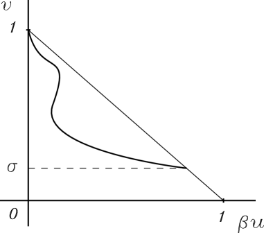
Figure 1: Schematic representation of the travelling wave solution on $(\beta u,v)$ plane.

In the opposite limit $\xi\rightarrow-\infty$, the fixed point (referred to as the starting point) has coordinates given by (6), i.e. any point lying on a line $v=1-\beta u$ in $(u,~{}v)$ plane can be a fixed point (or correspondingly, asymptotic values of temperature $u$ and fuel concentration $v$ belong to this line in the $(u,~{}v)$ plane as $\xi\rightarrow-\infty$). On the $(\beta u,~{}v)$ plane a travelling wave solution can be schematically represented as shown in figure 1. The linearization of the governing equations (5) around the values (6) suggests that the starting point can be either a saddle-node or a stable node depending on the parameter values. Namely, the eigenvalues of the linearized problem can be written in this case as: $\mu_{1}=0$, $\mu_{2}=-c$, $\mu_{3,4}=(-c\pm\sqrt{c^{2}+4\beta(r-\sigma e^{-\beta/(1-\sigma)})})/2$. The starting point is a saddle-node for $r>\sigma e^{-\beta/(1-\sigma)}$ and a stable node for $r<\sigma e^{-\beta/(1-\sigma)}$. In the latter case it is impossible to connect the starting point (as $\xi\rightarrow-\infty$) with the end point (as $\xi\rightarrow\infty$) with a trajectory in the phase space and therefore the solution does not exist. The condition

$$r=\sigma\exp{\displaystyle\frac{-\beta}{1-\sigma}}$$ (7)

defines a surface in the $(r,~{}\beta,~{}\sigma)$ parameter space which represents the boundary between the region, where the solution exists from the region where it does not. If any of the solution branches crosses this surface it has to exhibit extinction. Therefore, we can also refer (7) as the extinction condition. In figure 2, the boundary between the parameter regions where the travelling solutions exist (above the surface) or cease to exist (below the surface) is shown. The physical meaning of this condition can also be explained if we return to equation (1) and neglect the diffusion terms. Behind the travelling wave there has to be a stable state defined by (6) and $w=0$, where no radicals can be produced if some small variation of radical concentration is imposed. As seen from (1), the latter condition is satisfied if $r>\sigma\exp{\frac{-\beta}{1-\sigma}}$ and the right hand side of the last equation in (1) is not positive.

Figure 2: The extinction condition (7) plotted as a surface in the parameter space $(r,~{}\beta,~{}\sigma)$.

It is useful to consider several cross sections of (7) with the planes $r=constant$, since we will be studying the properties of the solutions to (5) for fixed values of $r$. The corresponding level curves are shown in figure 3 and are given as $\beta_{e}(\sigma)=(1-\sigma)\ln(\sigma/r)$. It is seen that $\beta$ as a function of $\sigma$ has a single maximum, $\beta_{m}$, for a fixed value of $r$. We will denote the value of the residual amount of fuel for which $\beta(\sigma)$ has maximum as $\sigma_{m}$, i.e. $\beta_{m}=\beta(\sigma_{m})$. This maximum is a solution to the $\partial\beta_{e}/\partial\sigma=0$ equation which can be written as $(1-\sigma_{m})/\sigma_{m}-\ln{\sigma_{m}/r}=0$ using equation (7). The solution of this equation is shown in figure 4 and corresponding value $\beta_{m}$ as a function of $r$ is plotted in figure 5. It worthwhile noting that according to [15] the condition for the extinction can be expressed using our variables as $\beta\sim-\ln r$ and it is shown in figure 5 with a dashed line. The asymptotic expression for the extinction condition was derived in the limit $\beta\rightarrow\infty$, when $\sigma\rightarrow 0$. For moderate values of the activation energy this dependence is given by (7) with the slope $1/(1-\sigma)$ times smaller. Therefore the solid curve representing our results lies below the dashed line corresponding to the asymptotic prediction of [15]. For $r\rightarrow 1$ parameter $\sigma_{m}$ tends to $1$ and the curve $\beta_{m}$ vs. $\log r$ becomes tangent to abscissa axis. In the opposite limit $r\rightarrow 0$ parameter $\beta_{m}$ tends to $\infty$ and $\sigma_{m}$ to zero, so that the slope of both curves becomes equal.

It is interesting to compare the burning temperature which we define as $u_{b}=(1-\sigma)/\beta$ with the so called crossover temperature, $u_{c}$, a temperature at which the rate of branching and recombination are equal given that $v=1$ i.e. $u_{c}$: $r=\exp(-1/u_{c})$. Using this equation and relation $r=\sigma_{m}\exp(-\beta_{m}/(1-\sigma_{m}))$ we derive $u_{c}^{-1}=\beta_{m}/(1-\sigma_{m})-\ln(\sigma_{m})$. This yields

$$\frac{u_{b}}{u_{c}}=\frac{1-\sigma}{\beta}\left(\frac{\beta_{m}}{1-\sigma_{m}}-\ln{\sigma_{m}}\right)=\frac{\beta_{m}}{\beta}\frac{1-\sigma}{1-\sigma_{m}}\frac{1-\sigma_{m}(1+\ln\sigma_{m})}{1-\sigma_{m}}.$$ (8)

Since $\beta\leq\beta_{m}$, $\sigma\leq\sigma_{m}$ and $\ln\sigma_{m}<0$ the first two factors in the right hand side of the above equation are greater or equal to one and the last factor is always greater than one. This indicates that the actual temperature in the combustion wave is always above the crossover temperature (even for the extinction condition). As discussed in [14] the temperature of the flame has to be higher than the crossover temperature so that the rate of the radicals production can balance both their consumption due to chemical reaction and to depletion of the radicals due to diffusion.

Figure 3: The extinction condition (7) plotted as level curves for $r=0.1$, $0.01$ and $0.001$.

Figure 4: Dependence of maximal value of the residual amount of fuel, $\sigma_{m}$, on $r$ for the extinction condition (7).

Figure 5: Dependence of $\beta_{m}$ on $r$ for the extinction condition. The solid line represents the data plotted for (7), whereas the dashed line represents the results obtained using the paper [15].

3 Travelling front solution

In our previous paper [20] we have already shown that equations (5) subject to the boundary condition (4) exhibit travelling front solutions similar to those found for the one-step reaction models, such that $u(\xi)$ and $v(\xi)$ are monotonic and $u_{\xi}(\xi)$ and $v_{\xi}(\xi)$ are bell-shaped functions of the spatial coordinate. Typical solution profiles $u(\xi)$ and $v(\xi)$ are shown in figures 6 and 7. The scaled coordinate $x$ is used instead of $\xi$ so that $x\in[0,1]$. As seen from the figures the solution profiles are sharper for smaller values of $\beta$ and flatter for greater values of $\beta$. The residual amount of fuel $\sigma$ for fixed $r$ increases when $\beta$ increased.

Figure 6: Classical travelling front solution profiles $u(\xi)$ and $v(\xi)$ for $\beta=0.054$, $r=0.01$. Solid line shows the temperature profile and the dashed line represents the fuel concentration.

Figure 7: Classical travelling front solution profiles $u(\xi)$ and $v(\xi)$ for $\beta=2.364$, $r=0.01$. Solid line shows the temperature profile and the dashed line represents the fuel concentration.

The properties of the classical travelling front solution are summarized in figures 8 and 9, where the speed of the front $c$ and the residual amount of fuel $\sigma$ are shown as functions of $\beta$ for several values of $r$.

Figure 8: Speed of the front as a function of $\beta$ for various values of $r$.

Figure 9: Dependence of $\sigma$ on $\beta$ for various values of $r$.

As noted in [20], at first glance the dependence of $c$ upon $\beta$ in figure 8 resembles the behaviour of the speed of the front for the model with one-step reaction scheme, which was studied in [4]. Namely, $c$ reaches the global maximum for some value of $\beta$ and decays monotonically as we increase (or decrease) $\beta$ from the value corresponding to the maximum. However more detailed investigation shows that there is a significant difference between the prediction of the one- and two-step models. In particular, for the model with one-step reaction mechanism the travelling front solution exists for any value of $\beta$ and decays exponentially to zero as we increase $\beta$. This is not the case for the model with two-step reaction mechanism studied here. As we increase $\beta$ (for a fixed $r$) up to some critical value $\beta_{c}$, the speed of the front decays rapidly and the travelling front solution ceases to exist for $\beta>\beta_{c}$. Furthermore there is some residual amount of fuel left behind the front in the case of the two-step model unlike the one-step adiabatic model which has zero residual amount of fuel. To some extent, the properties of the two-step adiabatic model studied here resemble the properties of the nonadiabatic one-step model investigated in [18], more than the adiabatic one-step studied in [4]. This is expected since the recombination step, which is an inhibitor of the chain branching reaction, plays a similar role as the heat exchange with the surrounding in the one-step nonadiabatic model. In both cases there is a nonzero residual amount of fuel left behind the reaction zone. The similarity between these two cases is also strengthened by the likeness of the behaviour of the speed of the front as a function of the parameter $\beta$. Namely, in both the one-step nonadiabatic and the two-step adiabatic models, the travelling front solution ceases to exist as we approach some critical value of $\beta_{c}$ (in the combustion literature this event is usually called extinction [18]). However, the route to extinction in these models appears to be different. In the case of the one-step nonadiabatic model, for given parameter values, there are either two solution branches with different speeds or no solutions. The extinction occurs when the two solution branches coalesce (this event is also known as a turning point or a fold bifurcation). For the two-step reaction mechanism the extinction occurs when the speed of the front drops down to zero as we approach the critical parameter values.

It is evident that the route to extinction distinguishes this model from its well known one-step counterparts. In the next section we shall investigate the important phenomenon of extinction in greater detail.

3.1 Route to extinction

Previously we mentioned that extinction may occur when the parameter values of the problem reach the boundary of the existence of the solution (7). Does this imply that the the extinction of the classical travelling front solution occurs when the parameter values of the problem approaches the surface (7)? Extensive numerical analysis shows that for fixed $r$ the travelling front solution exhibits extinction as $\sigma$ and $\beta$ reach the values $\sigma_{m}$ and $\beta_{m}$ (the parameter values where the curve $\beta_{e}(\sigma)$, which is an intersection of surface (7) with plane $r=const$, folds or the maximum value of $\beta$ is reached for fixed $r$). This is illustrated in figure 10 where the dependence of $\sigma$ on $\beta$ is plotted for $r=0.01$ with a thick solid curve. The critical parameter values for the extinction are also shown on the same graph with a dotted curve. As seen the travelling front solution ceases to exist as $\beta\rightarrow\beta_{m}\approx 2.4153239$ and $\sigma\rightarrow\sigma_{m}\approx 0.23947057$.

Figure 10: Parameter values $\sigma$ vs. $\beta$ for the travelling front solution with $r=0.01$. Thick solid curve shows the numerical results. Dotted curve represents the extinction curve i.e. intersection of surface (7) with plane $r=0.01$. Dashed line marks the value $\sigma_{m}$ at which the extinction curve reaches the maximum value of $\beta$.

Next we investigate the behaviour of the travelling front solution for parameter values close to the extinction point. Firstly, we note that as we approach the extinction point along the travelling solution branch, $\beta\rightarrow\beta_{m}$, $\sigma\rightarrow\sigma_{m}$, $c\rightarrow 0$, $\sigma e^{-\beta/(1-\sigma)}\rightarrow r$. In order to investigate the problem further we split the solution profile into several zones according to the physical processes dominating in these regions. The region in front of the travelling wave, which is usually referred to as a preheat zone, is governed by two processes: diffusion and convection. For this reason it is also sometimes called the diffusion-convection region. In this region the reaction terms are negligible and can be omitted from the governing equations. Without loss of generality let us assume that the preheat region satisfies $\xi>\xi_{b}$. Since the travelling wave solution has a translational invariance, $\xi_{b}$ can be chosen to be arbitrary. For $\xi>\xi_{b}$ the front satisfies the following equation

$$\begin{array}[]{l}u_{\xi\xi}+cu_{\xi}=0,\\ v_{\xi\xi}+cv_{\xi}=0,\end{array}$$ (9)

and boundary conditions

$$\begin{array}[]{lllllll}u=0,&&v=1,&&\text{for}&&\xi\rightarrow\infty.\\ \end{array}$$ (10)

A solution to (9) subject to (10) can be written explicitly as

$$\begin{array}[]{lll}u(\xi)=u_{b}e^{-c\xi},&&v(\xi)=1-(1-v_{b})e^{-c\xi},\end{array}$$ (11)

where $u_{b}$ and $v_{b}$ have to be found by matching the solution with those of $\xi<\xi_{b}$. In the region $\xi<\xi_{b}$ the governing physical processes which occur in this zone are reaction and diffusion, and therefore is sometimes called the reaction-diffusion zone. The convection process is negligible when compared to other terms and can be omitted from the governing equations. Re-scaling the temperature as $u\rightarrow\beta u$, spatial coordinate as $z\rightarrow\sqrt{\beta r}\xi$ and dropping the convection terms we can rewrite the governing equations as

$$\begin{array}[]{l}u_{zz}+(1-u-v)=0,\\ \\ v_{zz}-\displaystyle\frac{v}{r}(1-u-v)e^{-\beta/u}=0,\end{array}$$ (12)

which has to be solved subject to the boundary conditions

$$\begin{array}[]{lllll}u=1-\sigma,&&v=\sigma,&&z\rightarrow-\infty.\end{array}$$ (13)

In the opposite limit $z\rightarrow z_{b}$ we require that the reaction terms vanish as $z\rightarrow z_{b}$, which implies immediately that $u(z_{b})+v(z_{b})=1$ (or $w=1-u-v\rightarrow 0$). Moreover, since the reaction terms are neglected in the preheat region we assume that derivatives of $u(z)+v(z)$ also vanish at $z=z_{b}$. The parameter $z_{b}$ is undefined and we shall take it to be a sufficiently large number and replace the problem on the half line $z\in[-\infty,z_{b}]$ by the problem on an infinite line $z\in[-\infty,\infty]$ which is more convenient for further investigation, noting that this expansion of the domain does not impact on our results.

It is convenient to define new variables $u=1+\sigma u_{1}$ and $v=\sigma v_{1}$ and use the substitution $r=\sigma_{m}e^{-\beta_{m}/(1-\sigma_{m})}$ to rewrite the governing equations as

$$\begin{array}[]{l}u_{1zz}-u_{1}-v_{1}=0,\\ \\ v_{1zz}+\displaystyle\frac{\sigma}{\sigma_{m}}v_{1}(u_{1}+v_{1})\exp[{\beta_{m}/(1-\sigma_{m})-\beta/(1-\sigma u_{1})}]=0,\end{array}$$ (14)

and boundary conditions as

$$\begin{array}[]{lllllll}u_{1}=-1,&&v_{1}=1,&&\text{for}&&z\rightarrow-\infty,\\ u_{1}+v_{1}=1,&&u_{1z}+v_{1z}=0,&&\text{for}&&z\rightarrow\infty.\end{array}$$ (15)

The solution to the problem (14–15) is sought in the form of the series

$$\begin{array}[]{lllllll}u_{1}(z)=-1+\displaystyle\sum_{i=1}^{\infty}{\delta^{i}u_{1}^{(i)}(z)},&&v_{1}(z)=1+\displaystyle\sum_{i=1}^{\infty}{\delta^{i}v_{1}^{(i)}(z)},\end{array}$$ (16)

with $\delta$ being a small parameter of the asymptotic expansion. The physical interpretation of this parameter will be defined later. As a next step we expand the exponential temperature dependent factor in the second equation of (14) in a Taylor series about $u_{1}=-1$:

$$\exp\left({\displaystyle-\frac{\beta}{1-\sigma u_{1}}}\right)\approx\exp\left({\displaystyle-\frac{\beta}{1-\sigma}}\right)\left(1+\Lambda(u_{1}+1)+\Lambda\left(\Lambda-2\frac{\sigma}{1-\sigma}\right)\frac{(u_{1}+1)^{2}}{2}+...\right),$$ (17)

where the notation $\Lambda=\sigma\beta/(1-\sigma)^{2}$ has been introduced and terms higher than quadratic in $u_{1}+1\sim O(\delta)$ have been neglected. Substituting this expansion into (14) yields

$$\begin{array}[]{l}u_{1zz}-u_{1}-v_{1}=0,\\ \\ v_{1zz}+\displaystyle Kv_{1}(u_{1}+v_{1})\left(1+\Lambda(u_{1}+1)+\Lambda\left(\Lambda-2\frac{\sigma}{1-\sigma}\right)\frac{(u_{1}+1)^{2}}{2}\right)=0,\end{array}$$ (18)

where parameter $K=\sigma/\sigma_{m}\exp[{\beta_{m}/(1-\sigma_{m})-\beta/(1-\sigma)}]$ has been introduced.

Since it is assumed that the parameters are chosen to be close to the extinction values, we can therefore write $\sigma=\sigma_{m}+\Delta\sigma$, where $\Delta\sigma\ll 1$. At the same time we know that $\beta$ as a function of $\sigma$ is tangent to the extinction curve $\beta_{e}(\sigma)$ at $\sigma=\sigma_{m}$. Therefore it is reasonable to conclude that $\beta\approx\beta_{m}+\beta_{2}(\Delta\sigma)^{2}+...$ since $\beta_{e}(\sigma)$ has a maximum at $\sigma=\sigma_{m}$. The coefficient $\beta_{2}$ is equal to $1/2(d^{2}\beta/d\sigma^{2})|_{\sigma=\sigma_{m}}$. We shall now proceed to show the dependence of $K$ and $\Lambda$ on $\Delta\sigma$. By differentiating (7) with respect to $\sigma$ for fixed $r$ it can be shown that $\sigma\beta_{e}(\sigma)/(1-\sigma)^{2}\rightarrow 1$ as $\sigma\rightarrow\sigma_{m}$. Therefore, it can be written that $\Lambda\approx 1+\Lambda_{1}\Delta\sigma+O((\Delta\sigma)^{2})$, where $\Lambda_{1}=\beta_{m}(1+\sigma_{m})/(1-\sigma_{m})^{3}$. On the other hand using the expansion for $\beta(\sigma)$ and $\Lambda$ it can be shown that $K\approx 1-K_{2}(\Delta\sigma)^{2}$, where $K_{2}=(1+\sigma_{m}+2\beta_{2}\sigma_{m}^{2})/(2\sigma_{m}^{2}(1+\sigma_{m})^{4})$. It is convenient to use the small parameter defined by the equation $\delta=\Delta\sigma K_{2}^{1/2}$ instead of $\Delta\sigma$. In this case we can write the following asymptotic expansion for the parameter values near the point of extinction

$$\begin{array}[]{l}\sigma=\sigma_{m}+{K_{2}^{-1/2}}\delta,\\ \beta=\beta_{m}+\beta_{2}{K_{2}^{-1}}\delta^{2}+...,\\ K=1-\delta^{2}+...,\\ \Lambda=1+\lambda_{1}\delta+...,\\ \end{array}$$ (19)

where $\lambda_{1}=\Lambda_{1}/K_{2}^{-1/2}$.

Next we reduce the order of the differential equations (18) by redefining the new independent variable as $v$ instead of $z$ (here and later on, it is convenient to drop the subscript ’1’ in (18)). This implies immediately that we restrict the consideration only to the case of solutions with monotonic dependence of $v$ on $z$. However, our travelling front solution always satisfies this property, and therefore we do not impose any restriction by replacing $z$ with $v$. Introducing $p\equiv v_{z}$, and substituting $d/dz=pd/dv$ and $d^{2}/dz^{2}=pp_{v}d/dv+p^{2}d^{2}/dv^{2}$ into (18) yields

$$\begin{array}[]{l}p^{2}u_{vv}+pp_{v}u_{v}-u-v=0,\\ \\ pp_{v}+\displaystyle Kv(u+v)\left(1+\Lambda(u+1)+\Lambda\left(\Lambda-2\frac{\sigma}{1-\sigma}\right)\frac{(u+1)^{2}}{2}\right)=0,\end{array}$$ (20)

subject to the boundary conditions

$$\begin{array}[]{lllllll}u=-1,&&p=0,&&\text{for}&&v\rightarrow 1,\\ u+v=0,&&u_{v}=-1,&&\text{for}&&v\rightarrow\infty.\end{array}$$ (21)

Earlier in this section we have noted that the travelling front solution is sought in the form of an asymptotic series (see equation 16) so we can expect that the solution profiles change substantially on the length scale of the order of $\delta$ in $v$. On the other hand, it can be shown that close to $v=1$, the solution to (20) behaves as $u\sim-1-K(v-1),u+v\sim\delta^{2}(v-1)$, and $p\sim\delta(v-1)$ i.e. $u$, $u+v$ and $p$ are of different order in terms of the small parameter $\delta$. In order to take this into account we introduce a new variable $s(v)\equiv u+v$ and seek the solution in the form of

$$\begin{array}[]{l}s(v)=\delta^{3}s_{3}(v)+\delta^{4}s_{4}(v)+\delta^{5}s_{5}(v)+...,\\ p(v)=\delta^{2}p_{2}(v)+\delta^{3}p_{3}(v)+\delta^{4}p_{4}(v)+...\end{array}$$ (22)

We also re-scale the independent variable in (20) as $v=1+\delta y$, so that $y\in[0,\infty)$. Substituting (22) and the parameter expansion (19) into (20) and using $y$ as a new independent variable we obtain a system of differential equations to each order of the small parameter $\delta$. Combining these equations so as to leave only the leading order terms $s_{3}$ and $p_{2}$ yields a closed system of equations

$$\begin{array}[]{l}p_{2}^{2}s_{3}^{\prime\prime}+p_{2}p_{2}^{\prime}s_{3}-s_{3}(1+\lambda_{1}y+\kappa y^{2})=0,\\ p_{2}p_{2}^{\prime}+s_{3}=0,\end{array}$$ (23)

subject to the boundary conditions

$$\begin{array}[]{lllllll}p_{2}=0,&&s_{3}=0,&&\text{for}&&y\rightarrow 0,\\ p_{2}\equiv V=const,&&s_{3}=0,&&\text{for}&&y\rightarrow\infty.\end{array}$$ (24)

Here we have introduced $\kappa=(1+\sigma_{m})/2(1-\sigma_{m})$ and the prime stands for $d/dy$. The leading order problem (23–24) includes two parameters $\lambda_{1}$ and $\kappa$. The latter is a fixed given number for each value of $r$, whereas the former is an eigenvalue which has to be found together with the unknown functions $p_{2}(y)$ and $s_{3}(y)$. The constant value $V$ is defined from the solution $p_{2}(y)$.

Once the problem (23–24) has been solved for a fixed $r$, the parameter values $\Lambda_{1}$, $K_{2}$ and $\beta_{2}$ can be found from their definitions above. The only unknown parameter is the speed of the front, which can be found by matching the solutions in the reaction-diffusion and preheat zones. In order to undertake this matching we have to transform the variables $p_{2}(y)$ and $s_{3}(y)$ back to the original variables $u(\xi)$ and $v(\xi)$ which are used in equations (5). To summarize the various sequences of variable changes we provide the following list of transformations

$$\begin{array}[]{l}u(\xi)\rightarrow^{(\ref{prodODE1})}\beta u(z)\rightarrow^{(\ref{prodODE2})}\beta(1-\sigma u_{1}(z))\rightarrow^{(\ref{prodODE4})}\beta(1-\sigma u(v))\\ \rightarrow^{(\ref{P2S3})}\beta(1-\sigma(s(y)-1-\delta y)),\\ \\ v(\xi)\rightarrow^{(\ref{prodODE1})}v(z)\rightarrow^{(\ref{prodODE2})}\sigma v_{1}(z))\rightarrow^{(\ref{prodODE4})}\sigma v\rightarrow^{(\ref{P2S3})}\sigma(1+\delta y).\\ \end{array}$$ (25)

The index above the arrows shows the equation number, where the corresponding substitution has been made. In the leading order $O(\delta^{0})$ we have the matching condition: $u_{b}=1-\sigma$ and $v_{b}=\sigma$, where $u_{b}$ and $v_{b}$ are taken from (11). We also have to match the derivatives of the solutions to the boundaries of the reaction-diffusion and preheat regions. Solution of the preheat problem suggests that $-du/d\xi|_{b}=dv/d\xi|_{b}=(1-\sigma)c$. On the other hand, it follows from the boundary conditions (24) that

$$\begin{array}[]{l}\displaystyle\left.\frac{dv}{d\xi}\right|_{b}~{}=~{}\sigma_{m}\sqrt{\beta_{m}r}\left.\frac{dv_{1}}{dz}\right|_{b}~{}=~{}\sigma_{m}\sqrt{\beta_{m}r}\lim_{v\rightarrow\infty}{p}~{}=\\ \\ \sigma_{m}\sqrt{\beta_{m}r}\delta^{2}p_{2}(\infty)~{}=~{}\sigma_{m}\sqrt{\beta_{m}r}V\delta^{2}.\end{array}$$ (26)

Therefore, we have the following expression for the speed of the front

$$c=\sqrt{\beta_{m}r}\sigma_{m}V\delta^{2}/(1-\sigma_{m}),$$ (27)

where terms of the order higher then $O(\delta^{2})$ have been dropped.

At a first glance, the asymptotic procedure of the speed derivation is inconsistent. Indeed, the convection term in equations (12) which is proportional to $c\sim\delta^{2}$ has been neglected. Nevertheless, from equations (18) onwards the terms of the order of $\delta^{2}$ are retained. This, however, does not lead to any inconsistencies because if the convection terms are retained throughout the analysis in the reaction-diffusion region, they still will not effect the leading order equation (23) and will appear only in the equations for the higher order of small parameter $\delta$ (i.e. in the equations for $p_{3}$ and $s_{4}$ etc.). Therefore in terms of the original parameters of the problem we have

$$\begin{array}[]{l}\beta=\beta_{m}(r)-\beta_{2}(r)(\sigma-\sigma_{m}(r))^{2},\\ c=\displaystyle\sqrt{\beta_{m}r}\frac{\sigma_{m}}{1-\sigma_{m}}V(r)K_{2}(r)(\sigma-\sigma_{m}(r))^{2}.\end{array}$$ (28)

In order to obtain estimates for $\beta(\sigma)$ and $c(\sigma)$ using equations (28) we are required to solve the system (23) numerically to obtain $\lambda_{1}$ and $V$. The solution profiles $p_{2}(y)$ and $s_{3}(y)$ are shown in figures 11 and 12. For small values of $y$, both $p_{2}$ and $s_{3}$ tends to zero linearly as $y$ and $-y$ respectively. In the opposite limit of large $y$ the value of $s_{3}$ tends to zero. This causes the reaction terms in (23) to vanish and $p_{2}$ to reach a constant value which defines the speed of the front and the derivatives of the temperature and the fuel concentration at the boundary between the preheat and reaction-diffusion regions as discussed above. Once the system (23) is solved for some $r$, the dependence of the front speed $c$ and $\beta$ on the residual amount of fuel, $\sigma$, can be found using (28). In figures 13 and 14, $c$ and $\beta$ are shown as functions of $\Delta\sigma=\sigma-\sigma_{m}$ for the values of $\sigma$ close to the extinction value $\sigma_{m}$ and $r=0.1$. The numerical results obtained by solving (5) are presented on both figures with a solid line, whereas the dotted lines shows the prediction of the asymptotic analysis (28). In figure 13 we also plotted the extinction curve $\beta_{e}(\sigma)$ with a dashed line. As seen from these figures the correspondence between the numerical and asymptotic results is excellent for $\sigma\rightarrow\sigma_{m}$. As $|\Delta\sigma|$ increases up to the value of $0.1$, the higher order terms in the asymptotic expansion begin to play a significant role and the discrepancy between the numerical and asymptotic results becomes visible.

Figure 11: Solution profiles $p_{2}(y)$ for equations (23) for various $r$ values.

Figure 12: Solution profiles $s_{3}(y)$ for equations (23) for various $r$ values.

Figure 13: Dependence of $\beta$ on $\sigma$ for $r=0.1$. Solid curve is plotted using the results of numerical integration of (5). Dotted curve represents the prediction of asymptotic formula (28). Dashed curve shows the extinction curve $\beta_{e}(\sigma)$ for $r=0.1$.

Figure 14: Dependence of $c$ on $\sigma$ for $r=0.1$. Solid curve is plotted using the results of numerical integration of (5). Dotted curve represents the prediction of asymptotic formula (28).

We also compare the numerical and asymptotic results for different values of $r$. In figure 15 and 16 we plot the dependence of $\beta_{2}$ and $c_{2}$, which is $2d^{2}c/d\sigma^{2}$ as $\sigma\rightarrow\sigma_{m}$, on $r$ respectively. Crosses connected with dashed line show the results obtained analytically by employing (28) and squares denote the numerical solution of (5) by calculating $2d^{2}\beta/d\sigma^{2}$ as $\sigma\rightarrow\sigma_{m}$ in figure 15 and $2d^{2}c/d\sigma^{2}$ as $\sigma\rightarrow\sigma_{m}$ in figure 16. The correspondence between the numerical and analytical results is excellent for $r$ ranging over several orders of magnitude. The discrepancy found in both cases was only in the third significant digit.

Figure 15: Dependence of $\beta_{2}$ on $r$. Crosses connected with dashed line shows the results obtained with asymptotic formula (28). Squares represent $\beta_{2}$ estimated based on the numerical solution of (5).

Figure 16: Dependence of $c_{2}$ on $r$. Crosses connected with dashed line shows the results obtained with asymptotic formula (28). Squares represent $\beta_{2}$ estimated based on numerical solution of (5).

Figure 17: Dependence of $dc/d\beta$ on $r$. Triangles shows the results obtained with asymptotic formula (28). Solid line represents the asymptotic results derived in [15].

To conclude this subsection we shall summarize the main results obtained here. We have investigated the behaviour of the travelling front solution for parameter values close to the extinction point. We determined that the extinction of the travelling front solutions occurs when $\beta$ and $\sigma$ reach the critical values $\beta_{m}$ and $\sigma_{m}$ corresponding to the maximum condition for the function $\beta_{e}(\sigma)$ determined by (7) for a fixed $r$. The analysis of the solution behaviour around the critical conditions $\beta_{m}$ and $\sigma_{m}$ shows that the solution branch on $\beta$ vs $\sigma$ follows a quadratic law which is also the case for the dependence of the speed of the front on $\sigma$ (see equation (28)). The dependence of speed of the front vs. $\beta$ is a linear function for $\beta$ close to $\beta_{m}$. Here we note that the same type of behaviour for $c(\beta)$ is predicted in [15], although in [15] $\sigma$ is not considered and the authors employed different nondimensionalization. In terms of the parameters used in this paper the result of [15] can be written as $c\approx\sqrt{r/\ln(1/r)}(\beta_{m}-\beta)$. In figure 17 the derivative of $c$ vs. $\beta$ at $\beta=\beta_{m}$ obtained by using this formula (solid line) and calculated with asymptotic formula (28) (triangles) are compared. It is seen these results are in good agreement. In the next subsection we proceed to investigate the stability of the travelling front solution.

3.2 Stability of the travelling front solution

We investigate the stability of the travelling front solution numerically using two methods: direct integration of the governing PDEs and the Evans function method [21]. For both of these methods it is convenient to rewrite (1) using the assumption of equal diffusivity of fuel, heat and radicals (i.e. $\tau_{A}=\tau_{B}=1$) and the integral relation $S=\beta u+v+w=1$ (which is employed to reduce the governing equations (3) to (5)) as

$$\begin{array}[]{l}u_{t}=u_{xx}+r(1-\beta u-v),\\ v_{t}=v_{xx}-\beta v(1-\beta u-v)e^{-1/u},\end{array}$$ (29)

subject to the boundary conditions

$$\begin{array}[]{lllllllll}u=0,&&v=1&&\text{for}&&x\rightarrow\infty,\\ u_{x}=0,&&v_{x}=0&&\text{for}&&x\rightarrow-\infty.\end{array}$$ (30)

In order to investigate the linear stability of the travelling front solution $u(\xi)$, $v(\xi)$ using the Evans function method, equations (29) are linearized around it and we seek the solution of the form: $u(x,t)=u(\xi)+\varepsilon\varphi(\xi,t)e^{\lambda t}$ and $v(x,t)=v(\xi)+\varepsilon\chi(\xi)e^{\lambda t}$. Here $\varphi(\xi)$ and $\chi(\xi)$ are linear perturbation terms, $\varepsilon$ is a small number, and $\lambda$ is the spectral parameter which is a complex number. Substituting this solution into the governing equations (29) and retaining terms linear in $\varepsilon$ yields

$$\hat{L}\left(\begin{array}[]{l}\varphi\\ \chi\end{array}\right)=\lambda\left(\begin{array}[]{l}\varphi\\ \chi\end{array}\right),$$ (31)

where

$$\hat{L}=\left(\begin{array}[]{ccc}\partial^{2}_{\xi}+c\partial_{\xi}-r\beta&-r\\ \displaystyle\frac{\beta v}{u^{2}}(\beta u^{2}+\beta u+v-1)e^{-1/u}&\partial^{2}_{\xi}+c\partial_{\xi}+\beta(2v+\beta u-1)e^{-1/u}\\ \end{array}\right).$$ (32)

The stability of the travelling front is then defined from the spectrum of $\hat{L}$. We can show that the essential spectrum of this operator always lies in the left half plane by using the approach outlined in [22]. We consider the limiting operators $\hat{L}^{\pm}=\lim_{\xi\rightarrow\pm\infty}{\hat{L}}$. It can be shown that the essential spectrum of $\hat{L}^{\pm}$ consists of algebraic curves

$$\begin{array}[]{lllll}\lambda_{1}(k)=-k^{2}+ick,&&\lambda_{2}(k)=-k^{2}-\beta\left(r-\sigma e^{-\beta/(1-\sigma)}\right)+ick,\\ \lambda_{3}(k)=-k^{2}-\beta r+ick,\end{array}$$ (33)

where $k\in(-\infty,+\infty)$, which are located in the left half plane and are symmetric about the real axis. The first curve in (33) includes the origin. Suppose that $K$ is the union of the regions inside or on these curves, so that $\mathbf{C}\backslash K$ contains the right half plane. Then according to [22], the essential spectrum of $\hat{L}$ is contained in $K$, and in particular includes curves (33). Therefore the essential spectrum of $\hat{L}$ lies in the left half plane (including the origin) and the discrete spectrum is solely responsible for the transition to instability. Namely, it can be said that the travelling front is linearly unstable if, for some fixed complex $\lambda$ with $Re(\lambda)>0$, there exists a solution of (31) which decays exponentially as $\xi\rightarrow\pm\infty$. We will refer to this $\lambda$ as an eigenvalue and to the corresponding solution as an eigenmode.

We investigate the discrete spectrum of $\hat{L}$ using the Evans function method. The Evans function $D(\lambda)$ is a function of the spectral parameter $\lambda$ analytic in $\mathbf{C}\backslash K$. It has the following properties: $D(\lambda)=0$ if, and only if, $\lambda$ is an eigenvalue; the order of any zero of the Evans function $D(\lambda)$ and the algebraic multiplicity of the corresponding eigenvalue are equal. Therefore, the stability analysis of the travelling front of (29) can be reduced to the search for zeros of the Evans function located in the right half plane. In our previous papers [4, 18] we have shown how to construct the Evans function and how to calculate it numerically. In [4] it was demonstrated that the number of zeroes $N$ located in the right half plane can be calculated using the Nyquist plot technique. Obviously, if $N=0$ then the travelling front is stable and if $N>0$ then the travelling front is unstable. We have calculated $N$ along the travelling front solution branch of (29) for various values of $r=0.1$, $0.01$, and $0.001$. Parameter $\beta$ has been taken for a range from $\beta<0.01$ up to $\beta_{m}$ for each value of $r$. In all cases we have found that $N=0$, that is the travelling front solution is always stable. The same result was obtained in [15] in the limit of high activation energy.

We also investigate the stability of the travelling front solution by direct integration of the governing PDEs (29) using the time and space adaptive finite element package [23]. We take the initial solution profiles in the form consistent with the boundary conditions (30) as

$$\begin{array}[]{l}u(x,0)=(2\beta)^{-1}(1-\sigma)(1-\tanh[l(x-x_{0})]),\\ v(x,0)=(1+\sigma+(1-\sigma)\tanh[l(x-x_{0})])/2,\end{array}$$ (34)

where $l$ and $x_{0}$ are chosen in such a way so that $u(x,0)$ and $v(x,0)$ fit the travelling front profiles $u(\xi)$ and $v(\xi)$ of (5). In figures 18 and 19 typical solution profiles $u(x,t)$ and $v(x,t)$ of (5) are shown. The initial conditions converge quickly to a travelling front solution which propagate with constant speed. Note that the time axis in figure 19 is inverted in order to give a proper perspective.

Figure 18: Temperature profile $u(x,t)$ obtained by numerical integration of (29) for $\beta=1$ and $r=0.01$.

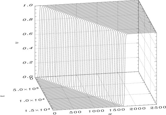
Figure 19: Fuel concentration profile $v(x,t)$ obtained by numerical integration of (29) for $\beta=1$ and $r=0.01$.

Solutions to (29) for different values of $\beta$ and $r=0.01$ are also calculated. The travelling front is found to be stable for all trial parameter values. In figure 20 we plot the speed of the travelling front as function of $\beta$ for $r=0.01$. The numerical results obtained from direct integration of the system of ODEs (5) (solid line) and PDEs (squares) are represented on the same graph. The correspondence between the prediction of both approaches is excellent. The discrepancy was found only in the fourth significant digit.

Figure 20: Speed of the travelling front solution as a function of $\beta$ for $r=0.01$. The solid curve represents the results of integrating the system of ODEs (5), whereas the squares correspond to the results obtained from integrating the governing PDEs (29) integration.

It is interesting to study the behaviour of the solution of the governing PDE (29) for various values of $\beta$ above $\beta_{m}$ in order to investigate if the flame can exist beyond the critical extinction condition. We integrate equations (29) for $r=0.01$ and $\beta=2.5>\beta_{m}$. For all trial initial conditions of the form discussed above, the solution decays to the equilibrium state $u(x,t)=0$ and $v(x,t)=1$ with typical solution profiles shown in figures 21 and 22. The maximum temperature $u(0,t)$ drops rapidly in time to zero and subsequently the reaction ceases and the reaction terms vanish in (29) and the system exhibits almost linear diffusion to the equilibrium state. This is clearly seen in figure 23 which shows the dependence of the squared inverse maximum temperature upon time. The numerical results obtained with the integration of the governing equations (29) (dashed line) are compared with the analytical prediction (solid line), which was found by considering equations (29) without any reaction terms (i.e. we consider only the diffusion effects) with initial conditions as described above. In this case it can be shown that in the limit $t\rightarrow\infty$ the asymptotic behavior of the maximum temperature satisfies $u(0,t)^{-2}=\pi\beta^{2}t/x_{0}^{2}(1-\sigma)^{2}$, which is shown with a solid line on the figure 23. The numerical results are shifted from the asymptotic prediction, especially near the starting point $t=0$. However for larger values of $t$ the maximum temperature follows the diffusion law derived from the linear diffusion equations.

Figure 21: Temperature profile $u(x,t)$ obtained by numerical integration of (29) for $\beta=2.5$ and $r=0.01$.

Figure 22: Fuel concentration profile $v(x,t)$ obtained by numerical integration of (29) for $\beta=2.5$ and $r=0.01$.

Figure 23: Decay of the maximum temperature $u(0,t)$ of (29) solution with time for $r=0.01$ and $\beta=2.5.$ Dashed line represent numerical results and solid line shows the analytical estimate of decay rate.

4 Conclusions and discussions

In this paper we have studied combustion wave propagation in an adiabatic model with two-step chain branching reaction mechanism. The current work extends our previous preliminary investigation of chain branching flames [20]. In contrast to [15] we are not using the activation energy asymptotic approach and consider the model for general values of activation energy. We have also used different non dimensional parameters which enabled a more convenient comparison between the properties of one- and two-step models.

It is demonstrated that the model exhibits travelling combustion front solutions. The properties of these solutions differ form the properties of one-step models. Combustion waves are found to exist in certain regions of the parameter space and are characterized by non zero residual amount of reactant, $\sigma$, left behind the travelling wave. This is not possible in one-step adiabatic flame models as all the fuel is used up in such models. To some extend this characteristic of the two-step adiabatic model is similar to the properties of premixed combustion waves in nonadiabatic one-step models, which can also exist in a certain region of parameter space and exhibit extinction as the boundaries of this region are reached. However the behaviour of the travelling combustion waves near the extinction condition are completely different in these two types of models. In the one step nonadiabatic model the point of extinction corresponds to the turning point of the dependence of flame velocity on parameters (which is a two-valued function), therefore the speed of the wave is always positive. In our two-step model studied here the flame velocity is a single valued function and the velocity drops down to zero as the extinction condition is reached. It is remarkable that at the extinction condition there exist a flame characterized by stationary distribution of temperature, reactant and radicals i.e. a standing combustion wave.

The boundaries of existence for combustion front are determined. We show that for a fixed value of $r$ (dimensionless recombination rate) travelling wave solution branch occupy a certain region in the parameter space which lies outside the region bounded by the curve $\beta_{e}(\sigma)$ which has a maximum $\beta_{m}$ at $\sigma_{m}$ so that $\beta$ remains less than or equal to $\beta_{m}$ and a residual amount of fuel less than $\sigma_{m}$. The maximum values $\beta_{m}$ and $\sigma_{m}$ are achieved at the point of extinction.

The properties of the travelling front solution are studied both analytically using the matched asymptotic analysis and numerically via the integration of the governing PDEs (29) and the ODE formulation of the travelling wave solution (5). The matched asymptotic analysis allowed us to obtain the properties of the travelling front solution near the point of extinction. The asymptotic expression for the speed of the front is obtained as well as the location of the solution branch in the parameter space. In particular, it is shown that for a fixed value of $r$ the speed of the front and $\beta$ are quadratic functions of $\sigma-\sigma_{m}$ near the point of extinction. The results of the asymptotic analysis are then compared with the results obtained by the integration of the governing ODEs for the travelling wave solutions by the relaxation method as described in [4, 18]. It is demonstrated that the results obtained from these two approaches are in excellent agreement. The speed of the front and the location of solution branch in the parameter space are studied in detail for a broad range of parameter values by means of numerical integration of the ODEs. The results of this investigation are then compared with the direct numerical integration of the governing PDEs and are shown to be in an excellent agreement. The stability of the travelling front solution is investigated numerically by employing the Evans function method. It is shown that the classical travelling front solution is stable for all parameter values. These results are also confirmed by direct numerical integration of the governing PDEs. We also compare the results of our paper with the results obtained in [15] in the limit of high activation energy and show that they qualitatively agree.

In this paper we considered the case when the diffusivity of fuel and radicals are equal: $\tau=\tau_{A}=\tau_{B}$. Moreover, for the sake of simplicity it is assumed that these diffusivity are both equal to the heat diffusivity: $\tau=1$. Using these assumptions we found that the classical travelling solution is stable for the whole range of parameters $r$, $\beta$, and $\sigma$ where the solution exists. Similar situation was observed for the one-step nonadiabatic flames. In [18] it was shown that for $\tau=1$ one of the travelling front solution branches was stable for all parameter values where the solutions exist. However, for different values of $\tau<1$ the situation changes due to the presence of the Bogdanov-Takens bifurcation. Therefore, one of the most important issues for further investigation is to understand how the stability of the solutions changes in the chain-branching model for different values of $\tau$.

5 Acknowledgments

The authors are thankful to R.O. Weber for his helpful discussions. VVG would like to thank the University of New South Wales for the grant PSO7264 which enabled him to visit UNSW at ADFA, where the majority of this work was completed and acknowledge the financial support from the Russian Foundation for Basic Research: grants 05-01-00339, 05-02-16518, 06-02-17076 and Russian Academy of Sciences: program ”Problems in Radiophysics”.

References

- [1] Merzhanov, A. G. & Rumanov, E. N., Rev. Mod. Phys. 71, 1173 (1999).
- [2] Makino, A., Prog. Energy Combust. Sci. 27, 1 (2001).
- [3] Zeldovich, Ya. B., Barenblatt, G. I., Librovich, V. B., & Makhviladze, G. M., The mathematical theory of combustion and explosions, Consultants Bureau (New York, 1985).
- [4] Gubernov, V. V., Mercer, G. N., Sidhu, H. S., & Weber, R. O., SIAM J. Appl. Math. 63, 1259 (2003).
- [5] Westbrook, C. K., & Dryer, F., Combust. Sci. Tech. 27, 31 (1981).
- [6] Warnatz, J., Maas, U., & Dibble, R.W.,Combustion: physical and chemical fundamentals, modelling and simulation, experiments, pollutant formation, Springer (Berlin, 1996).
- [7] Pitsch, H., & Bollig, M., FlameMaster, A Computer Code for Homogeneous and One- Dimensional Laminar Flame Calculations, RWTHAachen (Institut fur Technische Mechanik, 1994).
- [8] Sánchez, A. L., Balakrishnan, G., Linan, A., & Williams, F. A., Combust. Flame 105, 569 (1996).
- [9] Sánchez, A. L., Lepinette, A., Bolling, M., Linan, A., & Lazaro, B., Combust. Flame 123, 436 (2000).
- [10] Bechtold, J.K., & Law, C.K., Combust. Flame 97, 317 (1994).
- [11] Seshadri, K., Peters, N., & Williams, F. A., Combust. Flame 96, 407–427 (1994).
- [12] Clavin, P., Fife, P., Nicolaenko, B., SIAM J. Appl. Math. 47, 296–331 (1987).
- [13] Joulin, G., Linan, A., Ludford, G. S. S., Peters, N., Schmidt-Laine, C., SIAM J. Appl. Math. 45, 420–434 (1985).
- [14] Dold, J. W., Weber, R. O., Thatcher, R. W., & Shah, A. A., Combust. Theory Modelling 7, 175-203 (2003).
- [15] Dold, J. W. & Weber, R. O., Reactive-Diffusive stability of planar flames with modified Zeldovich-Liñán kinetics, in Simplicity, Rigor and Relevance in Fluid Mechanics. A volume in honor of Amable Lin a’n, Editors: F.J. Higuera, J. Jime’nez, J.M. Vega, CIMNE, Barcelona 2004.
- [16] Simon, P. L., Kallidasis, S., & Scott, S. K., IMA J. Appl. Math. 68, 537–562 (2003).
- [17] Please, C.P., Liu, F., McElwain, D. L. S., Comb. Theory Mod. 7, 129–143 (2003).
- [18] Gubernov, V. V., Mercer, G. N., Sidhu, H. S., & Weber, R. O., Proc. R. Soc. Lond. A 460, 1259 (2004).
- [19] Weber, R. O., Mercer, G. N., Sidhu, H. S., & Gray, B. F., Proc. R. Soc. Lond. A 453, 1105 (1997).
- [20] Gubernov, V. V., Sidhu, H. S., & Mercer, G. N., J. Math. Chem., 39, 1–14 (2006).
- [21] Evans, J. W., Indiana Univ. Math. J., 22, 577-594 (1972).
- [22] Henry, D., Geometric theory of semilinear parabolic equations, Springer–Verlag ( New York, 1981).
- [23] FlexPDETM http://www.pdesolutions.com