Developing the Theory of Flux Limits from $\gamma$-Ray Cascades

Abstract

Dark matter annihilation and other processes may precipitate a flux of diffuse ultra-high energy $\gamma$-rays. These $\gamma$-rays may be observable in present day experiments which observe diffuse fluxes at the GeV scale. Yet the universe is presently opaque to $\gamma$-rays above 10 TeV. It is generally assumed that cascade radiation is observable at all high energies, however the disparity in energy from production to observation has important consequences for theoretical flux limits. We detail the physics of cascade radiation development and consider the influence of energy and redshift scale on arbitrary flux limits that result from electromagnetic cascade.

I Introduction

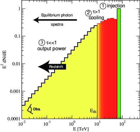
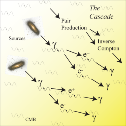
Figure 1: The pair-photon cascade cycles $\gamma$-rays through a series of steps that cool these $\gamma$-rays while conserving energy overall. The total injected power is observable in output spectra. First, diffuse isotropic sources inject $\gamma$-rays above the threshold energy (1). Next these $\gamma$-rays cool through pair production and inverse Compton scattering (2). Finally, the cooled $\gamma$-ray spectrum is observable as a spectrum of inverse Compton photons (3).

The GZK process produces a flux of ultra high-energy $\gamma$-rays. These gamma rays are scattered by the CMB. Furthermore, recent work concerning dark matter annihilation into $\gamma$-rays suggests this is an important pathway for constraining and revealing the nature of dark matter particles Ullio:2002pj . Evidently the universe is replete with non standard model particles. These particles must account for roughly 90% of the matter budget for the universe as a whole. While the galaxy scale distributions of these particles remain in contention, it is known that on large scales dark matter particles are distributed with relative uniformity. Any uniform distribution of particles that annihilate to $\gamma$-rays are subject to substantial observational constraints in both existing and planned experiments. A caveat occurs when these particles are produced above the threshold energy for pair production at cosmological scales. The flux of particles at Earth may be mitigated by cosmogenic propagation. Therefore, before one may constrain particle fluxes based on electromagnetic cascades, one must have a detailed understanding of cascade development, energy scale, production time scale and detector sensitivity.

In addition, the origin of the diffuse extragalactic component of EGRET observations is a deeply held mystery in $\gamma$-ray astrophysics Bergstrom:2001jj ; Taylor:2002zd ; Strong:2004ry . In the galaxy it is predicted that inverse Compton scattering of cosmic-ray electrons on interstellar photons may be the source of diffuse $\gamma$-ray emission Strong:1998pw ; Moskalenko:1998gw . Alternatively, both cosmological and exotic ultra-high energy processes may contribute a portion of the extragalactic $\gamma$-ray spectrum. Fermi shock acceleration may inject ultra-high energy cosmic-ray electrons beyond the TeV scale Gaisser:2006ne . All of these extragalactic high-energy processes are rare and diffuse. If these processes contribute $\gamma$-rays above the pair production threshold, then the determination of the observable spectra resulting from diffuse isotropic cosmological injection is an essential precursor to considering astrophysical models.

II The Cascade

An isotropic injection of ultra-high energy $\gamma$-rays is subject to the pair-photon cascade. The cascade was suggested as early as 1948 Feenberg:1948 , however it was described in detail by Bonometto and Rees in 1971 Bonometto:1971 . This process results when the coupled chain reaction of pair production (1) and inverse Compton scattering (2) is possible.

$$\gamma\gamma\rightarrow e^{+}e^{-}$$ (1)

$$e\gamma\rightarrow e\gamma$$ (2)

Berezinsky illustrates the basic argument in several works Berezinsky:1975 ; Berezinsky:1990 ; Berezinsky:1999az . First, an incoming high energy $\gamma$-ray encounters a thermal background photon and forms an $e^{+}e^{-}$ pair. Pair production is the subject of a useful review by Motz, Olsen, and Koch Motz:1969 . At low energies, with s-wave scattering, the outgoing electron and positron share the incoming total energy:

$$E_{e}=E_{\gamma}/2$$

At high energies, a leading particle carries away most of the incoming energy. This is the forward scattering limit. The threshold for pair production presents an absolute lower bound on the energy where the cascade may occur. This threshold depends on the average energy of isotropic target photons, $\epsilon_{0}$, and the mass of the electron. At present this value is:

$$E_{th}=m_{e}^{2}/{\epsilon_{0}}=10~{}\left({\epsilon_{0}\over{5\times 10^{-3}~{}{\rm eV}}}\right)~{}\,{\rm TeV}$$

At this energy the target distribution is given by the infrared background, while at PeV leading energies the cosmic microwave background may participate. For linear cascades, which develop in low density regions of the universe, the products of cascade development do not participate directly, therefore it is safe to assume that the target distribution is mono-energetic, as in the following brief discussion. Later the thermal photon spectra is presented along with the kinetic solution. Stawarz and Kirk discuss non-linear cascades in a recent work Stawarz:2007hu .

In all of the past discussions of cascade development, one crucial factor is typically under represented. The background distributions of target photons typically evolve rapidly with redshift, $\epsilon=\epsilon_{0}\,{(1+z)}$ Stecker:2005qs . We will see that redshift plays an important role in observability of cascade fluxes.

After pair-production occurs on target photons, the resulting stream of high energy electrons and positrons are susceptible to inverse Compton scattering. Through inverse Compton scattering the energy of these electrons or positrons is transferred into a background photon which results in a new high energy outgoing $\gamma$-ray. The electrons and positrons are left behind and do not participate further. The vast majority of the incoming energy is carried by the outgoing $\gamma$-ray. In the low energy limit, the average energy loss fraction is Gould:1975 .

$$f={\Delta E\over E}\simeq{4\over 3}{{E\epsilon_{0}}\over m_{e}^{2}}$$ (3)

An outgoing electron or positron resulting from $\gamma$-ray injection at threshold will have energy:

$$E_{e}={1\over 2}m_{e}^{2}/\epsilon_{0}$$

Thus, the Cascade will exhibit a transition energy when outgoing $\gamma$-rays no longer have sufficient energy to initiate pair production. This transition energy, called the critical energy, $E_{c}$, is the energy of an outgoing inverse Compton scattered $\gamma$-ray resulting from an electron or positron produced with energy $E_{th}/2$.

$$E_{\gamma,out}=fE_{e}$$

or

$$E_{c}=E_{\gamma,out}={4\over 3}E_{e}^{2}\epsilon_{0}/m_{e}^{2}={1\over 3}E_{\gamma,th}$$

At present, the cascade begins to transition from recycling to emission above 3 TeV. This process is depicted in Fig. 1. The net effect of the cascade is the reprocessing of one incoming high energy $\gamma$-ray into pairs of outgoing $\gamma$-rays, each with roughly half of their parent’s energy. These pairs form others until numerous final particles result. All of these final particles combined share the energy of the incoming $\gamma$-ray.

There are two important energy scales for cascading particles. Below the energy of transition and above. Above $E_{c}$, energy is conserved by the cascade process, therefore we may immediately write the spectrum, $E^{2}dN/dE=const$. Below $E_{c}$, the last generation of $\gamma$-rays are unable to pair produce, therefore they must escape after inverse Compton scattering which has no low energy threshold. These $\gamma$-rays lose energy and conserve number. A deduction of this spectrum is given in App. A.

$${dN\over dE}=\begin{cases}AE^{-2}&E>E_{c}\\ A^{\prime}E^{-3/2}&E<E_{c}\\ \end{cases}$$ (4)

This conventional approximation to the cascade is prevalent in many studies of $\gamma$-ray fluxes. The analysis presented considers the effect of one step of the cascade and allows for reasonable approximations to be made for given models. It is also very simple to consider the effects of two cascade steps. This derivation is given in App. B. Finally, for a multi-stage cascade the following approximation is appropriate:

$${dN\over dE}=\begin{cases}AE^{-2}&E>E_{th}\\ A^{\prime}E^{-3/2}&E_{c}<E<E_{th}\\ A^{\prime\prime}E^{-1}&E<E_{c}\\ \end{cases}$$ (5)

The cascade conserves total energy as it cools the incoming $\gamma$-rays and one exploits this to fix the relation between injection spectra and emission spectra and to determine the normalization constants.

This discussion is essentially complete less one crucial detail. While present observations exist at GeV energies, the present value of $E_{c}$ is about 10 TeV. In order to develop limits on particle fluxes we must consider this issue. The opacity of the universe evolves in redshift. Present experiments will have sensitivity to electromagnetic cascades which develop at $z\approx 1$ and beyond. If cascade radiation is produced only at present, it may only connect with present diffuse observations through extreme downscattering.

All cascade flux limits are deduced from the assumption that the energy density of cascade radiation does not exceed experimental sensitivity as in Fig. 2. For an energy density $\rho$ [GeV/cm³], the following relation is true today:

$$\rho_{cas}<\rho_{obs}$$ (6)

The flux limit on particles injected above $E_{c}$ directly follows from this relation:

$$\left(E^{2}{d\Phi\over dE}\right)_{in}<\,\left(E^{2}{d\Phi\over dE}\right)_{obs}={c\over{4\pi}}\rho_{obs}$$

The most important relevant observation is from EGRET, see Fig. 2. The EGRET experiment on-board the Compton $\gamma$-ray observatory has set an upper bound at 30 GeV of roughly $10^{-6}$ GeV cm^-2 s^-1 sr^-1 Strong:2004ry .

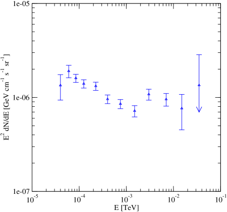
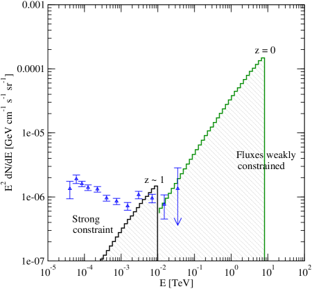
Figure 2: EGRET is sensitive to extragalactic $\gamma$-ray backgrounds below 30 GeV (left) Strong:2004ry . When compared with fluxes of cascading particles it is evident that experimental limits made at present apply only above $z\approx 1$ (right).

Therefore there are two ways to develop cascade limits based on observations at present. Either cascade limits must be deduced from a prior epoch when the universe was opaque to $\gamma$-rays at 30 GeV, i.e. $z\approx 1$, or limits must incorporate the emission spectrum of $\gamma$-rays below $E_{c}$ to decide what part of the present era flux contributes to a particular experiment.

First, it is straight-forward to predict the redshift effects on cascade radiation. Consider, the cascade radiation in a comoving volume ${\cal V}$ defined for an arbitrary but fixed number of cascade particles. Then by (6), $\rho_{cas}{\cal V}<\rho_{obs}{\cal V}$ is also true. However, ${\cal V}$ may be parameterized by a scale factor $a(t)$, and coordinate representation $F({\bf r})$, ${\cal V}=4/3\pi a^{3}F^{3}$. Since $a$ parameterizes all time dependence and similarly $F$ all spatial dependence one may easily conclude that, $\rho_{cas}a^{3}<\rho_{obs}a_{0}^{3}$ is always true. Here $a_{0}$ is used to reference the present day value of the scale factor. This is more customarily written in terms of redshift:

$$\rho_{obs}>\rho_{cas}({a\over a_{0}})^{3}={\rho_{cas}\over(1+z)^{3}}$$

These redshift effects are generally canceled by source evolution with density, i.e. $n=n_{0}(1+z)^{3}$.

Alternatively, cascade radiation may be contributed by downscattering of final stage cascade electrons and positrons. We will treat this spectral development in detail below, yet one can make an initial estimate by taking inverse Compton scattering to have an $E^{-3/2}$ spectrum. By (6), for emission below $E_{c}$ and observation at $E_{obs}$ one has $\rho_{obs}N_{\gamma}>\rho_{cas}N_{\gamma}$ or $\rho_{obs}E_{obs}^{-3/2}>\rho_{cas}E_{c}^{-3/2}$. As in the case of EGRET observations, if $E_{c}/E_{obs}\approx 100$, then the correction factor will be $1/1000$. Even GLAST will only reduce this to $1/100$. Unfortunately, present day cascade radiation will almost certainly not contribute to present day experimental observation through this mechanism. Eq. (6) must be extended with the following relation:

$$\rho_{cas}^{\prime}(E)=\int_{E}^{E_{max}}{dE^{\prime}\int_{0}^{\infty}{dz{{\rho_{cas}(E_{c}(z)=E^{\prime})}\over{(1+z)^{3}}}\left({E_{c}\over E^{\prime}}\right)^{-3/2}}}$$ (7)

From this one may directly consider a few simple cases:

1. Present era high energy injection and observation at $E_{c}$: In this case $\rho_{cas}^{\prime}=\rho_{cas}(E_{c})$.

2. Present day high energy injection and observation somewhat below $E_{c}$. In this case one has a $(E_{c}/E_{obs})^{-3/2}$ penalty:

   $$\rho_{cas}^{\prime}=\rho_{cas}\left({E_{c}\over E_{obs}}\right)^{-3/2}$$

   For the currently practical case of EGRET, contributions to cascade limits by these fluxes are ruled out by a factor of $1/1000$. This could only result in very weak limits on particle fluxes.

3. Observation of a 30 GeV process with significant contributions at $z=1$. This might be considered the ’standard’ or conventional case. Here the best case contribution is:

   $$\rho_{cas}^{\prime}={\rho_{cas,z=1}\over 2^{3}}$$

Consideration of other processes requires a more detailed discussion, however it is already evident that $\gamma$-ray cooling has important consequences for cosmological production processes. Any $\gamma$-rays injected above $E_{th}$ may be observable below this energy. The source of the diffuse flux of $\gamma$-rays below 30 GeV is an open question for astrophysics. However, The energy resulting from cascade $\gamma$-rays is narrowly distributed around $E_{c}$ with little or no contribution as energies approach 30 GeV. These fluxes are suppressed by three orders of magnitude. Important cosmological processes would have to inject enormous amounts of energy above $E_{th}$ to even partially contribute to EGRET diffuse observations today. Therefore it is unlikely that the source of the EGRET diffuse observation is local $\gamma$-ray injection above $E_{th}$.

III Saturated Pair Cascades and Differential Fluxes

Let us now turn to the saturated pair-photon cascade problem to develop a more detailed spectral understanding of cascading particles. For cosmogenic processes one is only concerned with saturated propagation. High energy injection processes are defined to be saturated if through extremes of cosmological scale or density all injected $\gamma$-rays eventually must pair produce Svensson:1987 . In short, the universe is completely opaque to these particles. Obviously, this calculation is not sensitive to conditions in which the universe is not completely opaque. The cascade does not conserve particle number so repeated solution of scattering relations is required to determine a final emission spectrum.

To solve saturated propagation it is customary to employ the method proposed by Guilbert Guilbert:1981 . An integral kinetic equation gives the spectra resulting from sources. The cross sections of $\gamma$-ray scattering are well known. It is possible to directly calculate the probability of a $\gamma$-ray scattering from a given energy to any other energy. Repeated convolution of the scattering probability with the incident number distribution finally determines the resulting spectrum.

Svensson and Zdziarski Zdziarski:1985 ; Svensson:1987 ; Zdziarski:1988 ; Zdziarski:1989 ; Zdziarski:1989a ; Zdziarski:1989b ; Svensson:1990 ; Nath:1990 considered the cascade problem extensively using a similar analytical approach. The steady-state solution to a kinetic equation of propagation allows an analytical determination of final spectra based solely on rate and injection models. If electron escape is neglected, then the steady state electron distribution is completely described by electron production and energy loss.

This solution applicable to diffuse cosmological processes makes the following assumptions.

1. A narrow isotropic distribution of $\gamma$-rays is injected above $E_{th}$. This may similarly be solved for power laws and other distributions.

2. The interaction scale for photons and electrons is short (10 Mpc) in comparison with propagation scales (Gpc). Therefore, cosmogenic injection processes are saturated above the pair-production threshold, $E_{th}$.

3. The universe is pervaded by an isotropic distribution of soft background photons at a recent epoch, $z<0.03$. This solution may be extended to higher redshifts without difficulty.

4. The energy loss time-scale for electrons is negligible in comparison with any possible escape time-scale.

5. Any homogeneous magnetic fields present on cosmological scales have a negligible effect on energy loss.

Based on these assumptions, a self-consistent solution to the saturated pair cascade problem in the ultra-high energy low redshift regime follows. The observable $\gamma$-ray spectrum below $E_{c}$ is then deduced. It turns out that the isotropic cosmological background acts as a photon calorimeter, while the conformation of any injected spectra are lost, total energy of injection is preserved and observable in experiments with sensitivity near $E_{c}$.

IV Interactions of Cosmological $\gamma$-Rays and Electrons

Cosmological $\gamma$-rays and electrons may be susceptible to energy loss through inverse Compton scattering, pair production, photon-photon scattering, Compton scattering, synchrotron radiation and redshift. One may briefly summarize the effects of these processes to deduce the important propagation processes. In the conventional notation for dimensionless energy, one refers to photon energy with $\omega=E_{\gamma}/m_{e}$ and electron Lorentz factor $\gamma=E_{e}/m_{e}$.

Incident Particle	Process	Target Density [cm-3]	Cross Section [$\sigma_{T}$]	$\lambda$ [Mpc]
Gamma Rays
	$\gamma\gamma\rightarrow e^{+}e^{-}$ on CIB (TeV)	0.5	$3/16$	$10$
	$\gamma\gamma\rightarrow e^{+}e^{-}$ on CMB (PeV)	$410.5$	$3/16$	$10^{-2}$
	$\gamma e\rightarrow\gamma e$	$10^{-7}$	$10^{-3}$	$10^{10}$
Electrons and Positrons
	$e\gamma\rightarrow e\gamma$ on CIB (TeV)	0.5	1	$1$
	$e\gamma\rightarrow e\gamma$ on CMB (PeV)	410.5	1	$10^{-2}$

Table 1: Inverse Compton scattering and pair production are important cosmological loss processes for electrons and $\gamma$-rays.

IV.0.1 Pair Production from $\gamma$-Rays

To estimate the scattering length for $\gamma$-rays I assume cosmological $\gamma$-rays will pair-produce on an isotropic infrared background if $\epsilon_{\gamma}\approx 10$ TeV. The center of mass energy squared for TeV gamma-rays against infrared background photons is $s\approx 4\epsilon_{\gamma 1}\epsilon_{\gamma 2}\approx 10^{-13}$ TeV², the dimensionless center of mass energy is $\sqrt{\omega_{1}\omega_{2}}\approx 1$. The cross section is found at the peak of the pair production rate $\sigma\approx{3\over 16}\sigma_{T}$. The Thomson cross section, $\sigma_{T}$, is related to the classical electron radius by $8\pi r_{e}^{2}/3$. The mean interaction length for cosmogenic pair production is about 10 Mpc. This mean free path is minimized for injected gamma-rays at PeV energies. In this case, the interaction length drops to about 10 kpc because of the increased density of microwave background targets.

$$\lambda_{\gamma\gamma\rightarrow e^{+}e^{-}}={1\over n\sigma}\approx 10\,{\rm Mpc}$$

In comparison with the Hubble scale, pair production is a primary energy loss mechanism for cosmological $\gamma$-rays with energy above $E_{th}$.

IV.0.2 Compton Scattering of Gamma-Rays

Compton scattering of a cosmological $\gamma$-ray on a primordial electron is primarily important at epochs where primordial electron density is significant. A TeV $\gamma$-ray and background electron system has center of mass energy squared, $s\approx 4\epsilon_{\gamma}m_{e}\approx 10^{-6}$ TeV². In dimensionless form, $\sqrt{\omega\gamma}\approx 3000$, the cross section for TeV $\gamma$-rays is $\sigma\approx 10^{-3}\sigma_{T}$ – $10^{-5}\sigma_{T}$. The density of primordial electrons is roughly equivalent to the density of baryons, $n_{e}\approx n_{b}\approx 10^{-7}$ cm^-3. The mean interaction length of Compton scattering is only significant at high redshifts.

$$\lambda_{\gamma e\rightarrow\gamma e}={1\over n\sigma}\approx 10^{10}\,{\rm Mpc}$$

The mean free path for Compton scattering is so large that I take these losses to be negligible.

IV.0.3 Photon-Photon Scattering of Gamma-Rays

Photon-photon scattering, $\gamma\gamma\rightarrow\gamma\gamma$, is an important cosmological consideration at high redshift and low energy scales when the universe was radiation dominated. Svensson and Zdziarski treat this process in detail in Svensson:1990 . I neglect this scattering process here under the assumption of ultra-high energy propagation in a matter dominated epoch.

IV.0.4 Inverse Compton Scattering of Electrons and Positrons

Cosmological electrons of TeV energies may scatter on isotropic primordial photons. The center of mass energy squared is $s\approx 4E_{e}\epsilon_{\gamma}$. The electron energy, $E_{e}$, is about 1 TeV. The energy of infrared photons averages about $10^{-2}$ eV, so the dimensionless center of mass energy is $\sqrt{\omega\gamma}\approx 0.5$. This is well within the Thomson regime so the cross section is the Thomson cross section. The density of soft infrared target photons is $0.5$ cm^-3. The interaction length of TeV electrons is about one Mpc. This is a rough estimate made for illustrative purposes, the integration below uses exact distributions. This interaction length is minimized when the CMB can participate. At PeV energies the interaction length of an electron drops to about 1 kpc.

$$\lambda_{e\gamma\rightarrow e\gamma}={1\over n\sigma_{T}}\approx 1\,{\rm Mpc}$$

As a result inverse Compton scattering is a primary energy loss mechanism for cosmological electrons above one TeV.

IV.0.5 Synchrotron Radiation from Electrons and Positrons

Cosmological electrons in a magnetic field, ${\bf B}$, emit $\gamma$-rays as they accelerate through a helical trajectory. The energy loss through this mechanism is proportional to magnetic energy density or ${\bf B}^{2}$.

$${dE\over dt}\approx{4\over 3}\sigma_{T}c\beta^{2}\gamma^{2}{{\bf B}^{2}\over 8\pi}$$

The cosmological magnetic field density has been constrained at less than $10^{-12}$ Gauss. Since synchrotron loss depends on ${\bf B}^{2}$, I assume that cosmological magnetic fields may be neglected in this calculation. See Blumenthal:1970 for a detailed treatment of this loss process.

IV.0.6 Redshift

The energy loss scale due to redshift is of roughly the same order as the Hubble length scale.

$$\lambda_{z}\approx{c\over H_{0}}\approx 4\,{\rm Gpc}$$

The extension of this solution to include detailed accounting of redshift is straightforward but not required since the principal loss processes are far faster than this mechanism.

V Production in Astrophysical Processes

For particles susceptible to these interactions a particular isotropic injection has flux defined by

$$\Phi={c\over 4\pi}\int_{E_{min}}^{E_{max}}{dE\,{dN\over dE}}$$ (8)

The differential number density is taken as $dN/dE$ [GeV^-1 cm^-3]. Where $dN/dE\ dE$ represents the number of particles in an interval $(E,E+dE)$ per volume. If $N_{0}$ represents the density today, the density evolves with redshift, $z$.

$$N=N_{0}(1+z)^{3}$$

The flux of particles resulting from a particular astrophysical process is determined by the production rate. Rate is given by (9), expressed in terms of the incident particle distribution $n$, and reaction cross section, $\sigma$.

$$\Gamma(E^{\prime},E)=c\int_{\epsilon_{min}}^{\epsilon_{max}}{d\epsilon\ n(\epsilon)\int_{E_{min}}^{E_{max}}{dE^{\prime}\ {d\sigma\over dE}(E^{\prime},E)}}$$ (9)

The term ${d\sigma\over dE}(E^{\prime},E)$ represents the differential cross section for scattering from a particle of energy $E^{\prime}$ to energy $E$. Also this integral can be normalized over target particle distributions and arbitrary directions. This paper adopts the notation $\mu=\cos{\theta}$ for the scattering angle and uses $\beta$ to refer to velocity. The following equation represents the production from scattering of an isotropic incident distribution on a target distribution across a spectrum of energies.

$$\dot{N}=c\int_{\epsilon_{min}}^{\epsilon_{max}}{d\epsilon\ {n_{T}(\epsilon)}\int_{-1}^{1}{d\mu\ {{1-\beta\mu}\over 2}\int_{E_{Imin}}^{E_{Imax}}{dE_{I}\ n_{I}(E_{I})\int_{E_{min}}^{E_{max}}{dE^{\prime}\ {d\sigma\over dE}(E^{\prime},E)}}}}$$ (10)

In this equation $n_{T}$ represents the distribution of targets and $n_{I}$ represents the distribution of incident particles. I use $\dot{N}$ to represent the first derivative in time, $dN/dt$, hereafter.

VI The Kinetic Equation

The kinetic equation gives the observable spectrum, $N(E)$, of particles after scattering for a given injection spectrum $N_{0}(E)$. The transport of high energy $\gamma$-rays through the cosmological medium involves catastrophic energy loss through pair production. The resulting stream of electrons boosts photons from the primordial background through inverse Compton scattering.

The contributions to $\gamma$-ray energy loss are either continuous or discrete. The continuous radiative transfer of a propagating particle is described as a differential equation over spatial propagation Rybicki:1979 .

$${dN\over dx}(E)=-\alpha N(E)+j$$ (11)

Where $\alpha$ is the coefficient of assumed continuous energy loss and $j$ is the particle injection term. Solutions to (11) reveal the effects of continuous energy loss on an initial spectrum, but do not describe catastrophic loss processes. To consider both types of loss processes one employs a steady-state differential equation.

The observable spectrum of $\gamma$-rays can be deduced by considering the repeated effects of energy loss in multiple scatterings. Since escape is neglected, differential changes in particle flux must be stable.

The electron steady-state is described by loss due to inverse Compton scattering, production of $e^{+}e^{-}$ pairs, and injection Svensson:1987 .

$$\dot{N}_{e}=-\dot{N}_{e,C}(E)+\dot{N}_{e,P}(E)+\dot{N}_{e,in}(E)$$ (12)

Likewise $\gamma$-rays appear after inverse Compton scattering or injection, and disappear in pair production. I will use $n$ (lower case) to label a spectrum of photons and $N$ to label a spectrum of electrons.

$$\dot{n}_{\gamma}=\dot{n}_{\gamma,C}(E)-\dot{n}_{\gamma,P}(E)-c{dn_{\gamma}\over dx}(E)+\dot{n}_{\gamma,in}(E)$$ (13)

In (12) and (13) the subscripts “C” and “P” are used to indicate the time derivative due to inverse Compton scattering (2) and pair production (1) respectively. The radiative transfer is given by $dn/dx$ and (11). The radiative transfer term may be used to model losses from $\gamma\gamma$ absorption in dense environments. The terms with “in” subscripts represent continuous isotropic particle injection. Both equations are independent of charge, therefore electron and positron losses are identical. In order to consider the effects of both electron and positron production one simply doubles the electron production rate. For the remainder of the article I will refer to electrons only, of course in reality half of the denumerable electron population would be physical positrons. This is irrelevant since I only consider the resulting flux of $\gamma$-rays.

For many physical models involving the injection of $\gamma$-rays there are no electron sources, in this numerical integration $\dot{N}_{e,in}=0$, this choice is arbitrary and made for numerical convenience, it would be equivalent to inject first generation electrons or positrons rather than $\gamma$-rays.

Since (12) and (13) are coupled by pair production and inverse Compton scattering, one may adopt the point of view of either electrons or $\gamma$-rays, I choose electrons in consideration of previous work in this field.

Now by considering the known cross sections for inverse Compton scattering and pair production one may write a differential equation describing electron production in terms of energy. Inverse Compton scattering on an isotropic distribution of background photons is given by (14).

$$\dot{N}_{e,C}(E)=c\int_{\epsilon_{min}}^{\epsilon_{max}}{d\epsilon\ {n_{T}(\epsilon)}\int_{-1}^{1}{d\mu\ {{1-\beta\mu}\over 2}\int_{E_{min}}^{E_{max}}{dE^{\prime}\ N_{e}(E^{\prime}){d\sigma_{C}\over dE}(E^{\prime},E)}}}$$ (14)

If the background photons are thermal, the density is integrated from the Planck distribution. The present day temperature is $T_{0}=T_{CMB}=2.725$ K and $k_{b}$ is the Boltzmann constant. In general, $T$ is proportional to $T_{0}(1+z)$. The energy evolves with redshift according to the relation $\epsilon={\epsilon_{0}(1+z)}$.

$$n_{T}(\epsilon)\,d\epsilon={1\over\pi^{2}({\hbar c})^{3}}{\epsilon^{2}\over{\exp{({\epsilon\over k_{b}T})}-1}}d\epsilon$$

The primarily relevant background for $\gamma$-rays at 10 TeV is the infrared background (CIB). I assume this background is adequately described by a power-law and a black body at $T_{CIB}=2725K$. These assumptions are consistent with recently published detailed models of photon backgrounds Dwek:2004pp ; Stecker:2005qs . I arbitrarily normalize to achieve agreement with accepted observations, see citations above for detailed discussions of these backgrounds.

The Compton energy loss rate of electrons is equal in magnitude to the energy production of Compton $\gamma$-rays. For a photon of energy $\omega m_{e}c^{2}$, and an electron of energy $\gamma m_{e}c^{2}$, the exact angle averaged scattering rate for electron disappearance is given by the Klein-Nishina form Coppi:1990 .

$$\dot{N}_{e,C}(\omega,\gamma)=c\int_{0}^{\infty}{d\epsilon\ n_{T}(\epsilon)\int_{2\gamma(1-\beta)\omega}^{2\gamma(1+\beta)\omega}{d\kappa\ N_{e}(\kappa){d\sigma_{KN}\over d\kappa}}}$$ (15)

$${d\sigma_{KN}\over d\kappa}(\kappa)={{3\sigma_{T}}\over 32\gamma^{2}\beta\omega^{2}}\left[\left(1-{4\over\kappa}-{8\over\kappa^{2}}\right)\ln{(1+\kappa)}+{1\over 2}+{8\over\kappa}-{1\over{2(1+\kappa)^{2}}}\right]$$

It is usual to employ a change of variables, $\kappa=2\gamma(1-\beta\mu)\omega$, in this equation. In the low energy (“Thomson”) limit this rate approaches $c\sigma_{T}$, the speed of light multiplied by the Thomson cross section. The Compton rate is depicted in Fig. 3.

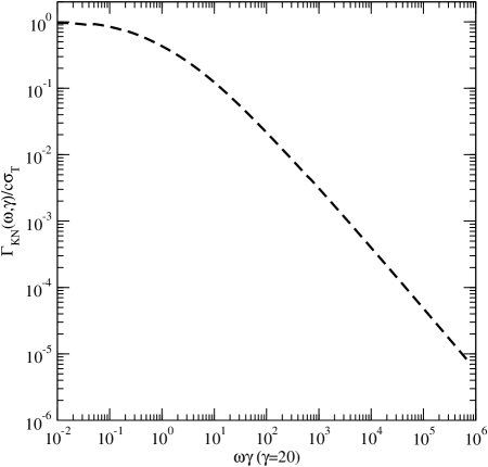
Figure 3: The scattering rate of $\gamma$-rays due to the inverse Compton process (2). Electron energy is fixed at $20m_{e}c^{2}$. This figure corresponds to Coppi and Blandford Fig. 1 Coppi:1990 : given here for comparison. The Compton rate is unusual in that it decreases as energy increases. The maximum rate in the “Thomson” regime occurs at $c\sigma_{T}$. The rate is divided by $c\sigma_{T}$ to reflect the absolute shape of the interaction in dimensionless form.

Equation (15) can be analytically integrated and this is a common step for several authors including Zdziarski, however the resulting rate is a complicated function involving dilogarithms. There may be no computational or intellectual benefit from performing this integration, I omit it. In either case one is required to numerically integrate over the rates to deduce a final spectrum. This approach is also suggested by Coppi and Blandford Coppi:1990 .

To clarify the meaning of (15) I introduce a shorthand, $C(E)=-\int_{E_{min}}^{E}{dE^{\prime}d\sigma/dE}$, for the portion of the integral over (14) from $E_{min}$ up to the energy of consideration $E$. It is evident from Fig. 3 that the derivative of the cross section is negative.

$$\dot{N}_{e,C}(E)=c \int_{\epsilon_{min}}^{\epsilon_{max}}{d\epsilon\ {n_{T}(\epsilon)}\int_{-1}^{1}{d\mu\ {{1-\beta\mu}\over 2}\ }}N_{e}(E)$$

$$\times\left(C(E)-\int_{E}^{E_{max}}{dE^{\prime}\ {d\sigma_{C}\over dE}(E^{\prime},E)}\right)$$ (16)

In (VI) the first term represents electron energy loss due to boosted primordial photons, it is positive (loss) because these inverse Compton electrons are scattered to lower energies. The second term represents the appearance of inverse Compton scattered electrons from higher energies. The sign is consistent with (12) which defines this equation as a loss rate.

The pair production or electron appearance rate is given by

$$\dot{N}_{e,P}(E)=c\int_{\epsilon_{min}}^{\epsilon_{max}}{d\epsilon\ {n_{T}(\epsilon)}\int_{-1}^{1}{d\mu\ {{1-\mu}\over 2}\ \int_{E_{min}}^{E_{max}}{dE_{\gamma}\ n_{\gamma}(E_{\gamma})\ {d\sigma_{P}\over dE}(E_{\gamma},E)}}}.$$ (17)

The term ${d\sigma_{P}\over dE}(E_{\gamma},E)$ represents the differential cross section of a photon of energy $E_{\gamma}$ to produce an electron of energy $E$. Eq. (13) reveals that there are two sources of $\gamma$-rays that may take part in pair production, either freshly injected $\gamma$-rays from isotropic sources or $\gamma$-rays boosted through inverse Compton scattering.

$$n_{\gamma}(E)=n_{\gamma,in}(E)+n_{\gamma,C}(E)$$

These two relations are combined in (VI).

$$\dot{N}_{e}(E) =\int_{\epsilon_{min}}^{\epsilon_{max}}{d\epsilon\ {n_{T}(\epsilon)}\int_{-1}^{1}{d\mu\ {{1-\mu}\over 2}\ \int_{E_{P,min}}^{E_{P,max}}{dE_{\gamma}\ {d\sigma_{P}\over dE}(E_{\gamma},E)}}}$$

$$\times \left(\dot{n}_{\gamma,in}(E_{\gamma})+c\int_{E_{C,min}}^{E_{C,max}}{dE^{\prime}\ N_{e}(E^{\prime}){d\sigma_{C}\over dE}(E,E^{\prime}-E_{\gamma})}\right)$$ (18)

The exact photon-photon pair production rate is given by Coppi:1990

$$\dot{N}_{e,P}=c\int_{0}^{\infty}{d\epsilon\ n_{T}(\epsilon)\int_{-1}^{\mu_{max}}{d\mu\ {{1-\mu}\over 2}\ \int_{E_{min}}^{E_{max}}{dE_{\gamma}\ n_{\gamma}(E_{\gamma}){d\sigma_{\gamma\gamma}\over dE}}}}$$ (19)

$${d\sigma_{\gamma\gamma}\over dE}={3c\sigma_{T}(1-\beta^{\prime 2})\over 16}\left[(3-\beta^{\prime 4})\ln{\left({{1+\beta^{\prime}}\over{1-\beta^{\prime}}}\right)}-2\beta^{\prime}(2-\beta^{\prime 2})\right].$$

Following standard notation, dimensionless parameters for photon energy are $\omega_{1}=\epsilon/{m_{e}c^{2}}$ and $\omega_{2}=E_{\gamma}/{m_{e}c^{2}}$, so $\mu_{max}={\rm max}(-1,1-2/{\omega_{1}\omega_{2}})$. The electron velocity is $\beta^{\prime}=[1-2/{\omega_{1}\omega_{2}}(1-\mu)]^{1/2}$. The pair production rate is depicted in Fig. 4.

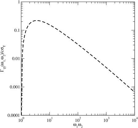
Figure 4: The scattering rate of a photon of energy $\omega_{1}m_{e}c^{2}$ against a photon of energy $\omega_{2}m_{e}c^{2}$ to form electron-positron pairs (1). This figure corresponds to Coppi and Blandford Fig. 5 Coppi:1990 : given here for comparison. The pair production rate peaks at about $3\sigma_{T}/16$ and then falls off as energies increase. The rate is divided by $c\sigma_{T}$ to reflect the absolute shape of the interaction in dimensionless form.

For extragalactic cosmic media it is assumed that the inverse Compton scattering and pair production mechanisms entirely describe the cascade energy loss and no additional energy losses are present, $dN/dx=0$. Combining (12), (VI) and (VI) reveals a steady-state integral-differential equation of electron transport.

$$\dot{N}_{e}= -c\int_{\epsilon_{min}}^{\epsilon_{max}}{d\epsilon\ {n_{T}(\epsilon)}\int_{-1}^{1}{d\mu\ {{1-\beta\mu}\over 2}\ N_{e}(E)\left(C(E)-\int_{E}^{E_{max}}{dE^{\prime}\ {d\sigma_{C}\over dE}(E^{\prime},E)}\right)}}$$

$$+\int_{\epsilon_{min}}^{\epsilon_{max}}{d\epsilon\ {n_{T}(\epsilon)}\int_{-1}^{1}{d\mu\ {{1-\mu}\over 2}\ \int_{E_{P,min}}^{E_{P,max}}{dE_{\gamma}\ {d\sigma_{P}\over dE}(E_{\gamma},E)}}}$$

$$\times\left(\dot{n}_{\gamma,in}(E)+c\int_{E_{C,min}}^{E_{C,max}}{dE^{\prime}\ N_{e}(E^{\prime}){d\sigma_{C}\over dE}(E^{\prime},E^{\prime}-E_{\gamma})}\right)$$ (20)

Eq. (VI) is comparable to Zdziarski Equation 1 Zdziarski:1988 , with solutions that show the time evolution of the electron spectrum versus energy. It is possible to eliminate time dependence by considering the continuous energy loss $dE_{C}/dt$ Svensson:1987 .

$$\dot{N}(E)={d\over dE}[{dE_{C}\over dt}N(E)]$$

Here, Zdziarski gives the continuous energy loss in terms of a small parameter $\delta$, I take $\delta$ to be $10^{-4}$ Zdziarski:1988 :

$${dE_{C}\over dt}(E)=\int_{E/(1+\delta)}^{E}{dE^{\prime}\ (E^{\prime}-E)\dot{N}_{e,C}}$$

This alteration gives an equation comparable to Zdziarski Eq. (2) Zdziarski:1988 :

$${d\over dE}[{dE_{C}\over dt}N_{e}]= -c\int_{\epsilon_{min}}^{\epsilon_{max}}{d\epsilon\ {n_{T}(\epsilon)}\int_{-1}^{1}{d\mu\ {{1-\beta\mu}\over 2}\ N_{e}(E)\left(C(E)-\int_{E}^{E_{max}}{dE^{\prime}\ {d\sigma_{C}\over dE}(E^{\prime},E)}\right)}}$$

$$+\int_{\epsilon_{min}}^{\epsilon_{max}}{d\epsilon\ {n_{T}(\epsilon)}\int_{-1}^{1}{d\mu\ {{1-\mu}\over 2}\ \int_{E_{P,min}}^{E_{P,max}}{dE_{\gamma}\ {d\sigma_{P}\over dE}(E_{\gamma},E)}}}$$

$$\times\left(\dot{n}_{\gamma,in}(E)+c\int_{E_{C,min}}^{E_{C,max}}{dE^{\prime}\ N_{e}(E^{\prime}){d\sigma_{C}\over dE}(E^{\prime},E^{\prime}-E_{\gamma})}\right)$$ (21)

This equation for electron transport is a restatement of the condition of steady state equilibrium.

$${d\over dE}[N(E){dE_{C}\over dt}]=N(E)$$

In (VI) $N_{e}$ is present on both sides. Also the dependence on $N_{e}$ is incorporated in several integral terms. The most effective strategy for solving (VI) is to apply the Runge-Kutta technique.

VII Numerical Techniques

The Runge-Kutta technique is a method for iteratively solving a differential equation which has the following form:

$$y_{n+1}=y_{n}+hf(x_{n},y_{n})$$

$$f(x_{n},y_{n})={dy_{n}\over dx_{n}}$$

The solution is advanced through small steps $h$, with $x_{n+1}=x_{n}+h$, and the result is accumulated. An adaptive step size is incorporated to reduce computation time while holding relative errors fixed. The C++ code utilizes 4^th order Runge-Kutta method with 5^th order error checking. It is prudent to recall that higher-order is not synonymous with either smaller error or improved numerical stability. However this technique converges rapidly for (VI). The details of the Runge-Kutta calculation are described in many texts including Numerical Recipes NR:2002 .

I hold absolute errors to $1.0\times 10^{-4}$ at machine precision and relative errors to $0.0$. The equation for electron transport gives solutions for the expected number of particles in a logarithmic energy bin. The initial electron spectrum is null and the initial $\gamma$-ray spectrum is set to unit height in a logarithmic energy bin corresponding to the injection energy. The energy range is divided into an arbitrary number of intervals of constant logarithmic width and (VI) is repeatedly solved starting at higher energies and moving to lower.

The highest energy bin must be solved first since pair production occurs in the highest bins first, and then subsequent electrons downscatter to lower energies over repeated iteration of the cascade process. In other words the electrons first appear in the higher energy bins and move down in energy.

The result of this iteration is an electron spectrum corresponding to the specified photon injection. One final generation of inverse Compton scattering reveals the outgoing $\gamma$-ray production. The output production is integrated from the inverse Compton scattering rate to give the final result Zdziarski:1988 .

$$\dot{n}_{\gamma}(E_{\gamma})=\int_{E_{\gamma}}^{E_{max}}{dE^{\prime}\,N_{e}(E^{\prime})\Gamma_{KN}(E^{\prime},E^{\prime}-E_{\gamma})}$$ (22)

The $\gamma$-ray production is then integrated over the time variable $t$ until the output is fully saturated, i.e., until the observable energy is equal to the injection energy. The solution of (VI) is depicted in Fig. 5. Finally, flux may be determined from (8).

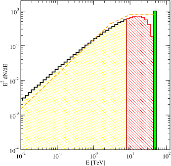
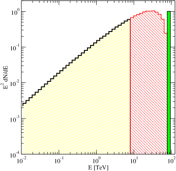
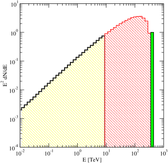
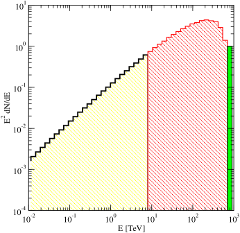
Figure 5: A plot of (22) with solutions of (VI) as input. The 50 TeV (top left), 100 TeV (top right), 500 TeV (bottom left) and 1000 TeV (bottom right) $\gamma$-rays are injected (shown in green) above $E_{th}$. The spectrum resulting from the cascade has two components. The observable portion below $E_{th}$ in black and the continuously propagating portion above $E_{th}$ is depicted in red. Just below the threshold energy of 10 TeV, the height of the resulting spectrum is about $1/2$ the height of the injection. Eq. (5) is superimposed on the 50 TeV injection for comparison.

Applying numerical solution to (VI) shows that during the cascade height (or equivalently energy) is preserved per logarithmic energy interval on an $E^{2}dN/dE$ plot as $\gamma$-rays cool. Fig. 5 shows that the cascade process recycles most of the injected energy until it finally turns off near $E_{c}$, then the resulting spectrum is simply the portion due to inverse Compton scattering. Fig. 5 uses a logarithmic scale where each range represents a fixed interval of constant energy. Energy can be read as the height of the figure. There are a total of 50 constant logarithmic intervals, however this number is chosen arbitrarily to minimize processing time while accurately representing the shape of the output spectrum.

VIII Results for Cascading Particles

As high energy $\gamma$-rays are injected above $E_{th}$, they immediately form pairs and begin cycling through the cascade process, finally just above $E_{c}$ and after many generations, cascading electrons and photons have nearly the same energy as the first generation did. Suddenly, the cascade turns off and most of the energy is preserved in the range $E_{c}$ to $E_{th}$.

Therefore, the cascade acts as a photon calorimeter. About 85% of the energy injected above $E_{th}$ is ultimately observable in the energy decade ($E_{th}/10$, $E_{th}$) near $E_{c}$. However, the cascade does not preserve the conformation of the injected spectrum. While a narrow bin may be injected, the observable spectrum is fixed by the shape of the inverse Compton scattering rate and is not accurately reflected as a simple energy translation of the input bin.

At the factor of two level, one may consider a rule of thumb.

$$E^{2}{dn\over dE}(E_{c})\approx E^{2}{dn\over dE}(E_{in})$$ (23)

This is a naive heuristic which hides the relevant physics, however the conclusion that the majority of the injected power scatters into the energy range at $E_{c}$ is valid. Essentially this relation demonstrates that the cascade conserves energy.

Importantly the energy due to ultra-high energy $\gamma$-ray injection processes is not lost in the sinuous cascade. The total output power is equal to the total input power (conservation of energy) and the rapid ascent of the inverse Compton scattered photon spectrum ensures that most of the observable energy will appear at $E_{c}$. These results clearly rule out a “bin-shifting” approach to $\gamma$-ray energy conservation, however they do provide a number of useful estimates of expected spectral outcomes.

Finally, the cascade takes place extremely rapidly on cosmological scales. Direct computation of redshift effects on cascade spectra is not needed since from the standpoint of cascading particles the universe is essentially flat and static. One may however easily extend the spectrum to produce real cosmological flux limits using (7).

IX Summary

In conclustion, $\gamma$-ray energy injected by ultra high-energy isotropic cosmological processes is observable as a spectrum of cooled $\gamma$-rays. These processes differ from point sources in that point sources suffer attenuation on the cosmological medium.

The consequences of this work may be summarized as follows:

1. Diffuse isotropic injection processes above 10 TeV are constrained by experiments which observe $\gamma$-rays below 10 TeV.

2. The total input power spectrum is reprocessed leading to a $\gamma$-ray pile up at $E_{c}$. This output spectrum gives total integrated limits on injection energy.

3. Observations of present day fluxes suffer important restrictions from both energy and redshift scales. Cosmological processes that contribute to the EGRET diffuse flux observations must be significant at $z\approx 1$. The significance of any observation of present day cascade radiation processes is highly suppressed by a factor of 1000.

There are energy loss processes which I have not considered in these calculations. First the synchrotron losses may have unit order corrections on these calculations where large magnetic fields are present. Next ionization energy losses in dense galactic regions may play a key role in $\gamma$-ray attenuation. Finally, bremsstrahlung losses may give a measurable correction to galactic fluxes.

For all of these loss processes, the rate of loss could easily be measured by considering the emission of well understood sources. In particular, through the synchrotron mechanism this may give a testable method of determination of the intergalactic magnetic fields.

Throughout this discussion I have taken it for granted that the photon injection was continuous and isotropic on the cosmological scale. Individual point sources represent a dramatically different type of propagation problem than what is covered in this work.

X Acknowledgment

I acknowledge my advisor John Beacom for collaboration and helpful suggestions. I thank Hasan Yüksel, Mandeep Gill, Frederick Kuehn, Gregory Mack and Eduardo Rozo for interesting discussions and editorial comments. JAC was supported by DOE Grant No. DE-FG02-91ER40690; I also thank CCAPP and OSU for support.

Appendix A The Spectrum of $\gamma$-rays Scattered at $E_{c}$

Berezinksy derives the spectrum of $\gamma$-rays at $E_{c}$ in his textbook Berezinsky:1990 . In the high energy limit electrons conserve energy, $Eq_{e}(E)=const$, above $E_{c}$. The production of inverse Compton $\gamma$-rays is the number in a logarithmic interval $q_{e}(E_{c})\,dE$ over the width of a logarithmic interval $dE_{e}/E_{\gamma}$, i.e., $dlnE$. The spectrum is:

$$n_{\gamma}=q_{e}(E_{c}){dE_{e}\over E_{\gamma}} \star$$ ()

But as we have said, energy is conserved, therefore at $E_{c}$, $q_{e}=q_{0}$. The energy carried by an outgoing $\gamma$-ray is the fraction liberated from the electron or positron, $E_{\gamma}=fE_{e}$, by Eq. (3):

$$E_{\gamma}={4\over 3}{{E_{e}^{2}\epsilon}\over m_{e}^{2}}$$

Taking the derivative and isolating $dE_{e}$ we have:

$$dE_{e}={1\over 2}{3\over 4}{m_{e}^{2}\over\epsilon}{dE_{\gamma}\over E_{e}}$$

And solving for $E_{e}$:

$$E_{e}=m_{e}\sqrt{{3\over 4}{E_{\gamma}\over\epsilon}}$$

Finally we can combine these relations in ($\star$ ‣ A):

$$n_{\gamma}={1\over 2}q_{0}m_{e}\sqrt{3\over 4\epsilon}\,{dE_{\gamma}\over E_{\gamma}^{3/2}}$$

As expected, at $E_{c}$ the spectrum of $\gamma$-rays is falling as $E^{-3/2}$.

Appendix B The Spectrum of $\gamma$-rays Scattered at Higher Energies

Above, we present the conventional discussion of $\gamma$-ray spectra resulting from a single cascade step. It is trivial to extend this discussion to include an additional step. If the injected particle energy is taken as $4E_{th}$ rather than $E_{th}$ an additional scattering step results. Here the low energy approximation to energy loss fraction does not apply. In this “middle” energy range the outgoing electron and positron share total energy so the loss fraction is now:

$$f\approx{1\over 2}$$

Then the following expression trivially follows from ($\star$ ‣ A):

$$n_{\gamma}=2q_{0}{dE_{\gamma}\over E_{\gamma}}+n_{\gamma,2}$$

In this relation $n_{\gamma,2}$ will be the flux produced by the subsequent outgoing $\gamma$-ray produced at $E_{th}$. Yet we have already deduced this spectrum in App. A. Therefore,

$$n_{\gamma}=2q_{0}{dE_{\gamma}\over E_{\gamma}}+{1\over 2}q_{0}m_{e}\sqrt{3\over 4\epsilon}\,{dE_{\gamma}\over E_{\gamma}^{3/2}}$$

The $E^{-1}$ spectrum will dominate for $E>1$.

References

- (1) P. Ullio, L. Bergstrom, J. Edsjo and C. G. Lacey, “Cosmological dark matter annihilations into gamma-rays: A closer look,” Phys. Rev. D 66, 123502 (2002) [arXiv:astro-ph/0207125].
- (2) L. Bergstrom, J. Edsjo and P. Ullio, “Spectral gamma-ray signatures of cosmological dark matter annihilations,” Phys. Rev. Lett. 87, 251301 (2001) [arXiv:astro-ph/0105048].
- (3) J. E. Taylor and J. Silk, “The clumpiness of cold dark matter: Implications for the annihilation signal,” Mon. Not. Roy. Astron. Soc. 339, 505 (2003) [arXiv:astro-ph/0207299].
- (4) A. W. Strong, I. V. Moskalenko and O. Reimer, “A new determination of the extragalactic diffuse gamma-ray background from EGRET data,” Astrophys. J. 613, 956 (2004) [arXiv:astro-ph/0405441].
- (5) A. W. Strong and I. V. Moskalenko, “Propagation of cosmic-ray nucleons in the Galaxy,” Astrophys. J. 509, 212 (1998) [arXiv:astro-ph/9807150].
- (6) I. V. Moskalenko and A. W. Strong, “Anisotropic inverse Compton scattering in the Galaxy,” Astrophys. J. 528, 357 (2000) [arXiv:astro-ph/9811284].
- (7) T. K. Gaisser, “Cosmic Rays at the Knee,” arXiv:astro-ph/0608553.
- (8) F. C. Jones, “Inverse Compton Scattering of Cosmic-Ray Electrons,” Phys. Rev. B. 137, 1306 (1965).
- (9) E. Feenberg and H. Primakoff, “Interaction of Cosmic-Ray Primaries with Sunlight and Starlight,” Phys. Rev. 73, 449 (1948).
- (10) S. Bonometto and M. J. Rees, “On Possible Observable Effects of Electron Pair Production in QSOs,” Mon. Not. R. Astr. Soc. 152, 21 (1971).
- (11) V. S. Berezinsky, A. I. Smirnov, “Cosmic neutrinos of ultra-high energies and detection possibility,” Ap&SS 32, 461 (1975).
- (12) V. S. Berezinsky, S. V. Bulanov, V. A. Dogiel, V. L. Ginzburg and V. S. Ptuskin, Astrophysics of Cosmic Rays (North-Holland, Amsterdam, 1990).
- (13) V. S. Berezinsky and A. Vilenkin, “Ultra high energy neutrinos from hidden-sector topological defects,” Phys. Rev. D 62, 083512 (2000) [arXiv:hep-ph/9908257].
- (14) J. W. Motz, H. A. Olsen and H. W. Koch, “Pair Production by Photons,” Rev. Mod. Phys. 41, 581 (1969).
- (15) L. Stawarz and J. Kirk, arXiv:astro-ph/0701633.
- (16) F. W. Stecker, M. A. Malkan and S. T. Scully, “Intergalactic photon spectra from the far IR to the UV Lyman limit for and the optical depth of the universe to high energy gamma-rays,” Astrophys. J. 648, 774 (2006) [arXiv:astro-ph/0510449].
- (17) R.J. Gould, “Energy Loss of Relativistic Electrons and Positrons Traversing Cosmic Matter,” Astrophys. J. 196, 689 (1975).
- (18) P. W. Guilbert, “Numerical Solution of Time Dependent Compton Scattering Problems by means of an Integral Equation,” Mon. Not. R. Astr. Soc. 197, 451 (1981).
- (19) A. A. Zdziarski and A. P. Lightman, “Non-thermal Electron-Positron Pair Production and the ’Universal’ X-Ray Spectrum of Active Galactic Nuclei,” Astrophys. J. 294, 79 (1985).
- (20) R. Svensson, “Non-thermal Pair Production in Compact X-Ray Sources: First-order Compton Cascades in Soft Radiation Fields,” Mon. Not. R. Astr. Soc. 227, 403 (1987).
- (21) A. A. Zdziarski, “Saturated Pair-photon Cascades on Isotropic Background Photons,” Astrophys. J. 335, 786 (1988).
- (22) A. A. Zdziarski and R. Svensson, “Propagation of Gamma-Rays at Cosmological Redshifts,” Nuc. Phys. B 10B, 81 (1989).
- (23) A. A. Zdziarski, “Gamma-Rays from Relativistic Electrons Undergoing Compton Losses in Isotropic Photon Fields,” Astrophys. J. 342, 1108 (1989).
- (24) A. A. Zdziarski and R. Svensson, “Absorption of X-Rays and Gamma-Rays at Cosmological Distances,” Astrophys. J. 344, 551 (1989).
- (25) R. Svensson and A. A. Zdziarski, “Photon-Photon Scattering of Gamma-Rays at Cosmological Distances,” Astrophys. J. 349, 415 (1990).
- (26) B. B. Nath and A. A. Zdziarski, “The Optical Depth of the Universe at Radiation-Dominated Epochs,” Astrophys. J. 362, 25 (1990).
- (27) G.R. Blumenthal and R.J. Gould, “Bremsstrahlung, Synchrotron Radiation and Compton Scattering of High-Energy Electrons Traversing Dilute Gases,” Rev. Mod. Phys. 42, 237 (1970).
- (28) E. Dwek and F. Krennrich, “Simultaneous Constraints on the Spectrum of the Extragalactic Background Light and the Intrinsic TeV Spectra of Mrk 421, Mrk 501, and H1426+428,” Astrophys. J. 618, 657 (2005) [arXiv:astro-ph/0406565].
- (29) P. S. Coppi and R. D. Blandford, “Reaction Rates and Energy Distributions for Elementary Processes in Relativistic Pair Plasmas,” Mon. Not. R. Astr. Soc. 245, 453 (1990).
- (30) R. J. Protheroe and T. Stanev, “Electron-Photon Cascading of Very High-Energy Gamma-Rays in the Infrared Background,” Mon. Not. R. Astr. Soc. 264, 191 (1993).
- (31) R. J. Protheroe, T. Stanev and V. S. Berezinsky, “Electromagnetic cascades and cascade nucleosynthesis in the early universe,” Phys. Rev. D 51, 4134 (1995) [arXiv:astro-ph/9409004].
- (32) A. P. Szabo and R. J. Protheroe, “Implications of particle acceleration in active galactic nuclei for cosmic-rays and high-energy neutrino astronomy,” Astropart. Phys. 2, 375 (1994) [arXiv:astro-ph/9405020].
- (33) W. H. Press, S. A. Teukolsky, W. T. Vetterling, and B. P. Flannery, Numerical Recipes in C++, (Cambridge University Press, Cambridge, 2002).
- (34) G. B. Rybicki and A. P. Lightman, Radiative Processes in Astrophysics, (John Wiley and Sons, New York, 1979).