The Unique Type Ib Supernova 2005bf at Nebular Phases:
A Possible Birth Event of A Strongly Magnetized Neutron Star

Abstract

Late phase nebular spectra and photometry of Type Ib Supernova (SN) 2005bf taken by the Subaru telescope at $\sim 270$ and $\sim 310$ days since the explosion are presented. Emission lines ([OI] $\lambda\lambda$6300, 6363, [CaII] $\lambda\lambda$7291, 7324, [FeII] $\lambda$7155) show the blueshift of $\sim 1,500-2,000$ km s^-1. The [OI] doublet shows a doubly-peaked profile. The line luminosities can be interpreted as coming from a blob or jet containing only $\sim 0.1-0.4M_{\odot}$, in which $\sim 0.02-0.06M_{\odot}$ is ⁵⁶Ni synthesized at the explosion. To explain the blueshift, the blob should either be of unipolar moving at the center-of-mass velocity $v\sim 2,000-5,000$ km s^-1, or suffer from self-absorption within the ejecta as seen in SN 1990I. In both interpretations, the low-mass blob component dominates the optical output both at the first peak ($\sim 20$ days) and at the late phase ($\sim 300$ days). The low luminosity at the late phase (the absolute $R$ magnitude $M_{R}\sim-10.2$ mag at $\sim 270$ days) sets the upper limit for the mass of ⁵⁶Ni $\mathrel{\hbox to0.0pt{\lower 4.0pt\hbox{\hskip 1.0pt$\sim$}\hss}\raise 1.0pt\hbox{$<$}}0.08M_{\odot}$, which is in contradiction to the value necessary to explain the second, main peak luminosity ($M_{R}\sim-18.3$ mag at $\sim 40$ days). Encountered by this difficulty in the ⁵⁶Ni heating model, we suggest an alternative scenario in which the heating source is a newly born, strongly magnetized neutron star (a magnetar) with the surface magnetic field $B_{\rm mag}\sim 10^{14-15}$ gauss and the initial spin period $P_{0}\sim 10$ ms. Then, SN 2005bf could be a link between normal SNe Ib/c and an X-Ray Flash associated SN 2006aj, connected in terms of $B_{\rm mag}$ and/or $P_{0}$.

1. INTRODUCTION

SN 2005bf has been claimed to be extremely peculiar from the very beginning. The following features of SN 2005bf fall short of any expectations obtained from observations of past Type Ib/c supernovae (SNe Ib/c). (1) Discovered on 2005 April 6 (UT) by Monard (2005) and Moore & Li (2005), it first showed no strong He lines although there was evidence of H_α. Thereafter He lines were increasingly developed with time, so it then was classified as Type Ib (Anupama et al. 2005; Wang & Baade 2005; Modjaz, Kirshner, & Challis 2005). (2) The He lines show peculiar temporal evolution: the velocity increased with time (Tominaga et al. 2005). (3) The optical light curve is very unique showing double-peaks at $t\sim 20^{\rm d}$ and $\sim 40^{\rm d}$. It was brighter at the second peak, reaching the absolute bolometric magnitude $M_{\rm bol}\sim-18$ mag. Hereafter $t$ is the age of the supernova since the putative explosion date, which is taken as 2005 March 28 (Tominaga et al. 2005). (4) Even more peculiarly, it declines very quickly after the second peak, nearly 2 magnitudes just in the subsequent 40 days. This rapidly fading light curve has never been observed in supernovae possibly except for another very peculiar SN Ic 1999as (Hatano et al. 2001). (5) The peak magnitude $M_{\rm bol}\sim-18$ mag is quite bright for the relatively late peak date at $t\sim 40^{\rm d}$. It requires $M$(⁵⁶Ni) $\mathrel{\hbox to0.0pt{\lower 4.0pt\hbox{\hskip 1.0pt$\sim$}\hss}\raise 1.0pt\hbox{$>$}}0.3M_{\odot}$ in the usual ⁵⁶Ni heating scenario for SNe Ib/c. Hereafter $M$(⁵⁶Ni) is the mass of ⁵⁶Ni synthesized at the explosion. For the summary of the early phase observations, see Anupama et al. (2005), Tominaga et al. (2005), and Folatelli et al. (2006).

Table 1Notation and Model Values

Epoch	$M_{\rm ej}$	$E_{51}\equiv E/10^{51}$ erg	$M$(56Ni)
$\mathrel{\hbox to0.0pt{\lower 4.0pt\hbox{\hskip 1.0pt$\sim$}\hss}\raise 1.0pt\hbox{$<$}}80^{\rm d}$	$M_{\rm ej,peak}\sim 7.3M_{\odot}$	$E_{{\rm peak},51}\sim 1.3$	$M$(56Ni)${}_{\rm peak}\sim 0.32M_{\odot}$
$\sim 300^{\rm d}$	$M_{\rm ej,neb}\sim 0.12-0.34M_{\odot}$	$E_{{\rm neb},51}\sim 0.015-0.085$	$M$(56Ni)${}_{\rm peak}\sim 0.024-0.056M_{\odot}$

Tominaga et al. (2005) tried to constrain the explosion physics and the progenitor of SN 2005bf by modeling the light curve and the spectra up to $t\sim 80^{\rm d}$. They used the distance modulus $\mu=34.5$ and $E(B-V)=0.045$, which we also adopt in this paper. In their best model, the supernova has massive ejecta ($M_{\rm ej,peak}\sim 6-7M_{\odot}$), normal kinetic energy ($E_{\rm peak,{51}}\equiv E_{\rm peak}/10^{51}$ erg $\sim 1-1.5$), and relatively large $M$(⁵⁶Ni)_peak $\sim 0.3M_{\odot}$. In this paper, the subscript ”peak” is used for the values derived by modeling the early phase observations (see Table 1). The model yields a good agreement with the observations if gamma-rays can escape more easily than in usual situation (i.e., if the opacity for gamma-rays, $\kappa_{\gamma}$, is decreased by a factor of $\sim 30$ from the canonical value). These values suggest SN 2005bf is from a WN star with the zero-age main-sequence mass $M_{\rm ms}\sim 25-30M_{\odot}$. A similar conclusion was obtained independently by Folatelli et al. (2006), who also assumed artificially small $\kappa_{\gamma}$.

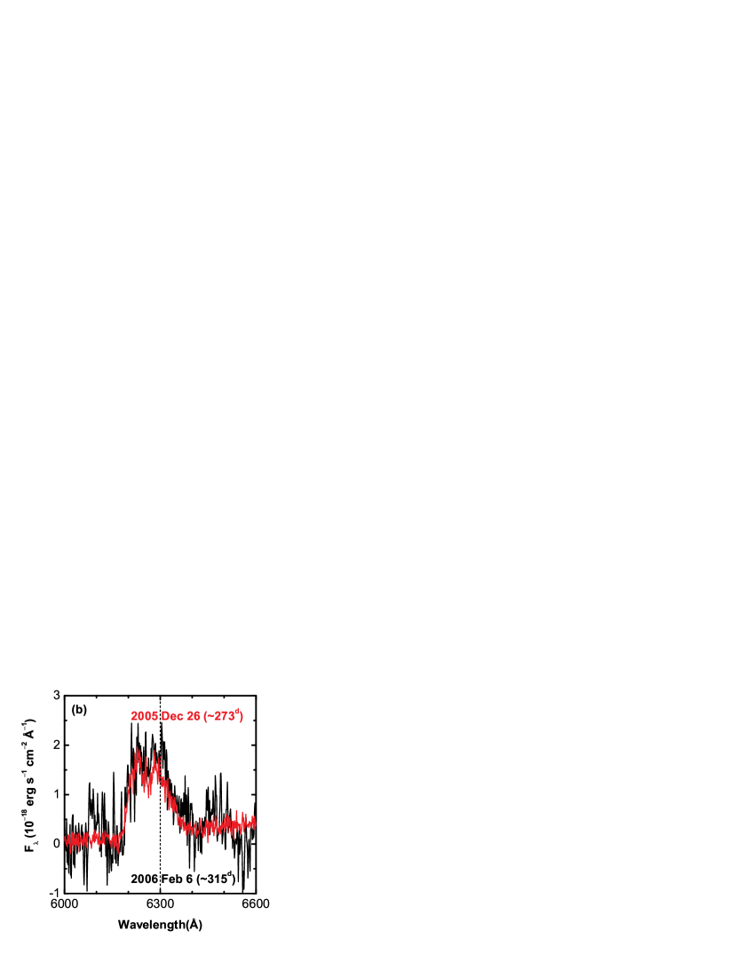
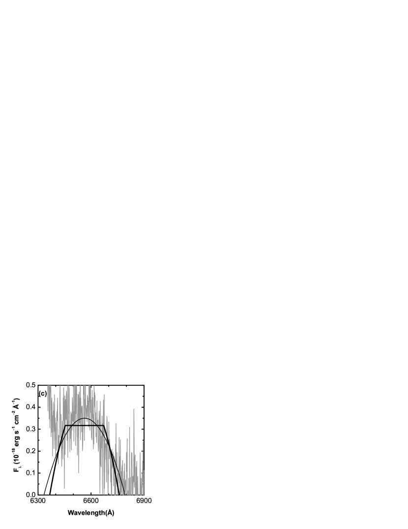
Figure 1.— The reduced spectra of SN 2005bf. The redshift of the host galaxy ($z=0.018913$) is corrected for. The flux of the December spectrum is calibrated using the $R$-band photometry. (a) The spectra at 2005 December 26 (upper) and at 2006 Feb 6 (lower). The flux of the December spectrum is shifted upward by the amount of $3\times 10^{-18}$ erg s^-1 cm^-2 Å^-1 for presentation. (b) The expanded view at 6000 – 6600Å (the [OI] $\lambda\lambda$ 6300, 6363) for the December (red) and the February (black) spectra. The flux of the February spectrum is multiplied by an arbitrary amount for presentation. (c) The expanded view at 6300 – 6900Å of the December spectrum (gray). The parabola fit as the H_α emission is shown for the outermost velocity 10,500 km s^-1 (FWHM $\sim 15,000$ km s^-1; thin black). Also shown is the fit by the parabola with the outermost velocity 9,000 km s^-1 with the central flat part below 5,000 km s^-1 (thick black).

In this paper, we present results from late-phase spectroscopy and photometry of SN 2005bf at $t\sim 273^{\rm d}$ and $315^{\rm d}$. SN 2005bf has clearly entered into the nebular phase, so it is possible to derive information qualitatively different from that derived with the early phase observations. The observed features turn out to be even more peculiar than expected from the early phase observations. We will critically examine some ideas whether they give a view consistently explaining both the previous and the new observations. At the end, we suggest a scenario that SN 2005bf is a birth event of a strongly magnetized neutron star (magnetar) and this central remnant is the heating source – a scenario which could solve the puzzles found by our new observations.

In §2, we describe the observation and data reduction. In §3, the nebular spectra are examined in detail. In §4, we present the light curve connecting the new and previous observations, and discuss a problem brought by the new observations. In §5, we discuss and critically examine possible underlying scenarios. Among the scenarios, we highlight the magnetar scenario in §6, where consequences and implications of this scenario are mentioned. The paper is closed in §7 with conclusions.

2. OBSERVATIONS AND DATA REDUCTION

Spectroscopy and photometry of SN 2005bf have been performed on 2005 December 26 (UT) and on 2006 February 6 with the 8.2 m Subaru telescope equipped with the Faint Object Camera and Spectrograph (FOCAS; Kashikawa et al. 2002). The epochs correspond $t\sim 273^{\rm d}$ and $\sim 315^{\rm d}$. For spectroscopy, we used $0\farcs 8$ width slit and B300 grism, which gave a wavelength coverage of 4700–9000 Å and a spectral resolution of $\simeq 10.7$ Å. The exposure times were 12600 s and 6600 s for 2005 December and 2006 February, respectively. BD +28^∘4211 and G191B2B (Massey et al. 1988; Massey & Gronwall 1990) were also observed for flux calibrations. For photometry, we obtained 180 s exposure images with either $B$- or $R$-band filter on both nights. The derived magnitudes were $B>25.6$ mag and $R=24.4\pm 0.2$ mag on 2005 December 26 and $B>24.6$ mag and $R>24.5$ mag on 2006 February 6. Since we could not recognize SN 2005bf in the $B$-band image on 2005 December 26 and in the $B$- and $R$-band images on 2006 February 6, we adopted $5-\sigma$ background as the upper-limit of the magnitude. We obtained images of standard stars around PG 0942-029 (Landolt 1992) for photometric calibrations.

Figure 1 shows the reduced spectra of SN 2005bf. At 2005 December 26, SN 2005bf was already in a nebular phase, characterized by strong emission lines with almost no continuum. No significant evolution is seen between December 26 and February 6 either in line profiles or line flux ratios, although the low S/N in the February spectrum prevents us from rejecting possible difference in detailed line structures. Spectroscopic features are discussed in §3 in detail.

Figure 2 shows the late phase $B$ (only upper limits) and $R$ magnitudes of SN 2005bf as combined with previously published ones (from Tominaga et al. 2005). The light curve is compared with the $R$-band and the bolometric light curves of SN Ic 1998bw (Patat et al. 2001), and with the $R$-band light curve of SN Ib 1990I (Elmhamdi et al. 2004) corrected for the distance and the reddening to the position of SN 2005bf. Surprisingly enough, SN 2005bf turned out to be extremely faint at the late epochs. The light curve characteristic is further discussed in §4, where we see that the faintness of SN 2005bf at the late epochs is difficult to understand in the context of a conventional supernova emission model.

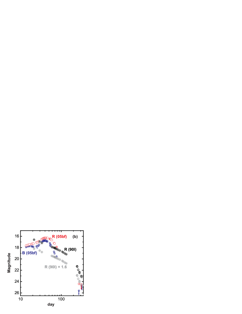
Figure 2.— The $R$-band (red open circles) and $B$-band (blue stars) light curves of SN 2005bf. Time is measured since the explosion, which is assumed to have occurred on 2005 March 28 (Tominaga et al. 2005). The Subaru observation of $R$ at December 26 and upper limits ($B$ at December 26, $R$ and $B$ at February 6) are shown. The early phase data ($<100$ days) are from Tominaga et al. (2005). The light curves are compared with those of SN 1998bw (a: $R$ shown by black open circles, and the bolometric magnitude shown by a black curve; from Patat et al. 2001) and of SN 1990I (b: $R$ shown by black open circles; from Elmhamdi et a. 2004). The magnitudes of SNe 1998bw and 1990I are corrected for the distance modulus and the reddening to the position of SN 2005bf.

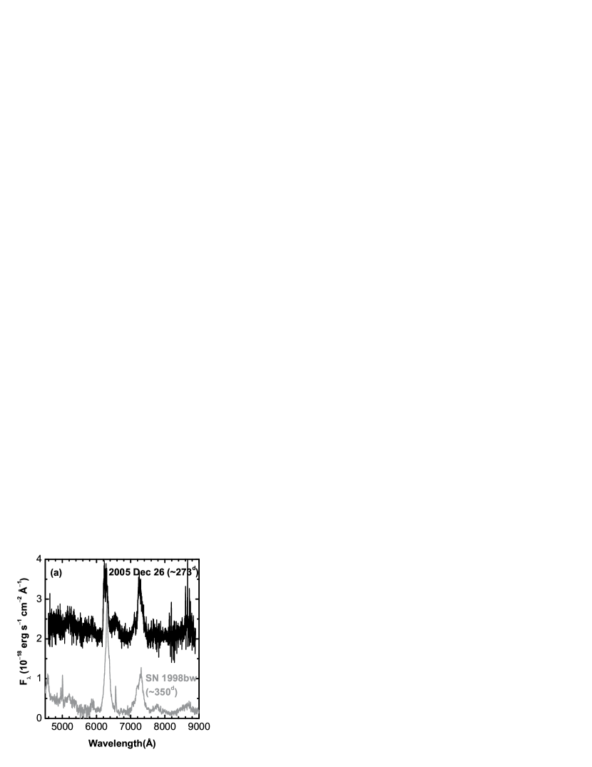
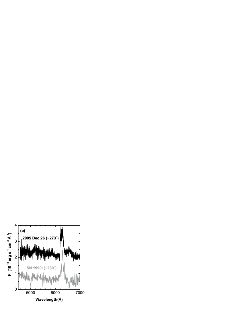
Figure 3.— Comparison of the December spectrum with (a) SN 1998bw and (b) SN 1990I at similar epochs. Flux is shifted artificially for SNe 1998bw and 1990I for presentation. The flux of the December spectrum is shifted upward by the amount of $2\times 10^{-18}$ erg s^-1 cm^-2 Å^-1 for presentation. The redshifts of the host galaxies are corrected for.

3. NEBULAR SPECTRA

3.1. General Features

The reduced spectra show strong emissions at $\sim 6300$Å, $7300$Å, which we interpret as [OI] $\lambda\lambda$6300, 6363 doublet and [CaII] $\lambda$7300 (actually a combination of [CaII] $\lambda\lambda$7291, 7324, and [FeII] $\lambda\lambda$7155, 7172, 7388, and 7452). Other emission features are marginally detected at $\sim 5200$Å (likely a blend of [FeII]) and $\sim 8700$Å(CaII IR and [CI] $\lambda$8727).

A feature at $\sim 6,500$Å is consistent with broad H_α emission (FWHM $\sim 15,000$ km s^-1 measured in the December spectrum). This feature was reported in a spectrum taken at 2005 October 31 ($t\sim 210^{\rm d}$), but the width reported was narrower (FWHM $\sim 3,400$ km s^-1: Soderberg et al. 2005). This feature is marginally detected in our February spectrum, but the shape is uncertain because of the low S/N.

We believe this is the H_α emission. Excessive emission at the red wing of [OI] $\lambda\lambda$6300, 6363 is sometimes observed in SNe Ib/c at relatively early epochs ($t\sim 100^{\rm d}$), and in such a case possible interpretation suggested to date is either [SiI] $\lambda$6527 (e.g., 1997ef: Mazzali et al. 2004) or H_α (e.g., 1991A: Fillipenko 1991, see also Matheson 2001). The detection of this feature at $t\mathrel{\hbox to0.0pt{\lower 4.0pt\hbox{\hskip 1.0pt$\sim$}\hss}\raise 1.0pt\hbox{$>$}}200^{\rm d}$ is not common, but there is at least one another SN showing a similar feature (SN 2004gn, which will be reported elsewhere).

The feature, assuming it is H_α, is either consistent with an emitting sphere with the outer boundary at $v\sim 10,000$ km s^-1 or an emitting shell bound between $v\sim 5,000-10,000$ km s^-1. The velocity at the outer boundary of the emitting H_α is similar to, but smaller than, the velocity of H ($v\sim 13,000$ km s^-1) seen in the spectrum at 2005 Apr 13 ($t\sim 15^{\rm d}$: Anupama et al. 2005; Tominaga et al. 2005). Since this velocity is very large as compared with the center of the ⁵⁶Ni distribution along the line of sight ($v\sim 2,000$ km s^-1: see §§3.2 & 3.3), it is probably difficult to ionize/excite H by the radioactive gamma-rays and resulting UV photons. More likely, the H_α comes from the ejecta decelerated by the weak CSM interaction. In any case, the detection of the high-velocity H_α supports the existence of the thin H envelope suggested by Anupama et al. (2005) and Tominaga et al. (2005). The line center of the H_α emission is consistent with the rest wavelength (Fig. 1), but the strong contamination in the blue wing by the [OI] makes the judgment difficult.

No strong emission is seen at [OI] $\lambda 5577$. The line ratio L([OI] $\lambda\lambda 6300,6363$: ¹D₂ $\to$ ³P)/L([OI] $\lambda 5577$: ¹S₀ $\to$ ¹D₂) is related to the electron number density ($n_{\rm e}$ [cm^-3]) and the electron temperature ($T_{3}\equiv T_{\rm e}/1000{\rm K}$) as follows (under the usual assumption that the ¹D₂ and ¹S₀ levels are populated by thermal electron collisions).

$$\frac{L_{6300+6363}}{L_{5577}}=7.2\beta_{6300}\frac{1+6.6\times 10^{-9}n_{\rm e}T_{3}^{0.02}}{1+1.6\times 10^{-6}n_{\rm e}T_{3}^{0.03}}e^{\frac{25.83}{T_{3}}}\ ,$$ (1)

where $\beta_{6300}$ is the Sobolev escape probability of the [OI] $\lambda 6300$ and about unity at the epoch of interest in the present paper. The expression is derived by solving rate equations for a simplified OI atomic model. It is correct to the first order in $n_{\rm e}$ and in the exponential term for $T_{\rm e}$. The form is somewhat different from that in Houck & Fransson (1996), but these two expressions are consistent with each other in the density and temperature ranges of interest here ($n_{\rm e}\sim 10^{6}-10^{10}$ cm^-3 and $T_{3}\sim 1-10$). Taking the rough estimate L([OI] $\lambda\lambda 6300,6363$)/L([OI] $\lambda 5577$) $\mathrel{\hbox to0.0pt{\lower 4.0pt\hbox{\hskip 1.0pt$\sim$}\hss}\raise 1.0pt\hbox{$>$}}10$, the emitting region should be at relatively low temperature ($T_{3}\mathrel{\hbox to0.0pt{\lower 4.0pt\hbox{\hskip 1.0pt$\sim$}\hss}\raise 1.0pt\hbox{$<$}}4$, for the high density limit) and/or at low electron density ($n_{\rm e}\mathrel{\hbox to0.0pt{\lower 4.0pt\hbox{\hskip 1.0pt$\sim$}\hss}\raise 1.0pt\hbox{$<$}}5\times 10^{6}$ cm^-3, if $T_{3}=10$).

The low density is supported from the large ratio of [CaII] $\lambda$7300 to CaII IR. The OI $\lambda$7774 is weak, further supporting the low density. It also suggests that ionization is low. SN 2005bf at $t\sim 300^{\rm d}$ belongs to the low density end of a typical condition seen in SNe Ibc at nebular phases with $n_{\rm e}\sim 10^{6}-10^{9}$ cm^-3 (see, e.g., Fransson & Chavalier 1989).

Figure 3 shows comparison of the December 26 spectrum with the spectra of SNe 1998bw and 1990I at similar epochs . Note that the flux is arbitrarily shifted for SNe 1998bw and 1990I for presentation. Despite the large difference in the luminosity (Fig. 2) and possibly in the line shapes and some line ratios, the overall features look similar among these objects. The [OI] $\lambda$6300/[CaII] $\lambda$7300 ratio in SN 2005bf is smaller than that of SN 1998bw. The oxygen core mass increases very sensitively as a function of $M_{\rm ms}$, while the explosively synthesized Ca does not. The smaller [OI]/[CaII] ratio thus indicates that the progenitor of SN 2005bf is less massive than SN 1998bw, i.e., $M_{\rm ms}<40M_{\odot}$. (See, e.g., Nakamura et al. 2001b and Nomoto et al. 2006 for the supernova yields. See Fransson & Chevalier 1987, 1989 for the theoretical [OI]/[CaII] ratios for the specific cases of $15M_{\odot}$ and $25M_{\odot}$ progenitor models. See also Maeda et al. 2007 for discussion on the [OI]/[CaII] ratio in other SNe Ib/c.)

3.2. Line Profiles and Blueshift

Figure 4.— Line profiles in velocity space (a minus sign for blueshift). The centers of the line are 6300 ([OI]), 7150 (FeII), and 7300Å([CaII]). The velocity toward us is marked for 0 km s^-1 (black dashed) and for 2,000 km s^-1 (gray dashed).

The observed line profiles and positions are very unique. Figure 4 shows line profiles around 6300, 7150, and 7300Å, which we attribute to [OI] $\lambda\lambda$6300, 6363, [FeII] $\lambda$7155, and [CaII] $\lambda\lambda$7291, 7324. The line profiles are shown in velocity relative to 6300, 7150, 7300Å (after correcting for the host’s redshift). All these lines show similar amount of blueshift relative to the rest wavelength ($\sim 1,500-2,000$ km s^-1).

The doubly-peaked profile of the [OI] is especially unique. This is clearly seen in the December spectrum, and is consistent with the low S/N February spectrum. Also, this feature is seen in another spectrum at a similar epoch taken independently (M. Modjaz, private communication). Thus, this peculiar line shape should be real. Note this is different from the doubly-peaked [OI] profile seen in SN 2003jd (Mazzali et al. 2005). In the case of SN 2003jd, it was basically symmetric with respect to the rest wavelength (i.e., no velocity shift), so that it was most naturally interpreted as oxygen distributed in a disk viewed from the equator (Maeda et al. 2002).

By comparing these three lines, we can obtain insight on the distribution of materials. Between the two peaks in the [OI] emission, the [CaII] emits strongly, and the [FeII] is even more narrowly centered. The simplest interpretation is that the elements have layered distribution, i.e., Fe at the center of the emitting region ($v\sim 2,000$ km s^-1), which is surrounded by Ca, then by O.

3.3. Spectrum Synthesis

Table 2Spectrum Models

Model	$M_{\rm ejneb}$	$V$	$dV$	C	O	Na	Ca	56Ni	$T_{\rm e}$	log $n_{\rm e}$	$\tau_{\rm abs}$
A	0.12	3,500	1,800	0.023	0.07	3.6E-5	7.2E-5	0.024	5,100	6.4	0
B	0.34	5,000	0	0.068	0.21	1.0E-4	2.0E-4	0.056	5,200	6.3	2 (67% absorbed)

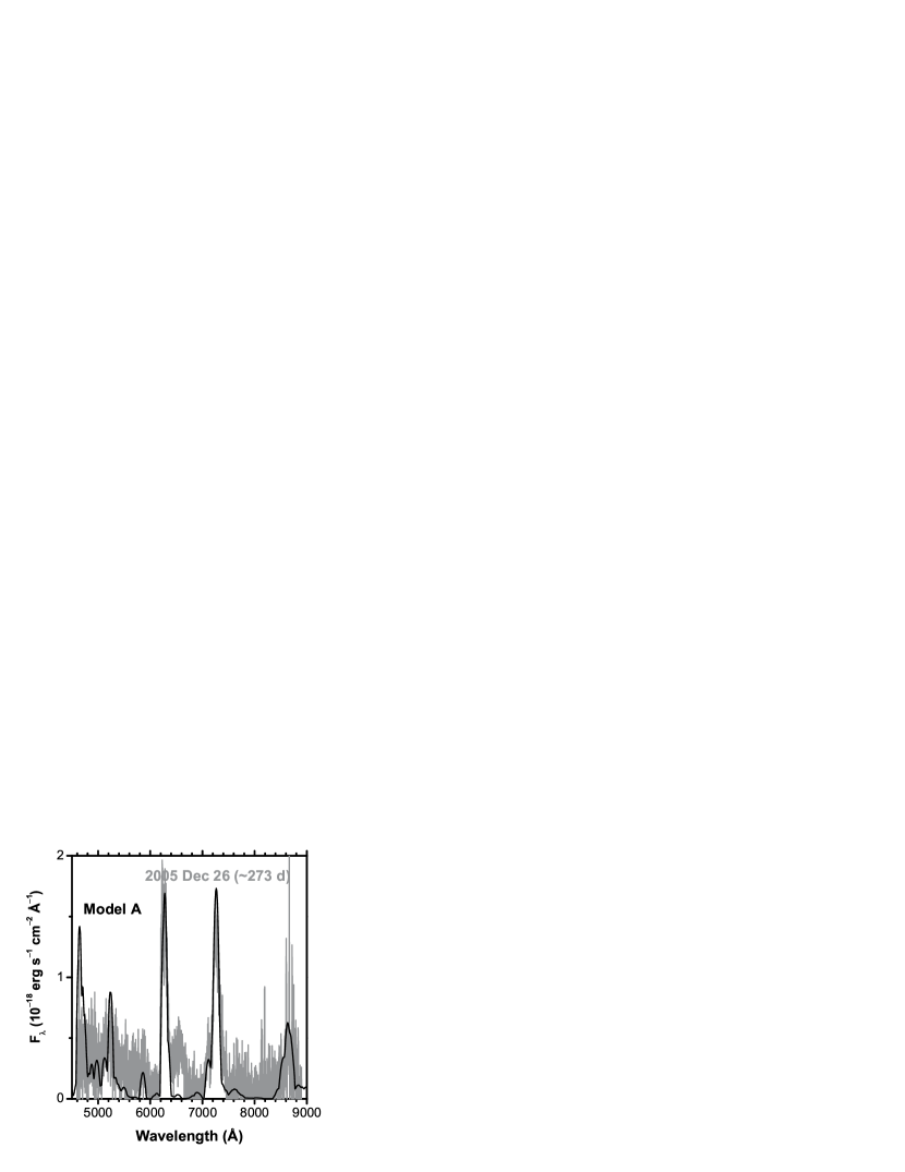
Figure 5.— Model spectra at $t=270^{\rm d}$ (black solid), as compared with the December 26 spectrum (gray). For Model B, the original unabsorbed spectrum is also shown (dotted). See Table 2 for model parameters. The distance modulus $\mu=34.5$ and $E(B-V)=0.045$ are adopted.

The similarity of the nebular spectra (Fig. 3) indicates that $n_{\rm e}$ and $T_{\rm e}$ are similar for SNe 2005bf, 1998bw, and 1990I at similar epochs. We have performed one-zone nebular spectrum synthesis computations. Following the ⁵⁶Ni $\to$ ⁵⁶Co $\to$ ⁵⁶Fe decay chain as a heating source, the code computes gamma-ray deposition in a uniform nebula by the Monte-Carlo radiation transport Method. Positrons from the decays are assumed to be trapped completely (see §4.1). Positrons become a predominant heating source after the optical depth to the gamma-rays drops below $\sim 0.035$, following the density decrease. Ionization and NLTE thermal balance are solved according to the prescription given by Ruiz-Lapuente & Lucy (1992). See Mazzali et al. (2001) and Maeda et al. (2006a) for details. Hereafter, we use the subscript ”neb” for the values derived by modeling the nebular phase observations, i.e., $M_{\rm ej,neb}$, $M$(⁵⁶Ni)_neb, and so on (see Table 1).

In the present models, we do not introduce He in the nebula. If the ejecta are heated totally by positrons, adding He does not affect the masses of the other elements derived in the spectrum synthesis. In this case, He has virtually nothing to do with both heating and cooling of the ejecta. On the other hand, if the ejecta are heated predominantly by gamma-rays, the situation is different. Increasing He mass fraction leads to lowering mass fractions of the other elements including ⁵⁶Ni. However, to reproduce the observed total luminosity, reducing the fraction of ⁵⁶Ni should be compensated by increasing the ejecta mass to absorb gamma-rays more effectively. Thus, the mass of the emitting materials ($M_{\rm ej,neb}$) derived without He is the lower limit. Likewise, the mass of each element, as well as that of ⁵⁶Ni, obtained without He is the upper limit for the mass of each element, because the mass fraction for each element should be lower.

There are two possible ways to reproduce the blueshift in emission lines. One is the kinematical off-set in the distribution of the emitting materials (Model A: §3.3.1), and the other is the self-absorption within the ejecta reducing the contribution of light coming from the far side of the ejecta (Model B: §3.3.2). Figures 5 and 6 show the comparison between the model spectra and the December spectrum. Model parameters are listed in Table 2. Because of the one-zone treatment in the spectrum synthesis, we are not concerned with the detailed line profiles.

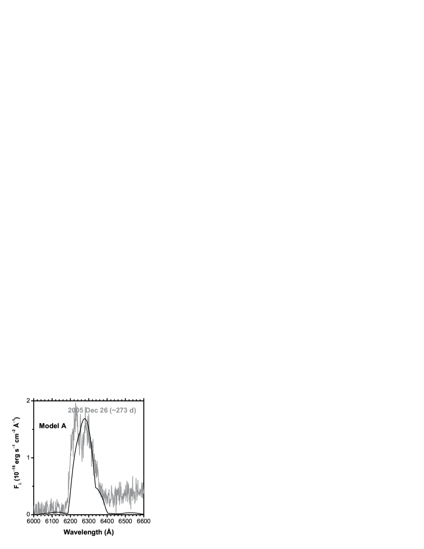
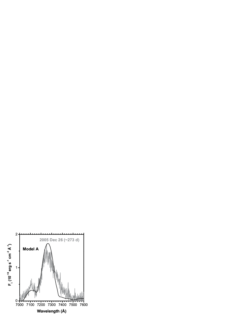
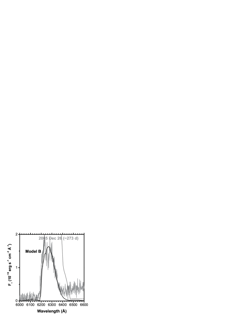
Figure 6.— Same with Figure 5, but for the [OI] $\lambda\lambda$6300, 6363 and for the [CaII] $\lambda$7300 + [FeII] $\lambda$7150.

3.3.1 Unipolar Blob: Model A

In Model A, we neglect the optical radiation transport effect in the nebula, except for the optical depth effect within a line in the Sobolev approximation. As the observed spectrum shows blueshift relative to the expected line positions (Fig. 4: see also §3.2), we artificially shift the model spectrum blueward by $1,800$ km s^-1. The blueshift in this model is totally attributed to the kinematical distribution of the emitting materials (see e.g., Motohara et al. 2006). This is discussed later in this section.

In Model A, $M_{\rm ej,neb}\sim 0.12M_{\odot}$ and $M$(⁵⁶Ni)${}_{\rm neb}\sim 0.024M_{\odot}$. These values are only $\sim 2\%$ and $8\%$ of $M_{\rm ej,peak}$ and $M$(⁵⁶Ni)_peak, respectively. Contrary, the same fractions are $\sim 25-50$% ($M_{\rm ej}$) and $\sim 100$% ($M$(⁵⁶Ni)) for SN 1998bw (Mazzali et al. 2001). These values in Mazzali et al. (2001) are consistent with the expectation that in late phases we look into the ⁵⁶Ni-rich region. In this sense, $M_{\rm ej,neb}$ and $M$(⁵⁶Ni)_neb for SN 2005bf are too small to be compared with $M_{\rm ej,peak}$ and $M$(⁵⁶Ni)_peak.

The electron density derived for SN 2005bf is similar to that for SN 1998bw at similar epochs (Mazzali et al. 2001). We find that introducing clumpy structures in SN 2005bf does not help. If the filling factor is smaller, then the oxygen mass should be even smaller to fit the [OI]$\lambda 6300$ luminosity. Derived $n_{\rm e}$ (Table 2) is close to the critical density for the [OI]$\lambda 6300$ emission, thus increasing $n_{\rm e}$ results in increasing the line emissivity per neutral oxygen.

The CaII IR profile suggests a strong contribution from [CI] $\lambda$8727 in the red. If this is true, then we need relatively large mass ratio $\sim 0.35$ between C and O. This is consistent with the ratio for $M_{\rm ms}\mathrel{\hbox to0.0pt{\lower 4.0pt\hbox{\hskip 1.0pt$\sim$}\hss}\raise 1.0pt\hbox{$<$}}20M_{\odot}$ (e.g., Nomoto et al. 2006).

Now we turn to the detailed element distribution. Figure 7 shows toy models to fit the line profiles, computed by assuming that the flux density is simply proportional to the density of homogeneous matter, and by artificially shifting the flux. As long as only the line profiles are concerned, various geometry can reproduce the observation. The blue shift suggests that a blob (or a jet) of ⁵⁶Ni is ejected, and its center-of-mass velocity is $v\mathrel{\hbox to0.0pt{\lower 4.0pt\hbox{\hskip 1.0pt$\sim$}\hss}\raise 1.0pt\hbox{$>$}}2,000$ km s^-1. Also, more centrally (but off-set from the SN rest) concentrated distribution of heavier elements yields a good fit to their narrower line profiles. If the viewing direction ($\theta$ measured from the pole) is close to the pole (Case A1: $\theta\sim 15^{\rm o}$), then the distribution of the oxygen should be more elongated to the same direction to explain the doubly-peaked [OI]. If $\theta$ is large (Case A2: $\theta\sim 75^{\rm o}$), on the other hand, the torus-like structure of oxygen-rich materials is necessary (Maeda et al. 2002; Mazzali et al. 2005). It should be interesting to examine in the future if these distributions can be reproduced by unipolar supernova explosion models (Hungerford, Fryer, & Rockefeller 2005).

In sum, in Model A, the spectrum of SN 2005bf at $t\sim 270^{\rm d}$ is explained by the ejection of a blob with $M_{\rm ej,neb}\sim 0.12M_{\odot}$ and $M$(⁵⁶Ni)_neb $\sim 0.024M_{\odot}$. The blob is centered at $v\mathrel{\hbox to0.0pt{\lower 4.0pt\hbox{\hskip 1.0pt$\sim$}\hss}\raise 1.0pt\hbox{$>$}}2,000$ km s^-1, distributed in $v\sim-2,000-\sim 5,000$ km s^-1 (Case A1) or $v\sim 0-\sim 8,000$ km s^-1 (Case A2) depending on $\theta$ (Fig. 7).

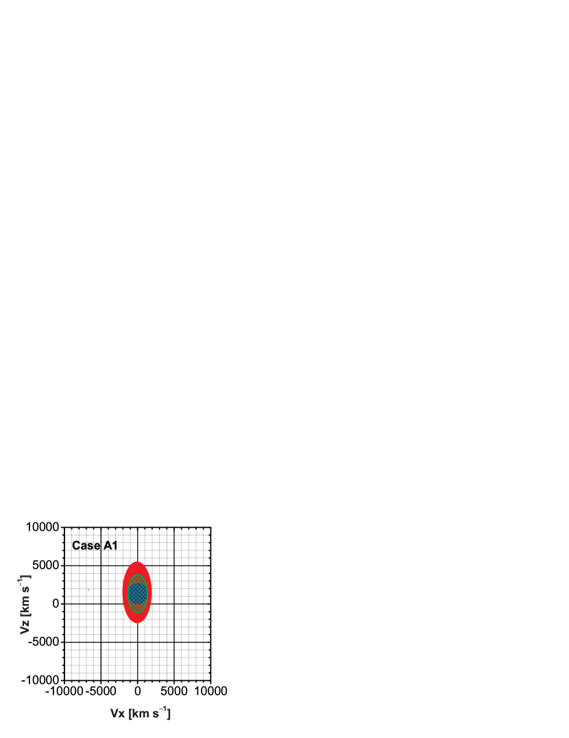
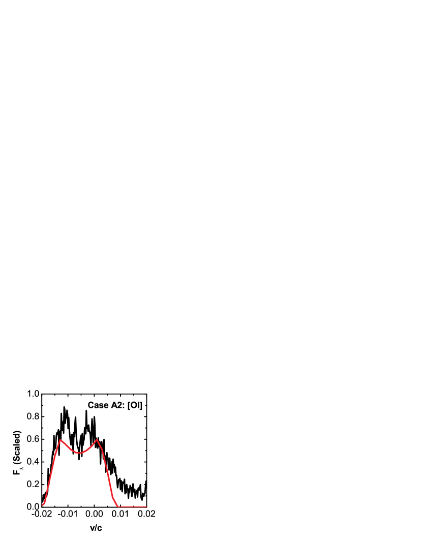
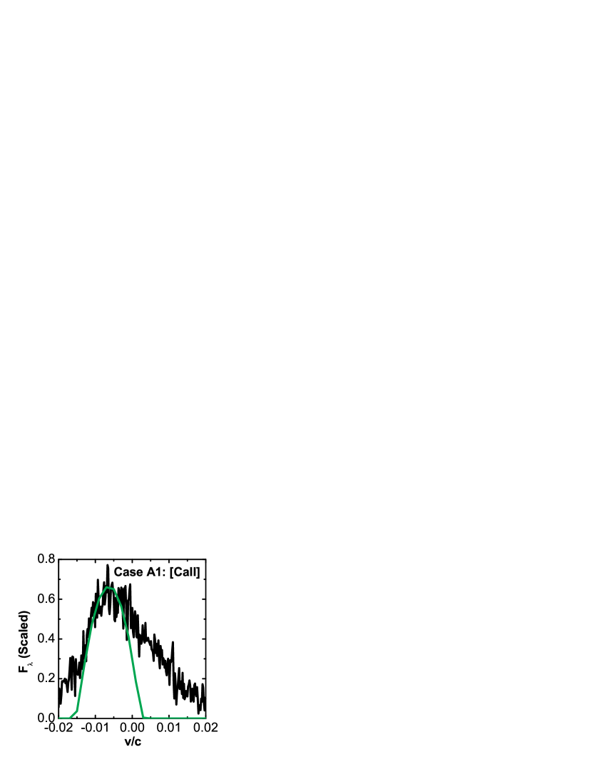
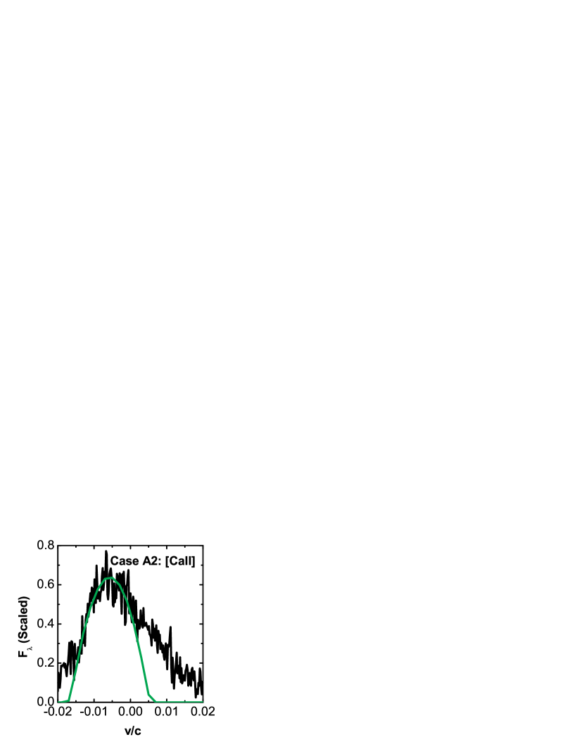
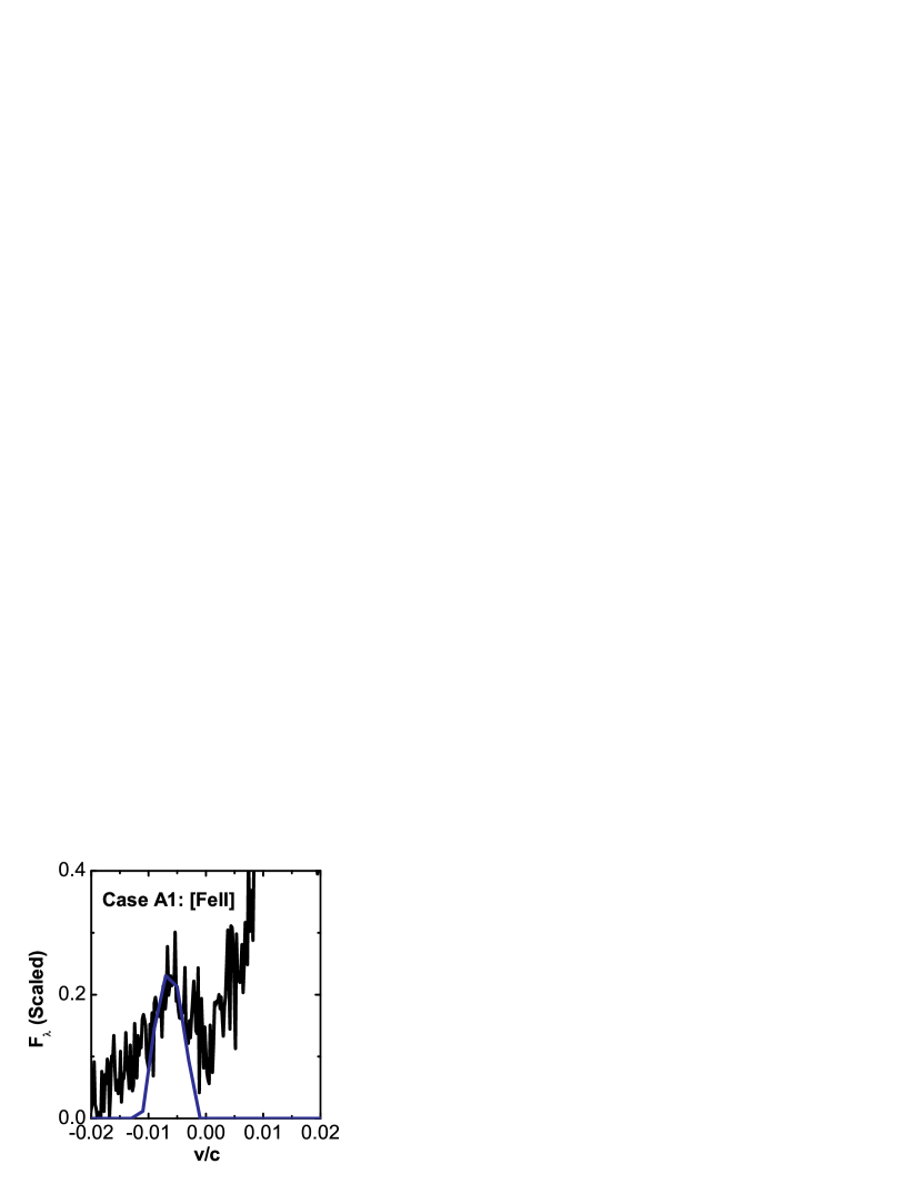
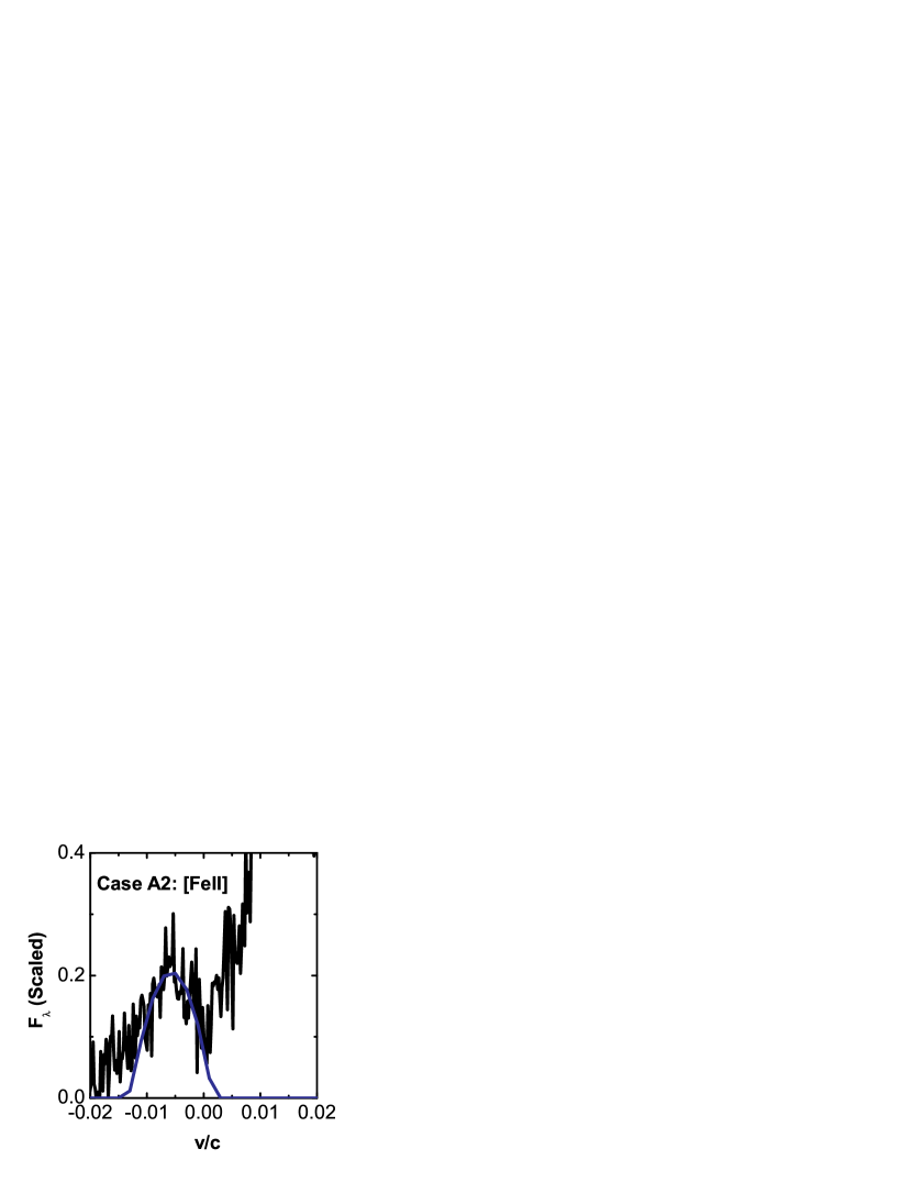
Figure 7.— Simple model fits to the line profiles. (a, Case A1: left panels) The blob model viewed at $\theta\sim 15^{\rm o}$ from the pole (i.e., $+V_{z}$-direction). The distribution is shown for O (red), Ca (green), and Fe (blue). The expected line profiles are shown for the [OI] $\lambda\lambda$6300, 6363 (red), [CaII] $\lambda\lambda$7291, 7324 (green), and [FeII] $\lambda$7155 (blue) (from top to bottom). (b, Case A2: right panels) The blob model viewed at $\theta\sim 75^{\rm o}$ from the pole (i.e., $+V_{x}$-direction).

3.3.2 Self-Absorption: Model B

Another interpretation is also possible for the blueshift of the emission lines. Figures 2 and 3 show the similarity between SNe 2005bf and 1990I in the light curve shape except for the peak at $t\sim 40^{\rm d}$, and in the nebular spectra. The early phase spectra could also be similar (A. Elmhamdi, private communication). The similarity may suggest that similar physical conditions could apply for these SNe.

SN 1990I experienced the onset of blueshift in emission lines and accelerated fading in optical luminosity almost simultaneously (e.g., Elmhamdi et al. 2004). These are interpreted as the onset of dust formation and the self-absorption of optical light by the dust particles. Elmhamdi et al. (2004) constrained the fraction of the absorbed optical light $\sim 50\%$ at $t\sim 300^{\rm d}$ for SN 1990I.

In Model B, we assume that the similar fraction of the optical light experiences the absorption within the ejecta. We take the absorbed fraction to be $\sim 70\%$ (Table 2). In the spectrum synthesis for Model B, the optical light is dimmed as

$$I=I_{0}\exp(-\kappa_{\rm abs}\rho l)\ ,$$ (2)

where $I_{0}$ is the original intensity without absorption, and $l$ is the path length for each photon until escaping the nebula. The absorption opacity $\kappa_{\rm abs}$ is taken to be constant through the ejecta. The value of $\kappa_{\rm abs}$ is set by the requirement that the emergent luminosity is $\sim 30\%$ of the original luminosity.

For the larger amount of absorption, the original luminosity should be larger to reproduce the observed luminosity. Accordingly, $M_{\rm ej,neb}$ and the mass of each element are larger in Model B than in Model A, as seen in Table 2.

At the same time, the absorption dilutes the optical light from the far side selectively, thus causing the blueshift of the emission lines. Figure 6 shows that the blueshift similar to the observed one can be obtained although no kinematical off-set is assumed in Model B. The synthetic spectrum is bluer than observed for the [FeII] $\lambda$7150 and [CaII] $\lambda$7300, indicating that these elements are more centrally concentrated than oxygen, as is required in Model A. The absorption in the uniform sphere does not itself reproduce the doubly-peaked [OI] $\lambda\lambda$6300, 6363 doublet. The distribution of oxygen should be as shown in Figure 7, except for the center of the distribution which should be at the zero-velocity in Model B.

In Model B, $M_{\rm ej,neb}\sim 0.34M_{\odot}$ and $M$(⁵⁶Ni)_neb $\sim 0.056M_{\odot}$. The velocity of the outer edge of the emitting blob is $v\sim 5,000$ km s^-1, which is similar to that in Model A.

4. LATE TIME LIGHT CURVE

4.1. General Remarks

The magnitude difference between the second peak ($t\sim 40^{\rm d}$) and the late epoch ($t\sim 270^{\rm d}$) is $\Delta B>8.9$ mag and $\Delta R\sim 8.1$ mag. These are at least 2 magnitudes larger than seen in SNe 1998bw and 1990I (Fig. 2). Since the peak-to-tail luminosity difference is similar for different SNe Ib/c (e.g., Patat et la. 2001; Elmhamdi et al. 2004; Tomita et al. 2006; Richardson, Branch, & Baron 2006), the very large difference in SN 2005bf is a unique property.

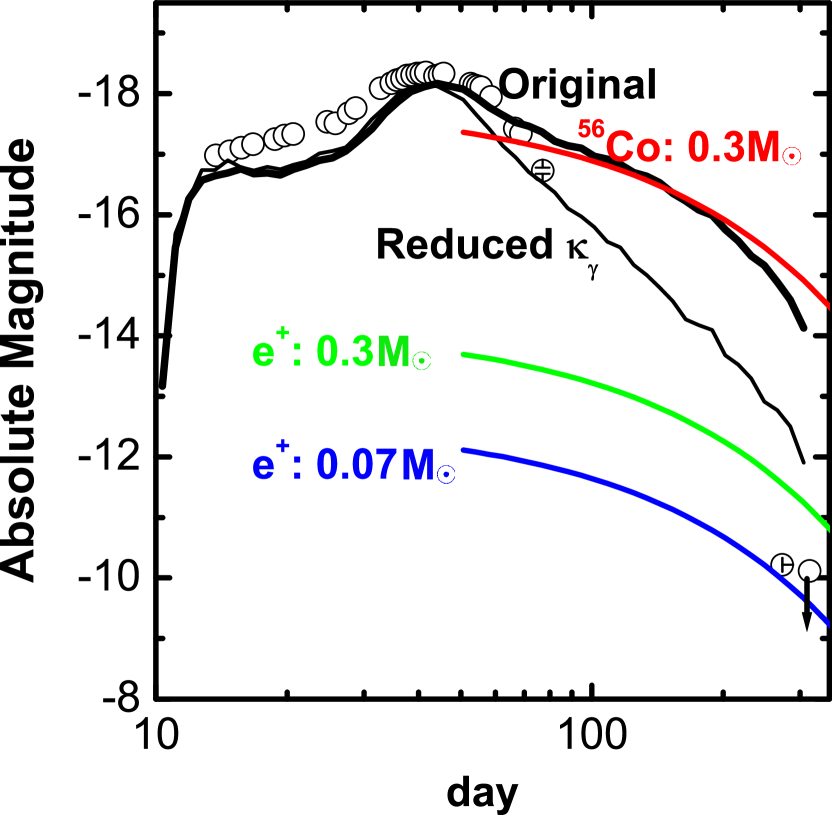
Figure 8.— The $R$-band light curve of SN 2005bf (circles), as compared with the model curves (black curves). The ejecta model is adopted from Tominaga et al. (2005), in which $M_{\rm ej,peak}=7.3M_{\odot}$, $E_{{\rm peak},51}=1.3$, and $M$(⁵⁶Ni)_peak $=0.32M_{\odot}$. Two models are shown (without/with reducing gamma ray opacity shown by thick/thin solid curve). Also shown is the energy generation rate by gamma-rays and positrons from $0.3M_{\odot}$ of ⁵⁶Co (red), and the energy generation rate only by positrons from $0.3M_{\odot}$ (green) and $0.07M_{\odot}$ (blue) of ⁵⁶Co.

Figure 8 shows the comparison between the $R$-band light curve of SN 2005bf and synthetic bolometric curves computed using the ejecta model of Tominaga et al. (2005) with $M_{\rm ej,peak}=7.3M_{\odot}$, $E_{{\rm peak},51}=1.3$ and $M$(⁵⁶Ni)_peak $=0.32M_{\odot}$. The light curves are computed by the Monte Carlo Radiation transport code described in Maeda et al. (2003) (see also Cappellaro et al. 1997). We adopt the absorptive opacity $\kappa_{\gamma}=0.025$ cm² g^-1 for the gray gamma ray transport (see e.g., Maeda 2006c). The optical opacity prescription is similar to Tominaga et al. (2005): we assume that contribution from electron scatterings is equal to that from the line opacity (for the prescription for the line opacity, see Tominaga et al. 2005). This is largely consistent with the electron scattering opacity found in Tominaga et al. (2005) within a factor of two. Figure 8 shows that our synthetic light curve is consistent with the model curve computed by Tominaga et al. (2005). Also shown is the synthetic light curve computed using the reduced gamma ray opacity ($\kappa_{\gamma}=0.001$ cm² g^-1) at $v<5,400$ km s^-1 as examined in Tominaga et al. (2005).

The $R$-band magnitude at $t\sim 270^{\rm d}$ is fainter than the bolometric magnitude expected from the model of Tominaga et al. (2005) by $\sim 5$ mag (!) for the ”brighter” expectation (without reducing $\kappa_{\gamma}$) or $\sim 3$ mag even for the ”fainter” expectation (with reducing $\kappa_{\gamma}$). Since the $R$ magnitude is usually a good tracer of the bolometric magnitude in SNe Ib/c (see Fig. 2 for SN 1998bw), this large discrepancy is very odd and difficult to understand.

Such a very rapid fading has never been observed in SNe Ib/c. The light curve of typical SNe Ib/c is reproduced by the energy input from gamma-rays and positrons produced in the radioactive decay chain ⁵⁶Ni $\to$ ⁵⁶Co $\to$ ⁵⁶Fe. However, the newly observed light curve points of SN 2005bf turn out to be difficult to fit into this context. In late phases, the bolometric luminosity is equal to the energy of gamma-rays absorbed in the ejecta per unit time, as the radiation transfer effect is negligibly small. The gamma-ray optical depth can be estimated by

$$\tau_{\gamma}\sim 1000\times\frac{(M_{\rm ej}/M_{\odot})^{2}}{E_{51}}\times\left(\frac{t}{{\rm day}}\right)^{-2}$$ (3)

(see e.g., Maeda et al. 2003). The model of Tominaga et al. (2005) or Folatelli et al. (2006) predict $\tau_{\gamma}\sim 0.5$ at $t=300^{\rm d}$. For comparison, $\tau_{\gamma}\sim 0.02-0.06$ for SN 1998bw at $t=300^{\rm d}$ ($M_{\rm ej}\sim 10M_{\odot}$, $E_{51}\sim 20-50$: Maeda, Mazzali, & Nomoto 2006b; Nakamura et al. 2001a). Then, the peak-to-tail magnitude difference must be smaller in SN 2005bf than SNe 1998bw, which is inconsistent with what we have observed.

Even more problematic is the fact that SN 2005bf in the late phase is even fainter than the lower limit set by the ⁵⁶Co heating model. Positrons emitted from the ⁵⁶Co decay produce energy at a rate $L_{e^{+}}$:

$$L_{e^{+}}=4.8\times 10^{41}\left(\frac{M(^{56}{\rm Ni})}{M_{\odot}}\right)\exp{\left({-\frac{t}{113\ {\rm day}}}\right)}\ {\rm erg}\ {\rm s}^{-1}\ .$$ (4)

The positrons’ mean free path is on the order of the gyroradius $r_{\rm gyr}$, which is

$$r_{\rm gyr} = \frac{\sqrt{2m_{e}K}c}{eB}$$ (5)

$$\sim 3.4\times 10^{3}\ {\rm cm}\sqrt{\frac{K}{1\ {\rm MeV}}}\left(\frac{B_{\rm mag}}{1\ {\rm gauss}}\right)^{-1}\ .$$

Here $m_{e}$, $e$, $K$ are the mass, charge, and energy of the positron, $B_{\rm mag}$ is the strength of the magnetic field, and $c$ is the speed of light (all expressed in CGS-Gauss unit). A typical radius of the emitting supernova nebula is $\sim 10^{15}$ cm at $t=300^{\rm d}$ with $v\sim 3,000$ km s^-1. Since the positrons’ mean free path is many orders of magnitude smaller than the size of the nebula, all the positrons can be assumed to be trapped in the ejecta (at least in the absence of well aligned magnetic fields: see Milne, The, & Leising 2001). This sets the lower limit of the bolometric luminosity for given $M$(⁵⁶Ni).

It is seen from Figure 8 that the $R$-band and $B$-band magnitudes at $t\sim 270^{\rm d}$ are fainter than $L_{e^{+}}$ expected from $M$(⁵⁶Ni)_peak $\sim 0.3M_{\odot}$. Actually, the $R$ magnitude, assuming this is equal to the bolometric magnitude, is consistent with positron energy input from $0.08M_{\odot}$ of ⁵⁶Ni according to equation (4). Thus, we set the strict upper limit $M$(⁵⁶Ni)_neb $\mathrel{\hbox to0.0pt{\lower 4.0pt\hbox{\hskip 1.0pt$\sim$}\hss}\raise 1.0pt\hbox{$<$}}0.08M_{\odot}$. Since this input power has nothing to do with the gamma ray transport, reducing $\kappa_{\gamma}$ (Tominaga et al. 2005; Folatelli et al. 2006) does not help solve the discrepancy.

4.2. Contribution from the Blob

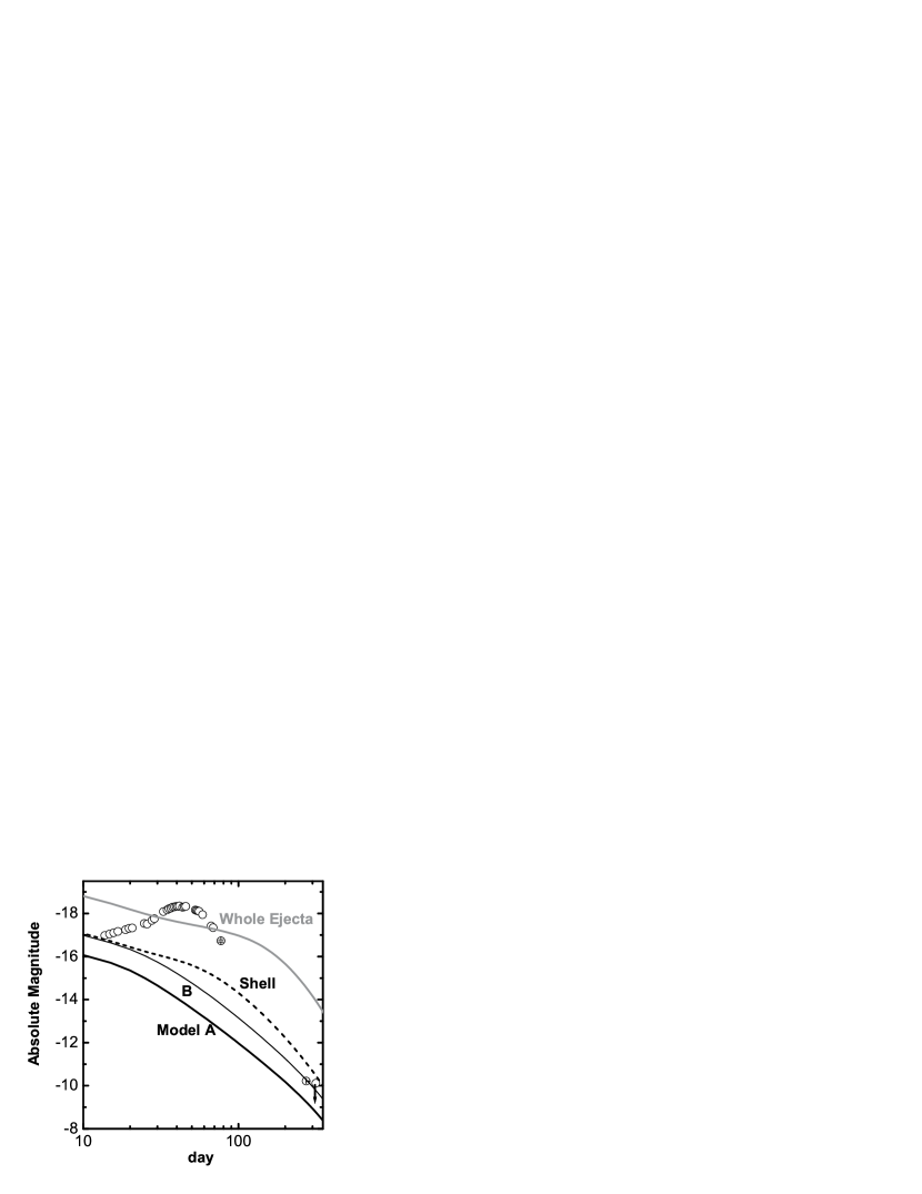
Figure 9.— Light Curve Analysis. The expected deposition luminosity is shown for the whole ejecta (gray solid; $M_{\rm ej,peak}=7.3M_{\odot}$, $E_{{\rm peak},51}=1.3$, and $M$(⁵⁶Ni)_peak $=0.3M_{\odot}$), and for the ⁵⁶Ni-rich shell (dashed; $M_{\rm ej}=2M_{\odot}$, $v=3,900$ km s^-1, and $M$(⁵⁶Ni) $=0.06M_{\odot}$) for the model of Tominaga et al. (2005). Also shown is the deposition luminosity expected for the blob derived from the nebular spectrum, i.e., models A (thick curve) and B (thin curve).

As discussed in §3, the late phase spectra of SN 2005bf are dominated by the emission from a low mass blob with $M_{\rm ej,neb}\sim 0.1-0.4M_{\odot}$ and $M$(⁵⁶Ni)_neb $\sim 0.02-0.06M_{\odot}$. The blob is either ejected with the central velocity $v\sim 2,000$ km s^-1 (if viewed from the pole) – $\sim 5,000$ km s^-1 (if viewed $\sim 75^{\rm o}$ away from the pole), or it suffers from the absorption within the ejecta like SN 1990I. In either case, the emitting materials are distributed up to $v\sim 5,000-8,000$ km s^-1 (§3).

A contribution of the blob component to the light curve is estimated in Figure 9. Taking $M_{\rm ej,neb}$, $E_{{\rm neb},51}$, and $M$(⁵⁶Ni)_neb from Table 1, we use equations (1 – 3) of Maeda et al. (2003) with the modification to include contribution from the ⁵⁶Ni $\to$ ⁵⁶Co decay. In Model B, the luminosity in the nebular epochs ($t\sim 300^{\rm d}$) should be further decreased by $\sim 70\%$ ($\sim 1$ mag) from the curve in Figure 9 to take into account the self-absorption.

It is seen that the energy deposition curve expected from this blob (both models A and B) roughly connects the first peak ($t\sim 20^{\rm d}$) and the late Subaru points ($t\sim 300^{\rm d}$). That is to say, the optical output from SN 2005bf was dominated by this blob component in the earliest and the late epochs, while around the main peak ($t\sim 40^{\rm d}$) the emission from the whole ejecta made the predominant contribution.

Also shown in Figure 9 is the deposition curve expected from the ⁵⁶Ni-rich shell ($3,900$ km s^-1 $<v<$ $5,400$ km s^-1) of Tominaga et al. (2005). The shell has the mass $\sim 2M_{\odot}$ in which $M$(⁵⁶Ni) $\sim 0.06M_{\odot}$. Interestingly, the curve expected from the shell is similar to the blob contribution derived by the nebular spectra. The similar amount of ⁵⁶Ni and the similar velocity between the blob and their shell suggest that what Tominaga et al. (2005) attributed to the shell is actually the blob we derived in this study. However, the total mass of the blob ($M_{\rm ej,neb}\mathrel{\hbox to0.0pt{\lower 4.0pt\hbox{\hskip 1.0pt$\sim$}\hss}\raise 1.0pt\hbox{$<$}}0.4M_{\odot}$) is smaller than what they derived ($\sim 2M_{\odot}$).

Possibly, detailed (2D/3D) ejecta structure and/or the optical opacity prescription affect the mass estimate. These effects are more important in the early phase modeling, since in the early phases only a small fraction of the ejecta is seen and the optical transport effect is strong.

5. DISCUSSION

The late phase data presented in this paper add the following peculiarities to SN 2005bf. (1) It is extremely faint at late phases. (2) Line emissions are blueshifted by $\sim 1,500-2,000$ km s^-1.

The extreme faintness needs special condition (§4). To explain the faintness, there are at least four possibilities.

• The ejecta are much more transparent to gamma-rays and even to positrons than in other SNe.

• The fraction of radiation output in the optical range is extremely small ($\sim 1$ %).

• $M$(⁵⁶Ni) decreases with time, from $M$(⁵⁶Ni)_peak $\sim 0.3M_{\odot}$ at $t\sim 40^{\rm d}$ to $M$(⁵⁶Ni)_neb $\mathrel{\hbox to0.0pt{\lower 4.0pt\hbox{\hskip 1.0pt$\sim$}\hss}\raise 1.0pt\hbox{$<$}}0.1M_{\odot}$ at $t\sim 270^{\rm d}$.

• The peak ($t\sim 40^{\rm d}$), at least, was not powered by the ⁵⁶Ni decay chain.

In this section, we discuss these possible interpretations.

5.1. Gamma-ray and Positron escape?

The drop of the light curve was already observed between $t\sim 40^{\rm d}$ and $\sim 80^{\rm d}$. It was suggested that it could be explained by assuming the reduced gamma-ray opacity $\kappa_{\gamma}$ (Tominaga et al. 2005; Folatelli et al. 2006). This is possible for the period $t\sim 40^{\rm d}-80^{\rm d}$, but we show in the following that this is unlikely to work at the late epochs ($t\sim 300^{\rm d}$).

They argued that the reduction of $\kappa_{\gamma}$ could take place if the geometry of the ejecta is far from spherically symmetric. If the ejecta have large inhomogeneity (clumpy or jet-disk structure) in the density structure, the effective optical depth is reduced as

$$\tau_{\rm eff}=\frac{\tau_{0}}{\tau_{\rm c}}(1-\exp(-\tau_{\rm c}))$$ (6)

(Bowyer and Field 1969; Nagase et al. 1986). Here $\tau_{0}$ and $\tau_{\rm c}$ are the gamma-ray optical depths for homogeneous medium with the same average density and for each dense structure (e.g., clump).

We note that this effect works only when $\tau_{\rm c}\gg 1$. As long as the clumps (or dense regions) follow the homologous expansion, $\tau_{\rm c}$ should decrease with time according to $\tau_{\rm c}\propto t^{-2}$. It is then expected that this opacity reduction effect does not work in the nebular phases. Furthermore, the nebular spectra indicate that very dense regions such that $\tau_{\rm c}\gg 1$ to gamma-rays do not exist (§3). Thus, this effect can not be used as an argument for the reduction of $\kappa_{\gamma}$ in the nebular phase.

Even worse, not only gamma-rays, but also positrons, should escape the ejecta effectively in this interpretation. It is even more difficult to explain an enhancement of the amount of positrons that escape the ejecta without interacting, since positrons have much smaller mean free path than gamma-rays (equation (5)). In sum, we conclude that the gamma-ray and positron escape scenario is unlikely.

5.2. Absorption in the Ejecta?

Qualitatively, the two features in the late phases (faintness and blueshift) could be expected from self-absorption in the SN ejecta. These features are essential in Model B to fit the December spectrum. Note that Model B yields a light curve shape similar to that of SN 1990I (see Figs 2 and 9). In this section, we consider a more extreme case than in Model B, and examine whether the self-absorption within the ejecta of $M_{\rm ej,peak}\sim 7M_{\odot}$ and $M$(⁵⁶Ni)_peak $\sim 0.3M_{\odot}$ can explain the entire light curve of SN 2005bf.

This is one possibility. However, the following arguments can be used against (although not definitely) the extreme self-absorption scenario. Some are related to the light curve shape.

• Figure 2 shows that the light curve starts dropping faster than other SNe Ibc already at $t\sim 50^{\rm d}$, and this is likely the beginning of the very faint nature of SN 2005bf. Such a drop at a relatively early phase is seen neither in SN 1990I nor in other SNe undergoing dust formation. The temperature in the ejecta at $t\sim 50^{\rm d}$ should be too high to form dust in the ejecta (e.g., Nozawa et al. 2003). Observationally, NIR contribution is estimated to be $\sim 50$ % at $t\sim 80^{\rm d}$, which is similar to SNe 2002ap and 1998bw (Tomita et al. 2006), indicating the temperature is similar to these objects.

• If the rapid fading of SN 2005bf is caused by the self-absorption, almost all the radiation must be emitted in NIR (Near Infrared) – FIR (Far Infrared). Such an extreme absorption is not seen in the dust forming SNe. For example, the fraction of the absorbed emission is estimated to be $\sim 50\%$ at $t\sim 300^{\rm d}$ for SN 1990I (Elmhamdi et al. 2004). For SN 2005bf, unfortunately, no NIR or FIR observation at the late epochs is available.

The other arguments are related to the spectral features.

• According to (2) above, most of the light in the optical should be absorbed, and thus only the bluest portion of each emission line should be observed in this scenario. We note, however, that the modest model B ($70\%$ absorption) is already consistent with the observed wavelength shift.

• This scenario with almost 100 % absorption would result in an extremely large [OI]$\lambda$ 6300/[CaII]$\lambda$ 7300 ratio, since oxygen (which is surrounding the Ca-rich region) is expected to suffer from less absorption (see (3) above). This is inconsistent with the observed ratio which is smaller than that in SN 1998bw (see §3.1 and Figure 3). For example, if we use the stratified model of Tominaga et al. (2005) and take the absorption fraction to be $95\%$, we find that the [CaII] line almost vanishes while the [OI] line is still brighter than observed by a factor of $\sim 5$.

In conclusion, the examination in this section suggests that the extreme self-absorption scenario is unlikely. However, we missed the most important information for the judgment, i.e., NIR to FIR observations at the nebular phases.

5.3. Fallback?

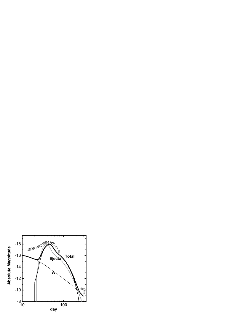
Figure 10.— Fallback model light curves. Shown here are the fall back model with $t_{\rm acc}=40^{\rm d}$, $\dot{M}_{\rm ej}=1.2\times 10^{-2}M_{\odot}{\rm d}^{-1}$ (black thin solid), and $t_{\rm acc}=20^{\rm d}$, $\dot{M}_{\rm ej}=2.0\times 10^{-2}M_{\odot}{\rm d}^{-1}$ (gray thin solid). The contribution from the blob (Model A) is also shown (dashed). The sum of the ejecta contribution (for the model with $t_{\rm acc}=40^{\rm d}$) and the blob contribution is shown by the thick curve. See Appendix A for details.

In the following scenarios (§5.3 and §5.4), it is interpreted that the low mass blob dominates the optical light in the first peak and the late phase (§4.2). We examine whether the second peak can be reproduced by any scenarios without producing too strong emission in the late phase. If this condition is satisfied, the entire light curve could be explained by the combination of the second peak component plus the blob component.

We use the ejecta model of Tominaga et al. (2005) with $M_{\rm ej,peak}=7.3M_{\odot}$ and $E_{{\rm peak},51}=1.3$. As we have already replaced the ”high velocity” ⁵⁶Ni component of Tominaga et al. (2005) with the low mass blob (Model A or B; see §4.2), we set the mass fraction of ⁵⁶Ni at $v>1,600$ km s^-1 to be zero hereafter (the contribution of the blob is added to the synthetic light curve after the computation of this ejecta contribution).

One possible process that decreases $M$(⁵⁶Ni) with time is the fallback of the inner ⁵⁶Ni-rich region onto the central remnant (e.g., Woosley & Weaver 1995; Iwamoto et al. 2005). Figure 10 shows the examples of synthetic light curves of supernovae hypothetically undergoing fallback (see Appendix A for details).

The model assumes that the accretion begins at a specific time ($t_{\rm acc}$), and that the mass accretion rate after the time $t_{\rm acc}$ obeys the form $\dot{M}_{\rm ej}\propto t^{-5/3}$. These are qualitatively expected in spherically symmetric fallback (e.g., Woosley & Weaver 1995; Iwamoto et al. 2005). The light curve of SN 2005bf can be reproduced in this context only if we assume $t_{\rm acc}\mathrel{\hbox to0.0pt{\lower 4.0pt\hbox{\hskip 1.0pt$\sim$}\hss}\raise 1.0pt\hbox{$>$}}20^{\rm d}$.

Difficulties encountered in the spherical fallback scenario are the following (Fig. 11; see Appendix B for details):

• $E_{{\rm peak},51}\sim 1-1.5$ is too large to cause the spherical hydrodynamic fallback.

• Fallback should take place very late, later than 10 days since the explosion. The time scale of the spherical fallback in the He star progenitor model is much shorter than 10 days (Figure 11).

The problem in the energy may be relaxed by considering an asymmetric explosion, because the velocity in the weak-explosion direction may be sufficiently small compared with escape velocity. The problem in the time scale may be overcome by introducing some mechanism to delay the fallback, e.g., by disk accretion (e.g., Mineshige, Nomoto, & Shigeyama 1993). However, it seems difficult to realize the condition that the ⁵⁶Ni-rich region experiences the fallback in a period of $\sim 1$ month (e.g., Figures 2 – 4 of Mineshige et al. 1997).

Figure 11.— The fallback mass as a function of time as obtained by a set of hydrodynamic simulations with varying explosion energy for a $7.3M_{\odot}$ He star model (black curves; the values of the final kinetic energy are shown in the figure). Also shown are those used to reproduce the light curve (Fig. 10) with two different fallback time scale (gray curves). See Appendix B for details.

5.4. Central Remnant’s Activity?

Another possibility is a different type of the energy source for the second peak. Other than ⁵⁶Ni and ⁵⁶Co, a possible heating source is the interaction between the ejecta and CSM. However, there is a strong argument against its responsibility for energizing the light curve of SN 2005bf. The light curve shows a slow rise to the peak ($t\sim 40^{\rm d}$), which is typical characteristics of diffusion of photons from deep in the ejecta. Also, there is no indication of strong interaction in its spectra around the peak.

The heating source should be buried deep in the ejecta, and it should be capable of producing the total energy input $\mathrel{\hbox to0.0pt{\lower 4.0pt\hbox{\hskip 1.0pt$\sim$}\hss}\raise 1.0pt\hbox{$>$}}10^{49}$ erg, at the maximum rate of $\mathrel{\hbox to0.0pt{\lower 4.0pt\hbox{\hskip 1.0pt$\sim$}\hss}\raise 1.0pt\hbox{$>$}}10^{43}$ erg s^-1. Except radioactivity, a possible source that satisfies these conditions could be the activity of the central compact remnant. Indeed, the peculiar features in the early phases led Tominaga et al. (2005) to speculate the formation of a strongly magnetized neutron star (a magnetar). Folatelli et al. (2006) speculated that SN 2005bf would be driven by the central engine similar to that in gamma-ray bursts, for which a popular idea is a black hole and an accretion disk system (Woosley 1993).

Since the luminosity emitted from a system consisting of a black hole and an accretion disk is expected not to exceed $\sim 10^{43}$ erg s^-1 because of neutrino losses (e.g., Janiuk et al. 2004), we consider a potentially more effective mechanism of emitting photons, i.e., a magnetar. The energy input is assumed to take the following form as a function of the position in the ejecta ($v$, expressed in velocity space) and time ($t$):

$$L_{\gamma}(v,t)=L_{0}\left(1.0+2.0\times\frac{t}{t_{0}}\right)^{-\beta}d(v)\ ,$$ (7)

where $d(v)=D\exp(-v/v_{0})$ if $v\leq 3000$ km s^-1 and $d(v)=0$ if $v>3000{\rm kms}^{-1}$, with $D$ the normalized constant. Here $L_{0}$ is the initial energy injection rate in the form of high energy photons, $t_{0}$ is characteristic time scale, and $v_{0}$ is characteristic length scale, and $\beta$ is the decay temporal index.

We assume the photon index of $-2.5$, as is similar to that of the Crab Pulsar (e.g., Davidson & Fesen 1985). We also assume that the minimum energy of the photon is 1 keV for the input high energy spectrum. Since the optical depth to these high energy photons is very large at the epochs considered here, details of the spectral index and the cut-off energy do not affect the result sensitively (see also Kumagai et al. 1991).

The density distribution of the ejecta model is taken from Tominaga et al. (2005) with the reconstruction of $M_{\rm ej}$ and $E_{51}$ in a self-similar manner. We set ⁵⁶Ni mass fraction zero throughout the ejecta to investigate the contribution of this hypothetical energy source. In the model shown in Figure 12, we used $M_{\rm ej}=8.0M_{\odot}$, $E_{51}=1.3$, which is within the range to explain the early phase spectra (Tominaga et al. 2005).

With the energy input and the ejecta model, the high energy radiation transport is solved by the Monte Carlo code described in Maeda (2006c). The optical photon transport is solved by the method described in §4 (see also Maeda et al. 2006b). Figure 12 shows the model with the following parameters:

• $L_{0}=8\times 10^{43}$ erg s^-1,

• $t_{0}=60^{\rm d}$,

• $v_{0}=2,500$ km s^-1, and

• $\beta=4$.

The position of the second peak is roughly reproduced irrespective of the input parameters, since the diffusion time scale mainly determines the peak date. The large peak luminosity and the rapid decline after the second peak can qualitatively be explained if $L_{0}\mathrel{\hbox to0.0pt{\lower 4.0pt\hbox{\hskip 1.0pt$\sim$}\hss}\raise 1.0pt\hbox{$>$}}10^{44}$ erg s^-1 and $t_{0}\mathrel{\hbox to0.0pt{\lower 4.0pt\hbox{\hskip 1.0pt$\sim$}\hss}\raise 1.0pt\hbox{$<$}}60^{\rm d}$. Large $L_{0}$ is expected if the central remnant is a strongly magnetized neutron star. The relations between the model parameters and physical quantities are discussed in §6.

Figure 12.— Synthetic light curve with the putative energy input from the central remnant (thick solid). The model parameters are as follows: $L_{0}=8\times 10^{43}$ erg s^-1, $t_{0}=60^{\rm d}$, $\beta=4$. The input luminosity of the remnant (thick dashed) and the contribution from the blob (thin dashed) are also shown. See §5.4 for details.

6. The HYPOTHESIS – A BIRTH EVENT OF A MAGNETAR

In §5, we have shown that the light curve of SN 2005bf is explained by the energy input from a magnetar left behind the explosion. In this section, we relate the model parameters to physical quantities, and discuss consequences and implications of the scenario.

• $L_{0}\mathrel{\hbox to0.0pt{\lower 4.0pt\hbox{\hskip 1.0pt$\sim$}\hss}\raise 1.0pt\hbox{$>$}}10^{44}$ erg s^-1 and $t_{0}\mathrel{\hbox to0.0pt{\lower 4.0pt\hbox{\hskip 1.0pt$\sim$}\hss}\raise 1.0pt\hbox{$<$}}60^{\rm d}$ is required to reproduce the large peak luminosity and the rapid decline after the second peak. If interpreted as a pulsar energy input, these two conditions are satisfied only if the remnant is a millisecond magnetar (i.e., the surface magnetic field is $B_{\rm mag}\sim 10^{14-15}$ gauss, and the initial spin period $P_{0}\sim 5-10$ ms).

  The model parameters, $L_{0}=8\times 10^{43}$ erg s^-1 and $t_{0}=60^{\rm d}$, corresponds to a pulsar with the magnetic field $B_{\rm mag}\sim 3\times 10^{14}(P_{0}/10\ {\rm ms})^{2}\sqrt{0.1/f_{\rm rad}}$ gauss, using the dipole radiation formula (Ostriker & Gunn 1969; see also Rees & Meszaros 2000). Here $P_{0}$ is the initial spin period and $f_{\rm rad}$ is a fraction of energy going into the radiation. The total energy injection with these parameters is $\sim 7\times 10^{50}(f_{\rm rad}/0.1)^{-1}$ erg, a fraction of which might be consumed to increase the kinetic energy of the SN ejecta to $E_{51}=1-1.5$ and/or to develop the pulsar nebula in the early phase (see below).

• The relatively large breaking index $\beta=4$ is required to reproduce the large contrast between the peak and the tail, but it is still within the range of the decay rates inferred for galactic pulsars.

  The temporal index $\beta=2$ is expected for the energy input from a pulsar slowed down predominantly by the magnetic dipole radiation. It is also the case for similar models involving the conversion of the rotational energy to the energy of radiation or relativistic particles mediated purely by the magnetic field (e.g., Ostriker & Gunn 1969).

  If $\beta=4$, then the pulsar’s breaking index is $n=2$ ($\dot{\Omega}\propto\Omega^{n}$ by definition, where $\Omega$ is the rotational angular frequency), while the magnetic dipole model ($\beta=2$) predicts $n=3$. The breaking index as small as 2 is expected by dissipation processes mediated not only by the magnetic field (e.g., Menou, K., Perna, R., & Hernquist 2001), and is really inferred for most pulsars with the index measurement available (e.g., Livingstone, Kapsi, & Gavriil 2005 and references therein).

• Although the peak date can be reproduced irrespective of $v_{0}$ as the diffusion time scale mainly determines the peak date, a good fit to the light curve width around the peak is obtained if we set $v_{0}\sim 2,000-2,500$ km s^-1.

  This is larger than the average expansion velocity of the Crab pulsar wind nebula seen in X-rays (e.g., Mori et al. 2004): Assuming 2 kpc for the distance to the Crab nebula, the spatial extent of its X-ray image corresponds to the average expansion velocity of $\sim 500$ km s^-1. The early development and the relatively large size of the pulsar nebula in our light curve model might not be surprising, because of small $t_{0}$ and large $L_{0}$. Injection of a fraction of the total energy [$\sim 7\times 10^{50}(f_{\rm rad}/0.1)^{-1}$ erg: see above] into the nebula within $\sim t_{0}$ would naturally explain large $v_{0}$.

• A connection to other SNe Ib/c is interesting. A typical pulsar with $B_{\rm mag}\sim 10^{12}$ gauss and $P_{0}\sim 30$ ms produces only negligible contribution to the light curve compared to the ⁵⁶Ni/Co energy input during the first few years. In the pulsar energy input scenario, large $L_{0}$ and small $t_{0}$ (thus large $B_{\rm mag}$ and small $P_{0}$) are required to make the light curve doubly peaked as seen in SN 2005bf. Such that, the model is consistent with singly peaked light curves of other SNe Ib/c, which are believed to leave a typical neutron star (except probably the Gamma-Ray Burst related SNe).

  Another interesting implication is related to SN 2006aj associated with an X-Ray Flash (XRF) 060218 (Pian et al. 2006). SN2006aj/XRF060218 is suggested to be driven by a neutron star formation, presumably a magnetar, through observations at early phases (Mazzali et al. 2006) and at late phases (Maeda et al. 2007). SN 2006aj showed a singly-peaked light curve as is similar to other SNe Ib/c explained by usual ⁵⁶Ni heating scenario. This behavior is explained, if the newly born neutron star in SN 2006aj has even larger $B_{\rm mag}$ and/or smaller $P_{0}$ than in SN 2005bf. In this case, the characteristic time scale ($t_{0}$) of the high energy input becomes as small as $t_{0}\mathrel{\hbox to0.0pt{\lower 4.0pt\hbox{\hskip 1.0pt$\sim$}\hss}\raise 1.0pt\hbox{$<$}}10^{\rm d}$ since the dipole radiation is scaled as $L_{0}\propto B_{\rm mag}^{2}P_{0}^{-4}$. A magnetar may also spin down much shorter than $t\sim 1^{\rm d}$ without emitting electromagnetically, if it blows a massive wind (Thompson, Chang, & Quataert 2004). Most of the emission is then consumed by adiabatic lose because of high density in such an early epoch. Such that, the contribution of the pulsar energy input to the light curve is negligible in this case, and a part of the pulsar energy input is transferred to the SN ejecta. This may explain $E_{51}\sim 2$ in SN 2006aj.

  Thus, we suggest that SN 2005bf is an event linking usual SNe Ib/c and SN 2006aj/XRF 060218. In our proposed scenario, these are connected by the formation of a neutron star with different $B_{\rm mag}$ and $P_{0}$.

Although the choice of the model parameters look reasonable, there is a caveat. Since the nature of young pulsar is still in active debate, more detailed study of the magnetar hypothesis is necessary. For example, even the very basic assumption in this model, i.e., whether the pulsar wind nebula is formed within a few days since the explosion, is still under debate (e.g., Fryer, Colgate, & Pinto 1999).

7. CONCLUSIONS

7.1. Blob Model for the First Peak and the Nebular Epoch

In this paper, we have presented the results from spectroscopic and photometric observations of SN 2005bf at $t\sim 300^{\rm d}$. Our theoretical considerations are summarized as follows.

• The faint nebular emission, composed of blueshifted emission lines ([OI], [CaII], [FeII]), can be understood if the emission in the late phases is dominated by a low mass blob with $M_{\rm ej,neb}\sim 0.1-0.4M_{\odot}$, $M$(⁵⁶Ni)_neb $\sim 0.02-0.06M_{\odot}$.

• The blueshift is reproduced either by a unipolar blob with the center-of-mass velocity $v\mathrel{\hbox to0.0pt{\lower 4.0pt\hbox{\hskip 1.0pt$\sim$}\hss}\raise 1.0pt\hbox{$>$}}2,000-5,000$ km s^-1, or by self-absorption of the optical light as seen in SNe 1990I and 1987A.

• The emission line profiles from different elements suggest that the blob in itself has layered structure.

• The optical luminosities at the first peak ($t\sim 20^{\rm d}$) and at the nebular phases ($t\sim 300^{\rm d}$) are consistent with the emission from this blob.

• The line ratios suggest the abundance pattern similar to what is expected from progenitor stars with $M_{\rm ms}\sim 20-25M_{\odot}$, as is consistent with the lower end of the estimate given by the previous works (Tominaga et al. 2005).

It should be mentioned that recently a new paradigm is entering into the scene of core-collapse physics, either standing accretion shock instability or g-mode oscillation of the newly born neutron star. Some models do predict unipolar supernova explosions (Burrows et al. 2006). SN 2005bf could be the first extreme example of this kind of explosions.

7.2. Energy Source for the Second Peak

At the nebular phases, SN 2005bf turns out to be extremely faint ($R=24.4$ mag at $t\sim 273^{\rm d}$). It is dominated by the contribution from the low-mass blob. The bulk of the emission expected from $M$(⁵⁶Ni)_peak $\sim 0.3M_{\odot}$, as is derived from the second peak luminosity at $t\sim 40^{\rm d}$, is missing. Where is the missing emission is a question we tried to answer in this paper.

As the energy source should be buried deep in the ejecta, the peak date is determined by the diffusion time scale. Therefore, the ejecta mass and the energy derived by the previous works should give a good estimate even if the energy source responsible to the peak luminosity is different. In conclusion, the main sequence mass is $M_{\rm ms}\sim 20-25M_{\odot}$,

Four possibilities are examined in §5: (1) accelerated gamma-ray and positron escape, (2) almost $100\%$ shielding of the optical light, (3) fallback of ⁵⁶Ni-rich materials, and (4) possible central object’s activity. Among these, the first three possibilities have difficulties.

(1) No physically reasonable mechanism is found to reduce the gamma-ray and positron opacity (§5.1). (2) The extreme self-absorption scenario looks to be inconsistent with the detail of the observations (§5.2). (3) The fallback scenario is found to be difficult to work, unless some additional mechanisms (e.g., delayed fallback by disk accretion) could rescue the situation (§5.3).

One can still consider a combination of some of them. For example, assume that gamma-rays but not positrons can escape effectively and that the optical output is reduced by a factor of 10 – 15 by self–absorption. This is more extreme than in Model B and other dust-forming SNe, but less than examined in §5.2. Then the late-time luminosity could be reproduced (see the light curve with small $\kappa_{\gamma}$ in Figure 8). A question here is if these phenomena, each of which is unusual, can by chance take place together.

7.3. Magnetar Hypothesis

The last possibility, the central remnant activity, yields a reasonable fit to the light curve if the central remnant is a magnetar with $B_{\rm mag}\sim 10^{14-15}$ gauss and $P_{0}\sim 10$ ms. The scenario has advantages compared to other models as summarized in the following.

• The magnetar hypothesis can explain two peculiar features in the light curve in the same context. The rapid declining at $t\sim 60^{\rm d}$ and the faintness at $t\sim 300^{\rm d}$ are essentially difficult in the standard ⁵⁶Ni/Co heating scenario. These two could be explained by combination of two (very) peculiar natures, such as the reduced $\gamma$-ray opacity for the former and the huge dust extinction for the latter, but in the magnetar hypothesis these are attributed to the single physical reason.

• The blueshift of the nebular emission lines could be related to the pulsar kick. The blueshift can be interpreted as ejection of the unipolar blob with $v\mathrel{\hbox to0.0pt{\lower 4.0pt\hbox{\hskip 1.0pt$\sim$}\hss}\raise 1.0pt\hbox{$<$}}2,000$ km s^-1 (Model A). With $M_{\rm neb}\sim 0.1M_{\odot}$ in the blob, the newly formed neutron star with $\sim 1.4M_{\odot}$ would have the kick velocity of $v_{\rm kick}\mathrel{\hbox to0.0pt{\lower 4.0pt\hbox{\hskip 1.0pt$\sim$}\hss}\raise 1.0pt\hbox{$>$}}140$ km s^-1.

• The scenario is compatible to relatively large $E_{51}\sim 1-1.5$, as the magnetar activity could also increase the ejecta kinetic energy. It could also be compatible to the estimated mass, $M_{\rm ms}\sim 20-25M_{\odot}$, which is close to the upper limit for the neutron star formation.

• The rarity of SN 2005bf-like supernova is consistent with the rarity of a magnetar, although there are observational biases in the search of neutron stars.

Summarizing, we suggest that SN 2005bf is driven by a strongly magnetized neutron star (a magnetar), being the birth place of a soft gamma-ray repeater or an anomalous X-Ray pulsar. In our scenario, SN 2005bf is an event which links usual SNe Ib/c and SN 2006aj/XRF 060218: As the magnetic activity and/or the spin frequency increases, the resulting SN becomes usual SNe Ib/c (a typical neutron star, whose contribution to the light curve is negligible), SN 2005bf-like supernova (for which the magnetar makes the doubly-peaked light curve), and finally SN 2006aj/XRF 060218-like high energy transient (again the light curve becomes singly peaked, since the magnetar activity is consumed to produce the high energy transient and to increase the ejecta kinetic energy).

Appendix A Light Curves of Supernovae with Fallback

The light curves of supernovae undergoing fallback (Fig. 10) are computed as follows. They are computed using the same code described in §4. The same ejecta model with $M_{\rm ej,peak}=7.3M_{\odot}$ and $E_{{\rm peak},51}=1.3$ is adopted, except for the ⁵⁶Ni distribution. Here we set the ⁵⁶Ni mass fraction above $1,600$ km s^-1 zero since we are not concerned with the first peak (see §5.3).

We remove the ejecta materials (including ⁵⁶Ni) from the innermost region as a function of time. $M_{\rm ej}$ is decreased according to

$$\dot{M}_{\rm ej}(t)=\dot{M}_{\rm ej}(t_{\rm acc})\times\left(\frac{t}{t_{\rm acc}}\right)^{-\frac{5}{3}}\ ,$$ (A1)

where $t_{\rm acc}$ is the date when the fallback is assumed to begin. Thus, $M_{\rm ej}(t)=M_{\rm ej,peak}$ for $t\leq t_{\rm acc}$. This temporal dependence is expected in the limit of negligible pressure support and confirmed by numerical calculations (Woosley & Weaver 1995; also see Appendix B). The model parameters are as follows:

• $t_{\rm acc}=40^{\rm d}$ and $\dot{M}_{\rm ej}(t_{\rm acc})=1.2\times 10^{-2}M_{\odot}$ d^-1, and

• $t_{\rm acc}=20^{\rm d}$ and $\dot{M}_{\rm ej}(t_{\rm acc})=2.0\times 10^{-2}M_{\odot}$ d^-1.

The corresponding histories of the mass accretion are shown in Figure 11.

Appendix B Spherical Fallback

Figure 11 for the histories of the fallback mass accretion rate is computed as follows. A set of 1D explosion simulations are performed for a $7.3M_{\odot}$ He core of a star with $M_{\rm ms}=25M_{\odot}$, using a 1D PPM (piecewise parabolic method) hydrodynamic code. We have varied the explosion energy which is injected at $M_{r}=1.8M_{\odot}$ and investigated the relation among the final kinetic energy ($E$), the amount of the fallback materials ($M_{\rm acc}$), and the timescale of the fallback ($t_{\rm acc}$). Figure 11 shows the histories of the fallback obtained in the simulations. Also shown in Figure 11 are the histories of the fallback assumed to compute the light curves in Figure 10. By comparing the shapes of the curves in Figure 11, it is seen that the fallback temporal dependence used in the light curve computations ($\dot{M}_{\rm ej}\propto t^{-5/3}$) is a good approximation for the spherical hydrodynamic fallback.

From these simulations, we find the following relation. Smaller $E$ results in larger $M_{\rm acc}$ and smaller $t_{\rm acc}$. The light curve fitting requires $t_{\rm acc}$ much larger than that obtained by the hydrodynamic simulations. Also, $E_{{\rm peak},51}=1-1.5$ (Table 1) is too large to make the fallback effectively work.

We set the position of the energy injection at $M_{r}=1.8M_{\odot}$ in this examination. If we take larger $M_{r}$ for the injection, then the binding energy in the surrounding layers is smaller. Then it acts like a less massive star as long as the fallback is concerned. A less massive star experiences the fallback for smaller $E$ (see Iwamoto et al. 2005). According to our simulations, the final kinetic energy dividing the fallback and no-fallback is $E_{51}\sim 0.2$ for $M_{r}=3.6M_{\odot}$, which is smaller than $E_{51}\sim 0.7$ for $M_{r}=1.8M_{\odot}$. For $M_{r}=3.6M_{\odot}$, $t_{\rm acc}$ can be a bit longer than for $M_{r}=1.8M_{\odot}$, but still $t_{\rm acc}\mathrel{\hbox to0.0pt{\lower 4.0pt\hbox{\hskip 1.0pt$\sim$}\hss}\raise 1.0pt\hbox{$<$}}10^{\rm d}$. Because $E_{{\rm peak},51}\sim 1-1.5$, the larger $M_{r}$ makes the fallback scenario less likely to be realized. In sum, changing $M_{r}$ does not solve the problem.

References

- (1) Anupama, G.C., et al. 2005, ApJ, 631, L125
- (2) Bowyer, C.S., & Field, G.B. 1969, Nature, 223, 573
- (3) Burrows, A., Livne, E., Dessart, L., Ott, C.D., & Murphy, J. 2006, ApJ, 640, 878
- (4) Cappellaro, E., Mazzali, P.A., Benetti, S., Danziger, I.J., Turatto, M., Della Valle, M., & Patat, F. 1997, A&A, 328, 203
- (5) Davidson, K., & Fesen, R.A. 1985, ARAA, 23, 119
- (6) Elmhamdi, A., Danziger, I.J., Cappellaro, E., Della Valle, M., Gouiffes, C., Phillips, M.M., & Turatto, M. 2004, A&A, 426, 963
- (7) Filippenko, A.V. 1991, IAU Circ. 5169
- (8) Folatelli, G., et al. 2006, ApJ, 641, 1039
- (9) Fransson, C., & Chevalier, R. 1987, ApJ, 322, L15
- (10) Fransson, C., & Chevalier, R. 1989, ApJ, 343, 323
- (11) Fryer, C.L., Clogate, S.A., & Pinto, P.A. 1999, ApJ, 511, 885
- (12) Hatano, K., Branch, D., Nomoto, K., Deng, J., Maeda, K., Nugent, P., & Aldering, G. 2001, BAAS, 198, 3902
- (13) Houck, J.C., & Fransson, C. 1996, ApJ, 456, 811
- (14) Hungerford, A., Fryer, C.L., Rockefeller, G. 2005, ApJ, 635, 487
- (15) Iwamoto, N., Umeda, H., Tominaga, N., Nomoto, K., & Maeda, K. 2005, Science, 309, 451
- (16) Janiuk, A., Perna, R., Matteo, T. Di., & Czerny, B. 2004, MNRAS, 355, 950
- (17) Kashikawa, N., et al. 2002, PASJ, 54, 819
- (18) Kumagai, S., Shigeyama, T., Hashimoto, M., & Nomoto, K. 1991, A&A, 243, L13
- (19) Landolt, A. U. 1992, AJ, 104, 340
- (20) Livingstone, M.A., Kapsi, V.M., & Gavriil,F.P. 2005, ApJ, 633, 1095
- (21) Maeda, K., Nakamura, T., Nomoto, K., Mazzali, P.A., Patat, F., & Hachisu, I. 2002, ApJ, 565, 405
- (22) Maeda, K., Mazzali, P.A., Deng, J., Nomoto, K., Yoshii, Y., Tomita, H., & Kobayashi, Y. 2003, ApJ, 593, 931
- (23) Maeda, K., Nomoto, K., Mazzali, P.A., & Deng, J. 2006a, ApJ, 640, 854
- (24) Maeda, K., Mazzali, P.A., & Nomoto, K. 2006b, ApJ, 645, 1331
- (25) Maeda, K. 2006c, ApJ, 644, 385
- (26) Maeda, K., et al. 2007, ApJ, 658, L5
- (27) Massey, P., Strobel, K., Barnes, J. V., & Anderson, E. 1988, 328, 315
- (28) Massey, P., & Gronwall, C. 1990, ApJ, 358, 344
- (29) Matheson, T., Filippenko, A.V., Li, W., & Leonard, D.C. 2001, ApJ, 121, 1648
- (30) Mazzali, P.A., Nomoto, K., Patat, F., & Maeda, K. 2001, ApJ, 559, 1047
- (31) Mazzali, P.A., Deng, J., Maeda, K., Nomoto, K., Filippenko, A.V., & Matheson, T. 2004, ApJ, 614, 858
- (32) Mazzali, P.A., et al. 2005, Science, 308, 1284
- (33) Mazzali, P.A., et al. 2006, Nature, 442, 1018
- (34) Menou, K., Perna, R., & Hernquist, L. 2001, ApJ, 554, L63
- (35) Milne, P.A., The, L.-S., & Leising, M.D. 2001, ApJ, 559, 1019
- (36) Mineshige, S., Nomoto, K., & Shigeyama, T. 1993, A&A, 267, 95
- (37) Mineshige, S., Nomura, H., Hirose, M., Nomoto, K., & Suzuki, T. 1997, ApJ, 489, 227
- (38) Modjaz, M., Kirshner, R., & Challis, P. 2005, IAU Circ., 8522, 2
- (39) Monard, L.A.G. 2005, IAU Circ., 8507, 1
- (40) Moore, M., & Li, W. 2005, IAU Circ., 8507, 1
- (41) Mori, K., Burrows, D.N., Hester, J.J., Pavlov, G.G., Shibata, S., & Tsunemi, H. 2004, ApJ, 609, 186
- (42) Motohara, K., et al. 2006, ApJ, 652, L101
- (43) Nagase, F., Hayakawa, S., Sato, N., Masai, K., & Inoue, H. 1986, PASJ, 38, 547
- (44) Nakamura, T., Mazzali, P.A., Nomoto, K., & Iwamoto, K. 2001a, ApJ, 550, 991
- (45) Nakamura, T., Umeda, H. Iwamoto, K., Nomoto, K., Hashimoto, M., Hix, W.R., & Thielemann, F.-K. 2001b, ApJ, 555, 880
- (46) Nomoto, K., Tominaga, N., Umeda, H., Kobayashi, C., & Maeda, K. 2006, Nuc. Phys. A., 777, 424 (astro-ph/0605725)
- (47) Nozawa, T., Kozasa, T., Umeda, H., Maeda, K., & Nomoto, K. 2003, ApJ, 598, 785
- (48) Ostriker, J.P., & Gunn, J.E. 1969, ApJ, 157, 1395
- (49) Patat, F., et al. 2001, ApJ, 555, 900
- (50) Pian, E., et al. 2006, Nature, 442, 1011
- (51) Rees, M.J., & Meszaros, P. 2000, ApJ, 545, L73
- (52) Richardson, D., Branch, D., & Baron, E. 2006, AJ, 131, 2233
- (53) Ruiz-Lapuente, P., & Lucy, L.B. 1992, ApJ, 400, 127
- (54) Soderberg, A.M., Berger, E., Ofek, E., & Leonard, D.C. 2005, The Astronomer’s Telegram, 646
- (55) Thompson, T.A., Chang, P., & Quataert, E., 2004, ApJ, 611, 380
- (56) Tominaga, N., et al. 2005, ApJ, 633, L97
- (57) Tomita, H., et al. 2006, ApJ, 644, 400
- (58) Wang, L., & Baade, D. 2005, IAU Circ., 8521, 2
- (59) Woosley, S.E., 1993, ApJ, 405, 273
- (60) Woosley, S.E., & Weaver, T.A. 1995, ApJS, 101, 181