A deeper X-ray study of the core of the Perseus galaxy cluster: the power of sound waves and the distribution of metals and cosmic rays

Abstract

We make a further study of the very deep Chandra observation of the X-ray brightest galaxy cluster, A 426 in Perseus. We examine the radial distribution of energy flux inferred by the quasi-concentric ripples in surface brightness, assuming they are due to sound waves, and show that it is a significant fraction of the energy lost by radiative cooling within the inner 75-100 kpc, where the cooling time is 4–5 Gyr, respectively. The wave flux decreases outward with radius, consistent with energy being dissipated. Some newly discovered large ripples beyond 100 kpc, and a possible intact bubble at 170 kpc radius, may indicate a larger level of activity by the nucleus a few 100 Myr ago. The distribution of metals in the intracluster gas peaks at a radius of about 40 kpc and is significantly clumpy on scales of 5 kpc. The temperature distribution of the soft X-ray filaments and the hard X-ray emission component found within the inner 50 kpc are analysed in detail. The pressure due to the nonthermal electrons, responsible for a spectral component interpreted as inverse Compton emission, is high within 40 kpc of the centre and boosts the power in sound waves there; it drops steeply beyond 40 kpc. We find no thermal emission from the radio bubbles; in order for any thermal gas to have a filling factor within the bubbles exceeding 50 per cent, the temperature of that gas has to exceed 50 keV.

1 Introduction

The Perseus cluster, Abell 426, is the brightest galaxy cluster in the sky when viewed in the X-ray band. The cluster contains a bright radio source 3C 84 (Pedlar et al., 1990), the radio lobes of which are displacing the X-ray emitting thermal gas of the cluster (Böhringer et al., 1993; Fabian et al., 2000). The X-ray emission from the intracluster medium (ICM) is highly peaked in the centre and the radiative cooling time of the hot gas is less than 5 Gyr within a radius of 100 kpc, decreasing to $3\times 10^{8}\rm\thinspace yr$ within the central 10 kpc (Sanders et al., 2004). A cooling flow of several $100\hbox{$\hbox{$\rm\thinspace M_{\odot}$}\rm\thinspace yr^{-1}\,$}$ would take place if radiative energy losses from the inner ICM are not balanced by some form of energy injection. As expected from cooling, the gas temperature does drop from the outer value of 7 keV within the central 100 kpc but only down to about 2.5 keV with little X-ray emitting gas found at lower temperatures, except in coincidence with line-emitting filaments seen at optical wavelengths (Fabian et al., 2003a, 2006). Heating by the central radio source is widely considered responsible for balancing the radiative cooling, although the exact mechanisms by which the energy is transported and dissipated and a heating/cooling balance established have been unclear.

Similar behaviour is found in many X-ray peaked, cool-core clusters (see Peterson & Fabian 2006 for a review). The central galaxy in such clusters could grow considerably larger than observed if radiative cooling was unchecked. X-ray observations of their innermost regions provide an excellent means to study the feedback of an Active Galactic Nucleus (AGN) on its host galaxy in action. Here we use a long (900 ks) Chandra observations of the X-ray brightest cluster core to examine the energy balance and metallicity in considerable detail. The quality of the data, in terms of counts per arcsec, are much higher than available with any other cluster. We examine the power propagating through the core in terms of pressure ripples, or sound waves, and the cosmic-ray implications of a hard X-ray component. We also use the metallicity distribution, the temperature profile of the X-ray emitting gas across an optical filament and assess the thermal gas content of the radio bubbles.

No X-ray emission has been detected from within the radio bubbles (Schmidt et al., 2002; Sanders et al., 2004). Two depressions in the X-ray surface brightness are also found, to the north-west and south, not associated with high-frequency radio emission. These are likely to be ‘ghost’ radio bubbles which have detached from the nucleus and buoyantly risen in the gravitational field (Churazov et al., 2000; Fabian et al., 2000), an idea supported by weak low frequency radio spurs seen pointing towards their direction (Fabian et al., 2002b).

Surrounding the inner radio lobes are X-ray bright rims (Fabian et al., 2000) at a higher pressure than the outer regions, and separated from them by a weak isothermal shock (Fabian et al., 2006). Extending further into the clusters are concentric fluctuations in surface brightness. These are plausibly pressure and density ripples, in which case they are sound waves generated by the inflation of the radio bubbles (Fabian et al., 2003a, 2006). The period of the waves is about 10 Myr, close to the expected age of the bubbles due to buoyancy, and is not plausibly related to any other source of disturbance. Ripples due to sound waves have since been found in simulations (Ruszkowski et al., 2004; Sijacki & Springel, 2006). Such sound waves can transport significant energy in a roughly isotropic manner and so balance radiative cooling of the intracluster gas if they dissipate their energy over the surrounding 50–100 kpc (Fabian et al., 2003a; Ruszkowski et al., 2004; Fabian et al., 2005). Concentric ripple-like features are also found around M87 in the Virgo cluster, and are interpreted there as weak shocks (Forman et al., 2006). More powerful outbursts include those discovered in MS 0735.6+7421 (McNamara et al., 2005), Hercules A (Nulsen et al., 2005a) and Hydra A (Nulsen et al., 2005b).

Around the central galaxy in the Perseus cluster, NGC 1275, lies a giant line-emitting nebula (Lynds, 1970; Conselice et al., 2001), associated with cool $\sim 0.7$ keV X-ray emitting filaments (Fabian et al., 2003b) of $\sim 10^{9}\hbox{$\rm\thinspace M_{\odot}$}$ mass (Fabian et al., 2006). The H$\alpha$ emitting filaments appear to be have been drawn out of the central galaxy by the rising bubbles (Hatch et al., 2006).

There is spectral evidence for hard X-ray emission from the central region, found either with hot thermal (Sanders et al., 2004) or non-thermal (Sanders et al., 2005) models. The 2-10 keV luminosity of this emission is $\sim 5\times 10^{43}\hbox{$\rm\thinspace erg\rm\thinspace s^{-1}\,$}$.

The iron metallicity structure in the core of the cluster is inhomogeneous and complex (Schmidt et al., 2002; Sanders et al., 2004, 2005) with the abundance dropping in the very core. There are also structures such as high-metallicity ridge and blobs, which may be associated with the bubbles.

We use a Perseus cluster redshift of 0.0183 here, which gives an angular scale of 0.37 kpc per arcsec, assuming $H_{0}=70\hbox{$\hbox{$\rm\thinspace km\rm\thinspace s^{-1}\,$}\rm\thinspace Mpc^{-1}$}$.

2 Data preparation

The datasets analysed in this paper are those that were examined in Fabian et al. (2006). However here we used the standard ciao data preparation tools on the event files. We used the datasets from the Chandra archive which had gone through Reprocessing III (reprocessed using version 7.6.7.1 of the pipeline). Datasets 03209 and 04289 were not reprocessed at the time of the analysis, so we therefore went through each of the steps in the Science Threads to reprocess the data manually for these. The reprocessing was done prior to CALDB 3.3.0 (using gainfile acisD2000-01-29gain_ctiN0005.fits).

We filtered the level 2 event files for flares as in Fabian et al. (2006). We then reprojected each dataset to match the 04952 observation in sky coordinates. We also reprocessed a combined 980-ks blank sky observation file to use the same calibration files as used by the foreground observations. We randomised the order of the events in the background file in order to remove any potential spectral variability. The background file was split into sections, to provide a background for each foreground observation. The length of each section was chosen to have the same ratio to the total as the ratio of its respective foreground dataset to the total foreground. The exposure time of each section was adjusted to give the same count rate in the 9-12 keV band as its respective foreground (where there is no source). The background sections were then reprojected to the original level 2 event file for the matching observation, and then reprojected to the 04952 observation.

In addition we constructed separate background event files for each dataset to account for out-of-time events, where photons hit the detector while it is being read out. We used the make_readout_bg script (written by M. Markevitch) to construct these files from the original level 1 event files after filtering bad time periods. The readout backgrounds were reprojected to match the 04952 observation.

For the spectral analysis, for a particular region we extracted foreground spectra from each of the foreground event files relevant for the region in question. Similarly we made spectra from the background event files and and readout background files. The foreground spectra were added together to make a total foreground spectrum with a total exposure time. Background spectra were added similarly to make a total background, and so were readout background spectra.

We also created responses and ancillary responses for each of the foreground datasets, weighting the responses according to the number of counts in each spatial region between 0.5 and 7 keV. A response and ancillary response was made for the total foreground spectrum by adding the responses and ancillary responses for the individual observations, weighting according to the number of counts between 0.5 and 7 keV.

To analyse the spectra, we fit them in xspec version 11.3.2 (Arnaud, 1996). The energy range 0.6 to 8 keV was used during fitting, and the spectra were grouped to have at least 20 counts per spectral bin. The spectra extracted from the appropriate region from the background files was used as a background spectrum, and the spectra from the region from the readout background files was used as a ‘correction file’.

In this paper we use the apec (Smith et al., 2001) and mekal (Mewe et al., 1985; Mewe et al., 1986; Kaastra, 1992; Liedahl et al., 1995) thermal spectral models. To model photoelectric absorption we use the phabs model (Balucinska-Church & McCammon, 1992).

3 X-ray surface brightness

3.1 Surface brightness images

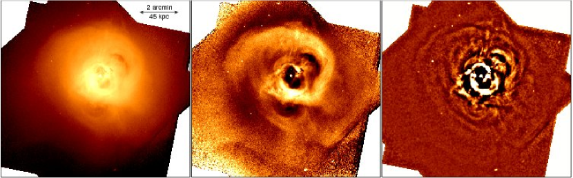
Figure 1: Surface brightness images of the cluster. (Left) 0.3 to 7 keV full band X-ray exposure-map-corrected image, smoothed with a Gaussian of 1.5 arcsec. (Centre) Image after subtracting King model fits to 40 sectors, smoothed with a Gaussian of 1.75 arcsec. (Right) Original image after high-pass filtering, then smoothing with a Gaussian of 1.5 arcsec.

Fabian et al. (2003a) and Fabian et al. (2006) used unsharp-masking techniques to reveal the surface brightness fluctuations in the intracluster medium. Unsharp masking increases the noise in the outer parts of the image where there are relatively few counts. We have experimented with several techniques to improve on simple unsharp masking. We split the exposure-map-corrected image (Fig. 1 left panel) into 40 sectors (centred on the central nucleus), and fitted a King model to each of the sectors outside of a radius of 13 arcsec (to avoid the central source). We constructed a model surface brightness image by iterating over each pixel, using the value obtained by interpolating in angle between the model surface brightness profiles of the two neighbouring sectors. This model image was then subtracted from the original image, resulting in Fig. 1 (centre panel). The image very clearly highlights the surface brightness increase associated with the low-temperature spiral in the cluster (Fabian et al., 2000; Churazov et al., 2000). A number of other features can be seen, including the possible cold front to the south, the ‘bay’ and the ‘arc’ (figure 2 in Fabian et al. 2006). It does not show the ripples particularly clearly (except perhaps by the southern bubble) as the cool swirl is dominant.

The ripples are more clearly highlighted using a Fourier high-pass filter technique. A two-dimensional fast Fourier transform of the exposure-map-corrected image was made. We removed the low frequency components with a wavelength greater than 75 arcsec. Frequency components between wavelengths of 75 and 38 arcsec were allowed through using with a linear filter increasing from 0 to 1 between these wavelengths. All shorter wavelengths were left to remain. The Fourier-transformed image was then transformed back to give Fig. 1 (right panel) after light smoothing. This technique removes the cool swirl and the underlying cluster emission. It clearly reveals the ripples, presumably sound waves generated by the inflation of the bubbles, discovered by Fabian et al. (2003a). It shows a previously unseen ripple near the edge of the image to the east.

3.2 Sector across eastern ripples

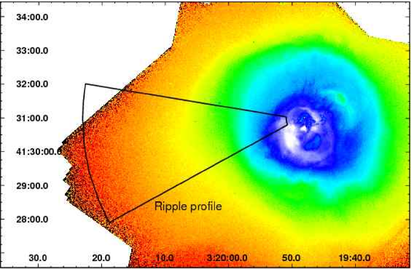
Figure 2: Full band X-ray image showing the sector examined for surface brightness fluctuations (Fig. 3). The region is centred on the inner NE radio bubble to better match the surface brightness contours.

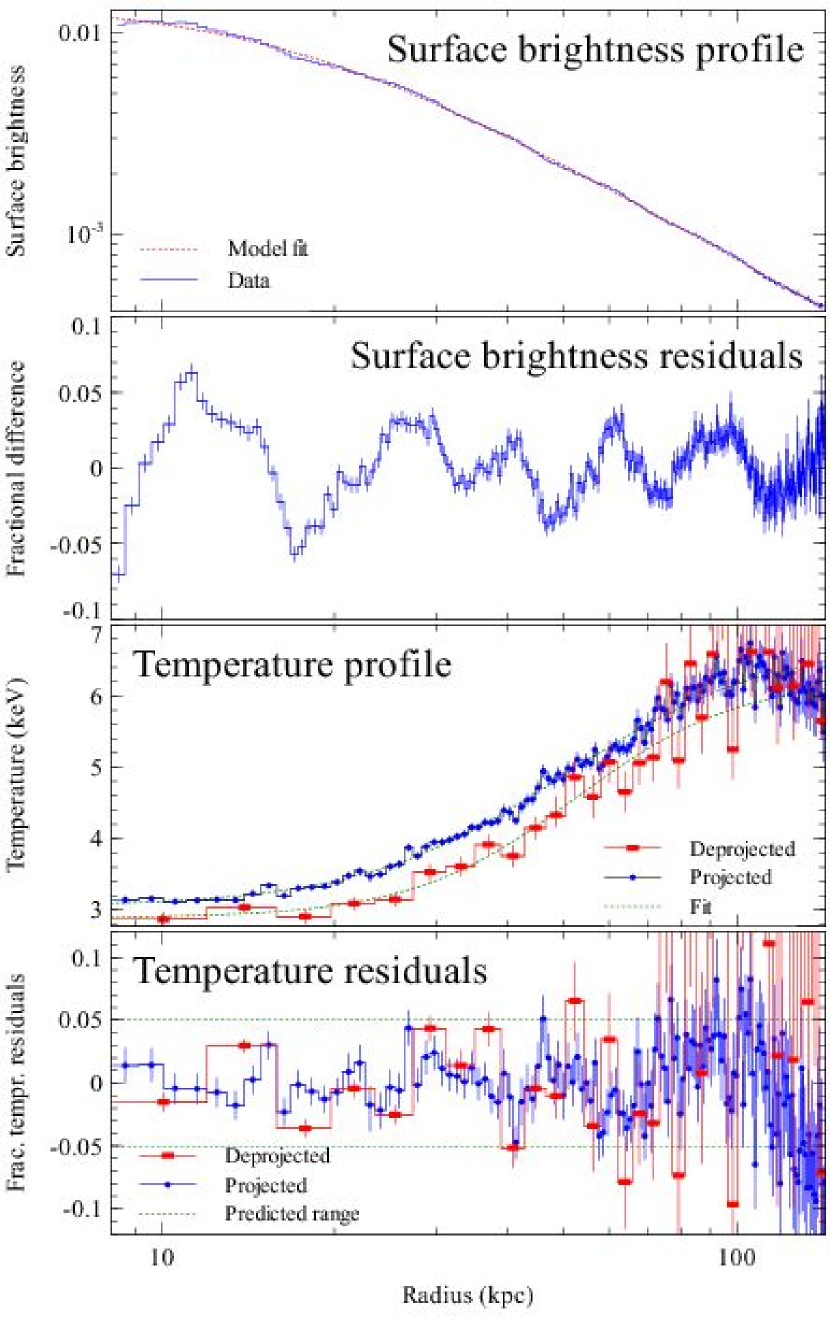
Figure 3: Surface brightness profile to the ESE of the cluster core (0.3 to 7 keV), also showing a King model fit, fractional residuals from the fit, a temperature profile with fit, and fractional residuals from the temperature fit. The dotted lines on the temperature residual plot show the expected variation associated with a 3 per cent surface brightness fluctuation. Note that the profile is not centred on the nucleus.

To quantitatively examine the ripples, we have examined the surface brightness in a sector shown in Fig. 2. We show in Fig. 3 (top panel) a surface brightness profile (in the 0.3 to 7 keV band) made to the east-south-east (ESE) of the cluster core. Also shown in the top panel is a King model fit to the profile. In the second panel we show the fractional residuals to the fit, clearly showing the oscillations in surface brightness observed in Fig. 1 (right panel) at the few percent level (the first peak in this figure corresponds to the bright rim of the radio bubbles).

To look for any temperature structure associated with the oscillations we fitted phabs absorbed apec thermal spectral models to spectra extracted in annuli from the spectra. The fitting procedure allowed the temperature, metallicity, normalisation and absorption to vary, and minimised the C-statistic (Cash, 1979) in each fit. The projected temperature profile is shown in the third panel of Fig. 3. We also show the results from fitting the same model (using the $\chi^{2}$ statistic) to deprojected spectra in larger bins. We used the deprojection method in Appendix A to create the deprojected spectra.

We finally show the residuals from a simple ‘$\eta$ model’ (Allen et al., 2001) fits to the projected and deprojected temperature profiles (Fig. 3 fourth panel) superficially. There is no obvious temperature structure associated with the ripples in this location of the cluster. The amount of temperature variation expected from the surface brightness fluctuations can be estimated. Simulations of thermal spectra in xspec shows that the surface brightness is independent of temperature at constant density in the temperature range 3–6 keV. If the adiabatic index of the ICM is $\gamma=5/3$, assuming the ideal gas law and that the X-ray surface brightness is proportional to the density squared, the fractional temperature ($T$) fluctuations associated with surface brightness ($I$) changes should be of magnitude

$$\frac{\delta T}{T}=\frac{1}{3}\frac{\delta I}{I}.$$ (1)

We plot on the lower panel of Fig. 3 dotted lines showing the range of temperature variation expected to be associated with 3 per cent variations in surface brightness (which are the maximum observed here). These include a scaling factor of 5 to convert from projected surface brightness fluctuations to intrinsic emissivity fluctuations (see Section 3.3). The deprojected temperatures are comparable to those expected but we caution that there is significant noise in the results.

3.3 Wave power

We now estimate the power implied by the surface brightness fluctuations observed in the cluster (Fig. 1 right), assuming that they are sound waves. This is then compared with the power radiated within the inner regions of the cluster core where the radiative cooling time is shorter than its expected age of a few Gyr (by age in this context we mean the time since the last major merger).

The instantaneous power, $\mathcal{P}$, transmitted in a spherical sound wave is given by (Landau & Lifshitz, 1959)

$$\mathcal{P}=4\pi r^{2}\frac{\delta P^{2}}{\rho c},$$ (2)

at a radius $r$, where the sound wave pressure amplitude is $\delta P$, the mass density of the medium is $\rho$ and the sound speed is $c$. The sound wave pressure amplitude can be computed from the density amplitude with

$$\delta P=\frac{5}{3}\,n_{\mathrm{e}}\,kT\,\frac{\delta n_{\mathrm{e}}}{n_{\mathrm{e}}}\alpha,$$ (3)

assuming $\gamma=5/3$, where $\alpha$ is a factor to convert from the electron number density $n_{\mathrm{e}}$ to the total number density.

The fractional variation in density over the wave $\delta n_{\mathrm{e}}/n_{\mathrm{e}}$ is estimated from the surface brightness fractional change. As discussed above, there is little variation of surface brightness with temperature at constant density in this temperature range. Assuming bremsstrahlung emission, the fractional variation in density should be half that of the surface brightness seen. This is not the case in reality, as projection effects are dominant. We constructed simple numerical simulations of 10 to 20 kpc wavelength density waves in a cluster density profile (we tried the profiles in Churazov et al. 2003 and Sanders et al. 2004). The typical conversion factor from a fractional surface brightness to density perturbation is 2–3, with more suppression for smaller wavelength waves.

We take the surface brightness image, and filter it with a high-pass filter as in Section 3.1. We use a looser filtering here as some of the observed 20 kpc waves are otherwise suppressed (not filtering anything below a wavelength 62 arcsec, increasingly filtering up to 124 arcsec and discarding everything longer wavelength). The original surface brightness image was binned using the contour binning algorithm (Sanders, 2006) to have $10^{4}$ counts per region. We applied the same binning to the filtered image, and divided it by the binned surface brightness image. This created a fractional surface brightness variation map. The contour-binning routine follows the surface brightness closely, so bins are also aligned well with the ripples.

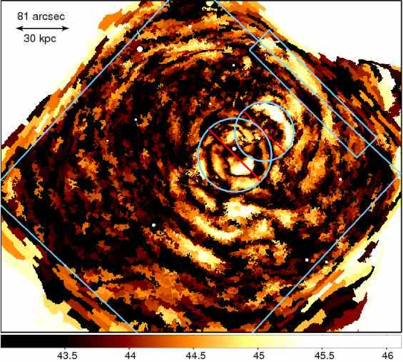
Figure 4: Power in surface brightness fluctuations, assuming they are due to spherical waves. The units are $\mathrm{log}_{10}\hbox{$\rm\thinspace erg\rm\thinspace s^{-1}\,$}$. The rectangles show the regions examined in Fig. 5 and 6. The circles show the excluded inner bubble and NW bubble regions. We assume a factor of 2.5 to convert from surface brightness to density variations.

For each pixel on the fractional surface brightness variation map, we compute the power in a spherical wave from Equation 2, assuming that the radius of the wave is the projected radius on the sky. Deprojected density and temperature values at each radius were calculated from a fit to the average profiles in Sanders et al. (2004). In Fig. 4 we show a map of computed power values for each pixel, assuming a factor of 2 to convert from surface brightness variations to density variations. Many of the ripple features in Fig. 1 (right panel) are seen in this image, plus the radio bubbles (which are not themselves sound waves). We bin the data in this image rather than use simple smoothing, as noise in the outer regions means that the power is overestimated.

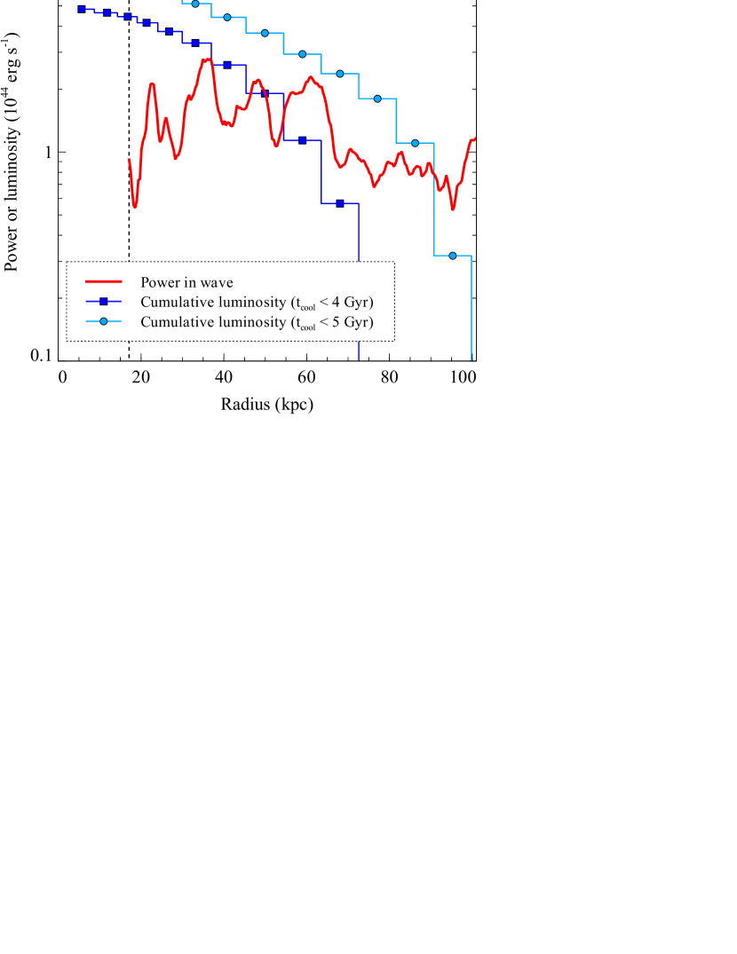
Figure 5: Plot of mean power in sound waves and the cluster cumulative X-ray luminosity inwards of where the cooling time is 4 or 5 Gyr. The vertical line shows the inner radius of our measurements due to the radio lobes. The total power in the lobes approaches $10^{45}\hbox{$\rm\thinspace erg\rm\thinspace s^{-1}\,$}$ (Dunn & Fabian, 2004).

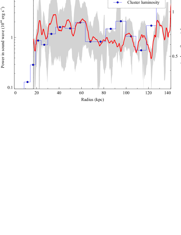
Figure 6: Plot of mean power in sound wave and the cluster luminosity per unit length (in radius). The shaded region shows the the minimum and maximum sound wave power when the data are split into six equal sectors. The cluster luminosity shows the heating rate at each radius required to combat cooling. The vertical line shows the inner radius of our measurements due to the radio lobes. Note the difference in scales, the power being on the left in units of $10^{44}\hbox{$\rm\thinspace erg\rm\thinspace s^{-1}\,$}$ and the luminosity on the right in units of $10^{43}\hbox{$\rm\thinspace erg\rm\thinspace s^{-1}\,$}\rm\thinspace kpc^{-1}$.

In Fig. 5 we show the average values at each radius, masking out the central bubbles and north-west bubbles and the edges of the CCD to avoid filtering artifacts (using the regions in Fig. 4). On the plot we also display the cumulative luminosity from the cluster calculated from the deprojected density, temperature and abundance values from Sanders et al. (2004). We accumulate the luminosity inwards from a radius of 75 or 100 kpc, the radii corresponding to where the mean radiative cooling time of the gas (Sanders et al., 2004) is $\sim 4$ or $5\rm\thinspace Gyr$, the likely age of the cluster. Note that if the sound speed is a function of azimuth in the cluster (the temperature map indicates that this is so), then the phasing of the waves depends on azimuth. This will lead to smearing of the ripples in Fig. 5.

We plot the wave power out to larger radii in Fig. 6. In this graph we also show the variation in wave power at each radius as a shaded region. This was computed by repeating the calculation of the average power in six equal sectors, and shading the region between the minimum and maximum values at each radius. At large radii only a couple of sectors were used, due to the position of the source on the detector. We show the luminosity of the cluster per unit length of radius in this plot to compare to the wave power.

Fig. 5 shows that the net power in the ripples is a few times $10^{44}\hbox{$\rm\thinspace erg\rm\thinspace s^{-1}\,$}$ and sufficient to offset a significant part of the radiative cooling within the innermost 70 kpc or so. The power implied by the analysis drops off with radius out to 120 kpc, with an e-folding length of about 50 kpc, consistent with models of viscous dissipation (Fabian et al., 2003a), which is required if heating by sound waves offsets radiative cooling.

Larger power is seen near the edge of Fig. 6 around 105, 115 and 125 kpc radius. These show possible evidence that the source was more powerful several $10^{8}\rm\thinspace yr$ ago. Such powerful shocks could have been created as several individual bursts, or from a single burst producing multiple sound waves (Brüggen et al., 2007). We caution that most of the signal comes from a small angular region to the extreme SW of the main detector. Further observations covering a wider region are required to accurately determine the wave power at this radius.

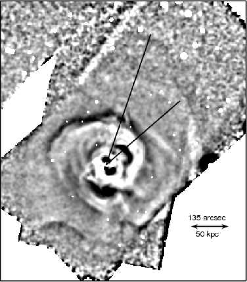
Figure 7: Further possible surface brightness discontinuities to the north of the cluster. This is an unsharp-masked image, subtracting images smoothed with a Gaussian by 4 and 16 arcsec and dividing by the 16 arcsec map. Point sources were excluded from the smoothing. The apparent features are at radii of $\sim 130$ and 170 kpc (indicated by solid lines).

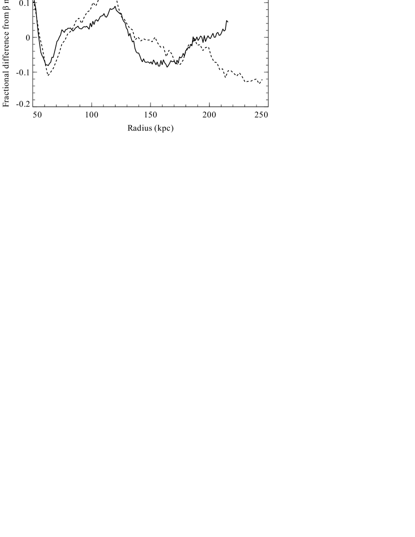
Figure 8: Fractional residuals from a $\beta$ model fit to the surface brightness in sectors to the north at large radii. The full sector shows a profile between 19 and $75^{\circ}$ from west towards north, while the narrow sector is between 59 and $75^{\circ}$.

We also looked for structure in images of the cluster combining all of the ACIS (Advanced CCD Imaging Spectrometer) CCDs. Fig. 7 shows an unsharp-masked image of the north of the cluster to large radii. We note that there appears to be a sharp edge at around 130 kpc radius in this direction (although it varies in radius in the northern sector). This is at approximately the same radius as the ripple seen in Fig. 6. The edge can be seen in residuals from $\beta$ model plus background fits to a wide and narrow sector (Fig. 8). This discontinuity can also be seen in an XMM-Newton observation of Perseus (Fig. 7 in Churazov et al. 2003).

At a radius of around 170 kpc is another feature. This appears to be a dip in surface brightness followed by a rise. This feature is particularly sharp in fits to the surface brightness in a narrow sector (Fig. 8). A possible interpretation is an ancient radio bubble which is still intact. The thermal gas pressure is likely to be around 4 times less at this radius, so if the bubble remains intact it will be around 4 times larger than it was originally (if it retains its original energy). Rough scaling with the rising bubble NW of the nucleus suggests that it would have to have at least twice as much energy. The direction from the centre in which the dip is most visible (the longer solid line in Fig. 7) is also directly along the northern H$\alpha$ filament and fountain (Fabian et al., 2006). If it is indeed a bubble then it shows that bubbles remain intact to very large radii in galaxy clusters. Bubble-like low pressure regions were also seen to the south of the core (Fabian et al., 2006).

To constrain better the power in the feature at 130 kpc and confirm the radio bubble near 170 kpc radius, requires further deep observations by Chandra offset from the cluster core to improve the point spread function (the average radius of which is 10 arcsec at 10 arcmin off axis, compared with $\sim 1$ arcsec on axis).

4 Metallicity map

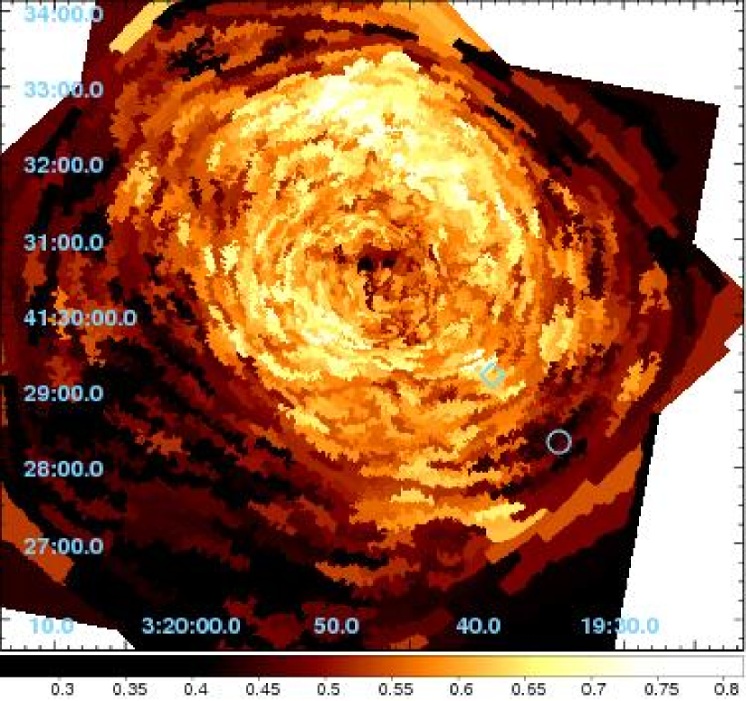
Figure 9: Metallicity map of the core of the cluster relative to solar. Regions contain greater than $4\times 10^{4}$ counts. Fits assume solar ratios of elements, but the results mainly depend on the iron abundance. Uncertainties for each spectral fit range smoothly from $0.025$ in the centre to $0.07\hbox{$\thinspace\mathrm{Z}_{\odot}$}$ to the extreme bottom left of this image. The circle shows the approximate position of the ancient bubble, and the diamond shows the high metallicity blob in its apparent wake.

Fig. 9 shows a metallicity map of the core of the cluster. This was generated by extracting spectra from contour-binned regions (Sanders, 2006) containing $\sim 4\times 10^{4}$ counts. The spectra were fit by a phabs absorbed mekal model with the absorption, temperature, emission-measure and metallicity free. Note that the plot does not clearly show the high abundance shell (possibly marking the location of an ancient bubble) found by Sanders et al. (2005) as there were no new data in that region in these observations, and the spatial regions we use here are larger.

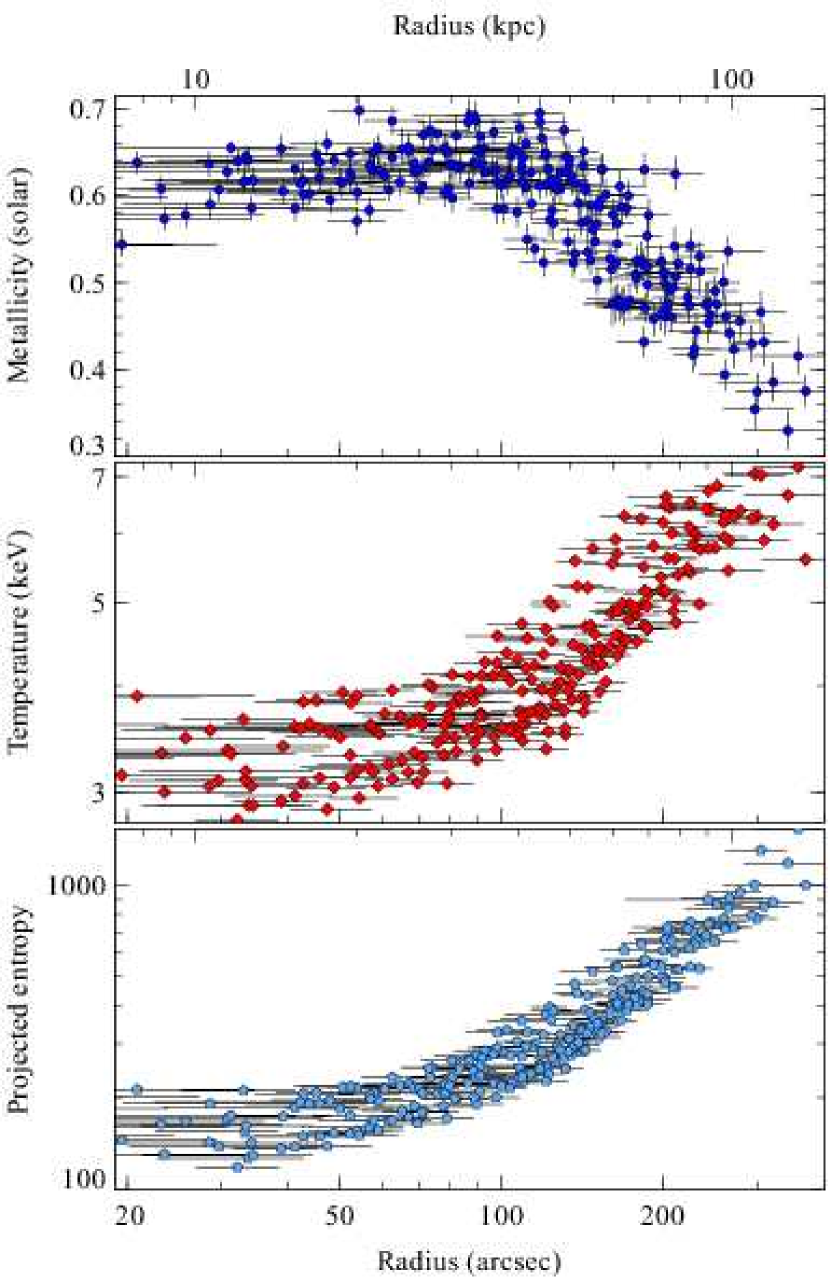
Figure 10: Radius versus projected temperature and metallicity. Values were measured from spectral fitting a mekal model to spectra from bins with $\sim 2.5\times 10^{5}$ counts. Also plotted is the projected entropy as a function of radius (see Section 4.1).

To examine the variation more quantitatively, we have repeated the spectral fitting using regions containing $\sim 2.5\times 10^{5}$ counts to decrease the size of the uncertainties. The radial temperature and metallicity variation are plotted in Fig. 10, generated by plotting the average radius of each bin against the value obtained from that region. At each radius there is a large spread in temperature and abundance.

4.1 Metallicity relations

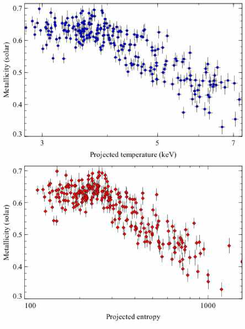
Figure 11: Temperature versus metallicity and pseudo-entropy versus metallicity plots. All values are projected. The bins used are the same as in Fig. 10.

In Sanders et al. (2004) we plotted the temperature of regions against their metallicity. As the temperature of the gas declines towards the centre, the metallicity reaches a maximum at a radius of 40 kpc, then decreases again. We plot the metallicity-temperature relation from the new data in Fig. 11 (top panel). Although we see a similar relation, the reduced errors bars show that there is significant metallicity scatter at each temperature. Indeed the scatter appears similar to that in the radial plot of the metallicity (Fig. 10). The temperature of the gas does not appear to correlate better with the metallicity than the radius.

Another interesting physical quantity is the entropy of the gas. Entropy in clusters is usually defined as $K=kTn_{e}^{-2/3}$. Using the xspec normalisation per unit area on the sky, $N\propto n_{e}^{2}d$, where $d$ is a depth in the cluster, which we assume to be constant, we can calculate a pseduo-projected entropy quantity $N^{-1/3}kT$. The plot of this quantity against the metallicity (Fig. 11 bottom panel) looks similar to the temperature-metallicity plot, with a great deal of scatter at each entropy value. The values use $N$ in xspec normalisation units per square arcsec and $kT$ in keV.

The scatter in the abundance seems unrelated to the temperature, radius, or entropy. Higher metallicity regions will have shorter mean radiative cooling times as the line emission is stronger, but this effect is not strong at temperatures of $\sim 3-7\rm\thinspace keV$, so it is perhaps not surprising that metallicity and temperature or entropy (and therefore cooling time) are unrelated.

4.2 Central abundance drop

There is also a drop in metallicity in the central regions (as can be seen in the metallicity map in Fig. 9). This feature appears to be unaffected by including other components, such as extra temperature components, or powerlaw models.

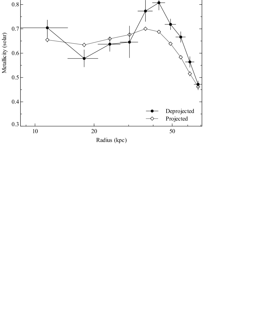
Figure 12: Iron metallicity profile to the NW of the cluster between position angles 290.0 and $4.7^{\circ}$ from 3C 84. This was produced by fitting vmekal models to projected and deprojected spectra.

We have investigated whether the central drop in metallicity could be caused by projection effects. We use the spectral deprojection method outlined in Appendix A to construct a set of deprojected spectra. Fig. 12 shows the iron metallicity profile computed by fitting isothermal vmekal models to the spectra before and after deprojection. In the fit the elemental abundances of O, Ne, Mg, Si, S, Ar, Ca, Fe and Ni were allowed to vary, with the gas temperature, the model emission measure, and the absorbing column density. The analysis shows the peak at around 40 kpc radius is enhanced by accounting for projection and the central drop remains.

The drop in metallicity in the central regions appears to be robust. The entropy of the gas in the central regions is much lower than further out, which means it is difficult for the source of the low metallicity gas to be from larger radius.

4.3 Small scale variation

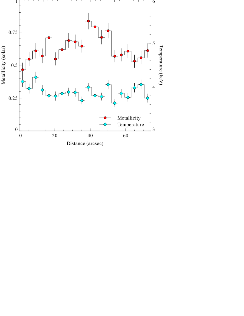
Figure 13: Abundance and temperature profiles across the high metallicity blob near 3$\aas@@fstack{h}$19$\aas@@fstack{m}$40$\aas@@fstack{s}$, $+41^{\circ}29^{\prime}15^{\prime\prime}$. The profile crosses the blob in the SE to NW direction, inclined by an angle of $40^{\circ}$ from the west northwards.

Much of the structure in the metallicity map is real. To demonstrate this, we show in Fig. 13 a metallicity and temperature profile across the high metallicity blob apparently in the wake of a possible ancient bubble down to the extreme SW (marked on Fig. 9; Sanders et al. 2005). The metallicity profile shows a significant peak with a width of $\sim 5\rm\thinspace kpc$ at the position of the blob (we also see $\sim 5\rm\thinspace kpc$ metallicity features near the filaments in Section 6). There is no obvious correlation between the temperature and metallicity profiles. Taking the global diffusion coefficient of $2\times 10^{29}\rm\thinspace cm^{2}\rm\thinspace s^{-1}$ measured by Rebusco et al. (2005) in Perseus and a lengthscale of 5 kpc, the lifetime of such a feature is only $\sim 40$ Myr. This is roughly comparable to the buoyancy timescale estimated for the ancient bubble of 100 Myr (Dunn et al., 2006), given the large uncertainties, but may require that diffusion is suppressed on small scales as it appears unlikely that the metals could have been injected in-situ. The sharp edges of the feature would imply diffusion times of only a few Myr, requiring significant suppression.

The blob has a metallicity approximately $0.2\hbox{$\thinspace\mathrm{Z}_{\odot}$}$ higher than its surroundings (which are at approximately $0.6\hbox{$\thinspace\mathrm{Z}_{\odot}$}$). This is probably a lower limit because of projection effects. Assuming the blob is sphere with diameter 5 kpc, and a local electron density of around $0.037\hbox{$\rm\thinspace cm^{-3}\,$}$ (Sanders et al., 2004), it represents an enhancement of around $2.6\times 10^{4}\hbox{$\rm\thinspace M_{\odot}$}$ of Fe. If most of this enrichment is due to Type Ia supernova, then this corresponds to around $3.7\times 10^{4}$ supernova (assuming $0.7\hbox{$\rm\thinspace M_{\odot}$}$ of Fe produced per supernova). Taking the timescale from diffusion, this corresponds to 0.1 supernova type Ia per century for this 5 kpc radius region, which is a significant fraction of the rate expected from a single galaxy.

5 The high velocity system

Gillmon et al. (2004) studied the High Velocity System (HVS), a distinct emission-line system at a higher velocity than NGC 1275 (Minkowski, 1957), using an earlier 200-ks Chandra observation of the system. The system is observed in absorption in X-rays (Fabian et al., 2000), as it lies between most or all of the cluster and the observer. Gillmon et al. (2004) mapped the absorbing column density and placed a lower limit of 57 kpc of the distance between the nucleus of NGC 1275 and the HVS. They obtained a total absorbing gas mass of $1.3\times 10^{9}\hbox{$\rm\thinspace M_{\odot}$}$, assuming Solar metallicities.

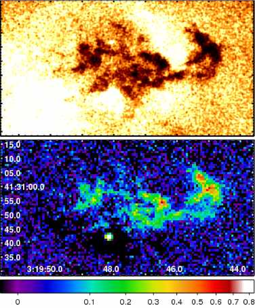
Figure 14: (Top panel) Image of the high-velocity system in the 0.3 to 0.7 keV band smoothed by a Gaussian of 0.49 arcsec. (Bottom panel) Measurements of the equivalent Hydrogen column density over the high-velocity system region, in units of $10^{22}\hbox{$\rm\thinspace cm^{-2}\,$}$ (subtracting Galactic absorption of $0.12\times 10^{22}\hbox{$\rm\thinspace cm^{-2}\,$}$). The values were measured from spectral fitting in $0.74\times 0.74$ arcsec pixels. The central nucleus of 3C 84 shows up as a point-like object near 3$\aas@@fstack{h}$19$\aas@@fstack{m}$48$\aas@@fstack{s}$, $+41^{\circ}30^{\prime}40^{\prime\prime}$. The uncertainty on the column density on individual pixels is around 0.1 for the regions of highest absorption and 0.03 outside of the HVS.

Here we repeat the mapping analysis with the new 900-ks dataset. Fig. 14 (top panel) shows an image in the 0.3-0.7 keV band, clearly showing the absorbing material. To quantify the amount of material we fitted an apec thermal spectral model for the cluster emission, absorbed by a phabs photoelectric absorber to spectra extracted from a grid of $0.74\times 0.74$ arcsec regions around the HVS. In the fits the temperature of the thermal emission, its normalisation, and the absorbing column density were free. The abundance of the thermal gas was fixed to $0.7\hbox{$\thinspace\mathrm{Z}_{\odot}$}$ (based on the results of spectral fitting to larger regions near the core of the cluster; the results are very similar if this is allowed to be free). Spectra were binned to have a minimum of 5 counts per spectral channel. We minimised the C-statistic to find the best fitting parameters (note that no background or correction spectra were used in the fits here, as the cluster is much brighter than the background here).

In Fig. 14 (bottom panel) we show the resulting Hydrogen column density map over the HVS region, including the Galactic contribution. We stress that these values are equivalent Hydrogen column density. The measurements are most sensitive to the abundance of Oxygen in the absorber. The Hydrogen column density is calculated assuming the Solar abundance ratios of Anders & Grevesse (1989), which gives an Oxygen to Hydrogen number density ratio of $8.51\times 10^{-4}$. The column density is flat in this region beyond the HVS. We obtain an average value of this Galactic component of $0.12\times 10^{22}\hbox{$\rm\thinspace cm^{-2}\,$}$, consistently from several surrounding regions.

The total number of absorbing atoms can be calculated using the mean absorption over the HVS, the Galactic contribution, and the distance to Perseus. We converted this into a total absorbing mass of $1.1\times 10^{9}\hbox{$\rm\thinspace M_{\odot}$}$, assuming Solar metallicity ratios. This is lower than the value of $(1.32\pm 0.05)\times 10^{9}\hbox{$\rm\thinspace M_{\odot}$}$ quoted by Gillmon et al.. We repeated our analysis using the 1.96 arcsec binning factor used in that paper, but this did not significantly change our result. The twenty per cent difference may be due to the different calibration used in the earlier analysis, particularly the lack of correction for the variation in the contaminant on the detector, as the Galactic value is important to determine the total mass.

To place an improved lower limit of the distance of the HVS from the cluster nucleus, we examined a 0.3 to 0.7 keV image, where the absorption is strongest. Taking 1-1.5 arcsec diameter regions (with total area 3.9 arcsec²) in the three highest absorption regions we find 17 counts in total in this band. Exposure-map correcting this surface brightness, and comparing it to the exposure-map corrected image of the cluster, we find that the surface brightness from the cluster only goes down to this level at a radius of approximately 110 kpc. This is a lower limit of the distance of the HVS from the cluster centre, as if the HVS were closer, the cluster emission should be ‘filling in’ the decrement in count rate caused by the absorption (Gillmon et al., 2004). This lower limit is a significantly better the previous value of 57 kpc.

As we discuss in Section 7.1.1, the HVS could have a shock cone behind it if it is travelling exactly along our line of sight towards the cluster. If this is the case, the shocked material would have a significantly lower density than the cluster at the same radius. This would mean that the lower limit we compute above would be overestimated.

6 Profiles across filaments

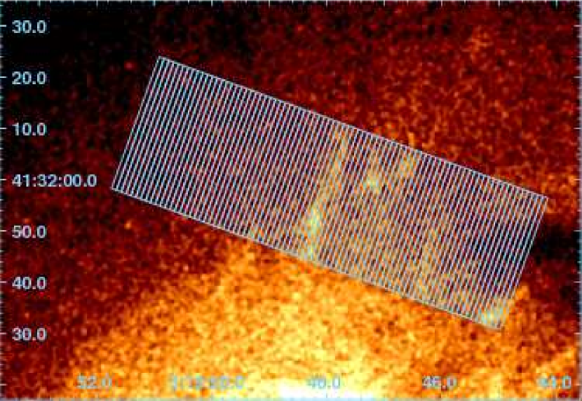
Figure 15: Location of the regions used to measure the thermal properties across the filaments, displayed on a 0.3 to 1 keV image. Each of the 80 regions is $1\times 27.3$ arcsec in size.

To investigate the thermal structure of the X-ray filaments associated with the H$\alpha$ nebula in detail, we extracted spectra from small $1\times 27.3$ arcsec boxes in a profile across the filament (the regions we used are shown in Fig. 15). We created background spectra, responses, ancillary responses, and out of time background spectra for each region.

Figure 16: Emission measure profiles across the filaments in the different temperature components. The top panel shows an unsharp-masked 0.5-7 keV X-ray image rotated so that the bins lie across it. The second panel shows a similar H$\alpha$ image. The next panels show the 0.5, 1, 2 and 4 keV temperature component xspec normalisations, measured from the 1 arcsec wide bins. The final panels show the best fitting absorbing Hydrogen column density and the metallicity of thermal components.

6.1 Multiphase model

Our first model was to fit the spectra with a multiphase model consisting of apec thermal components at fixed temperatures of 0.5, 1, 2, 4 and 8 keV. The normalisations were allowed to vary and the metallicities of each of the components were tied together. They were absorbed with a phabs photoelectric absorber which was allowed to vary. We assume each component has the same metallicity as we cannot measure them independently. The measurement is likely to be driven by the cooler components as they are line-dominated. The model is similar to that used to produce figure 12 in Fabian et al. (2006), mapping the multiphase gas. We show the emission measure of each temperature component in Fig. 16, with the absorbing column density and metallicity. Also shown is an unsharp-masked image of the region examined in the 0.5-7 keV X-ray band (the X-ray image has been rotated so that the 1-arcsec bins lie horizontally across the region) and the H$\alpha$ image from Conselice et al. (2001) taken using the WIYN telescope. We chose the rotation angle so that the bins were lined up across the central X-ray features. The H$\alpha$ filaments are not quite aligned in angle.

The plot shows that the filaments do not contain gas at temperatures of $\sim 4$ keV. At 2 keV we start to see the filaments, although their signal is fairly weak against that from nearby gas. The filaments are very strong near 1 keV, and still visible at 0.5 keV. There are some point-to-point differences however. The strong filament at 39 arcsec distance is strong in 1 and 0.5 keV, but the one nearby 46 arcsec does not appear at 1 keV, but does at 2 and 0.5 keV.

The column density profile is fairly flat. A linear model fitted to the column density profile gives a reduced $\chi^{2}$ of $86/78=1.10$. We see no evidence for additional X-ray absorption associated with the filaments.

The metallicity profile shows several features, which matches the complex structure seen in the metallicity map (Fig. 9). A simple linear fit gives a reduced $\chi^{2}$ of $105/78=1.34$. There are quite strong peaks at the 59 arcsec, and at 12 arcsec. Neither is exactly at the position of a filament, though the one at 59 arcsec is offset by an arcsec or two from some gas from 2 to 0.5 keV. It is possible that some of the metallicity variation is caused by incomplete modelling of the multiphase gas within the filaments, but we observe almost identical variation with single phase and cooling flow (below) models. All models assume that the gas at each temperature has the same metallicity, though the cooler gas will dominate in the measurement of the metallicity.

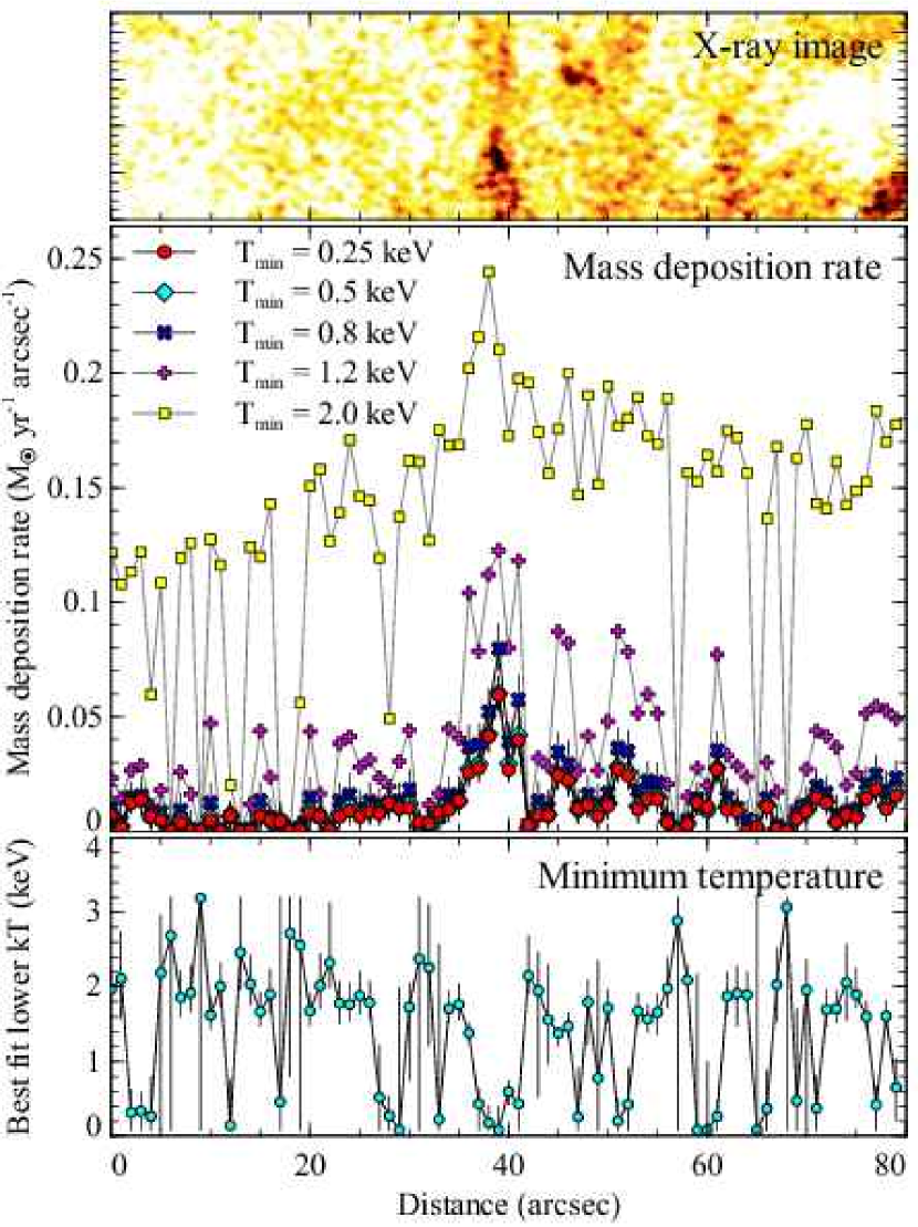
Figure 17: Results of fitting a cooling flow model to spectra extracted across the filaments in Fig. 15. The top panel shows an image of the region. In the second is plotted the mass deposition rates per bin obtained by fixing the lower temperature of the cooling flow models to certain values. The bottom panel shows the best fitting lower temperature if it is allowed to be free.

6.2 Cooling flow model

Given the range in the temperature in the filaments, we try fitting a cooling flow model to the spectra, as the gas may be cooling within the filament. We used the isobaric mkcflow model, which models cooling between two temperatures at a certain metallicity and gives the normalisation as a mass deposition rate, plus a mekal single phase thermal component. The upper temperature of the cooling flow component was tied to the temperature of the thermal component, and the metallicities were also tied. Both components were absorbed by a phabs absorber. Fig. 17 shows the mass deposition rates obtained with fixed minimum temperatures. The 0.25 keV rate is equivalent to a traditional cooling flow where the gas cools out of the X-ray band, while the others are truncated cooling flows. Also plotted is the best fitting minimum temperature if it is allowed to vary.

The results show that within the filaments, the model adds increasing amounts of the cooling flow component, indicating a range of temperatures. Using a cooling flow component with a 0.25 keV minimum temperature, the emission measure of the single phase thermal component varies relatively smoothly over the region. There is less apparent cooling as the minimum temperature decreases (as with the results of Peterson et al. 2003), until below $\sim 0.8\rm\thinspace keV$ where the results are approximately consistent. If the gas is actually cooling in these filaments, these results indicate a rate of $\sim 0.25\hbox{$\hbox{$\rm\thinspace M_{\odot}$}\rm\thinspace yr^{-1}\,$}$ in the central filament in this small region examined. All of the $\sim 0.5\rm\thinspace keV$ X-ray emitting gas observed in the Perseus cluster appears to be associated with the H$\alpha$ emitting filaments or is close to the nucleus (Fabian et al., 2006). The lower gas temperature measured here is consistent with zero in the centres of the filaments, but appears to increase by a few arcsec. We note that the best fitting absorbing column density is almost identical to the values from the multiphase model in Fig. 16, so no additional absorption is required.

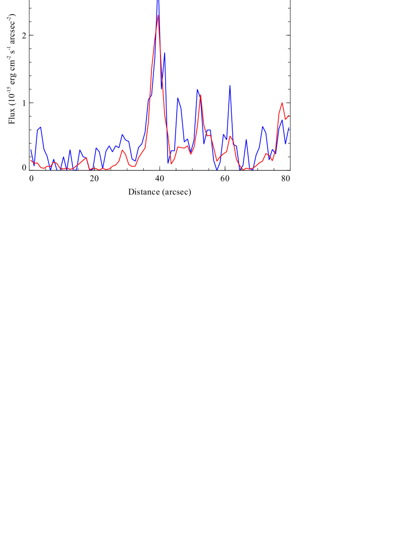
Figure 18: Comparison of H$\alpha$ surface brightness flux profile across the filaments (using data from Conselice et al. 2001) versus unabsorbed 0.001 to 30 keV surface brightness flux from the cooling flow model cooling down to 0.25 keV. Cooling to 0.0808 keV, the minimum available, increases the results by about 5 per cent. Both of these fluxes are in the same units.

In Fig. 18 we compare the flux from the cooling flow component cooling down to 0.25 keV (above) against the flux in the continuum-subtracted H$\alpha$ waveband from the data from Conselice et al. (2001) (using the fluxes given in several regions to calibrate the count to flux scale). The H$\alpha$ filter used had a central wavelength of 6690 A and a FWHM of 77 A, and the fluxes have been corrected for Galactic extinction, and includes N ii emission. The plot shows that the X-ray flux of the filaments, assuming a cooling flow model, is very close to the H$\alpha$+N [ii] flux for most of the filaments. The flux from the multitemperature model (Fig. 16) is somewhat similar to that from the cooling flow model. If the 2, 4 and 8 keV components are ignored, the flux is smaller by a factor of $\sim 4$ than the cooling flow flux, but including the 2 keV flux boosts this to well above this value.

6.3 Filament geometry

If the gas in a filament is in pressure equilibrium with its surroundings, the pressure is known and thus is the temperature of the gas in the filament, so we can estimate the volume of the emitting region.

We fitted a simple absorbed two-temperature mekal spectral model to the $1\times 27.3$ arcsec bin at 38 arcsec offset where the filaments are strongest (see Fig. 16). The best fitting temperatures from the spectral fit are $0.69\pm 0.05$ and $3.36\pm 0.09$ keV, corresponding to the temperature of the filament and its surroundings, respectively, under the assumption that the gas has a single temperature in the filament. Taking the emission measure of the filament component and an electron pressure of $0.128\rm\thinspace keV\rm\thinspace cm^{-3}$ (from the deprojected values in Sanders et al. 2004, Fig. 19), then the volume of the emitting region is $1.0\times 10^{63}\rm\thinspace cm^{3}$. The extracted region on the sky is $0.37\times 10.2\rm\thinspace kpc$. If we assume the filament is a cuboid with the facing side of the dimensions given, we calculate a depth of 9 pc. If the filament is a single long and thin tube with length 10.2 kpc, it would have dimensions of $\sim 60\rm\thinspace pc$ across.

The lack of depth shows the filament is unlikely to be a sheet viewed from the side, and the disparity with the other dimensions suggests that the filament is in fact made up of small unresolved knots of X-ray emission. If there were $10^{3}$ such blobs, they would have dimensions of $\sim 30$ pc.

6.4 Flux emitted from the filament

Taking the volume above for the filament in the 38 arcsec bin and assuming pressure equilibrium implies there are $\sim 1.9\times 10^{62}$ electrons in the cooler filamentary component. The difference in temperature of the cooling X-ray emitting gas from the surrounding gas is $\sim 2.7\rm\thinspace keV$. This implies there would be $\sim 2.5\times 10^{54}\rm\thinspace erg$ released if the X-ray emitting filament was to cool out of the surrounding intracluster medium (assuming twice the number of particles as electrons and $3/2\>kT$ energy per particle, which does not include any work done by the surroundings on the cooling filament).

The luminosity of the bin in the H$\alpha$ waveband is $6\times 10^{40}\hbox{$\rm\thinspace erg\rm\thinspace s^{-1}\,$}$. This can be multiplied by a factor of 20 to account for other line emission, for example Ly$\alpha$. Therefore if the line emission is powered by cooling out of the intracluster medium, the timescale for this process is $\sim 7\times 10^{4}$ yr. The dynamical timescale for a 30 pc region, assuming a sound speed of $300\hbox{$\rm\thinspace km\rm\thinspace s^{-1}\,$}$, would be $\sim 10^{5}\rm\thinspace yr$, so it is approximately possible for the cooling medium to be replenished.

Conduction of heat from the surrounding intracluster medium may also be able to power the filaments. For a 2 keV plasma, the Spitzer (1962) conductivity is $\sim 9\times 10^{11}\hbox{$\rm\thinspace erg\rm\thinspace s^{-1}\,$}\rm\thinspace cm^{-1}\rm\thinspace K^{-1}$. If we assume a geometry of a 30 pc wide tube which is 10.2 kpc long and if the heat is being conducted between 3.4 and 0.7 keV over 30 pc, this corresponds to a heat flux of $\sim 5\times 10^{42}\hbox{$\rm\thinspace erg\rm\thinspace s^{-1}\,$}$. Such a flux is sufficient to fuel the line emission. It however depends greatly on the assumed conductivity (which depends on temperature to the 5/2 power) and geometry (Böhringer & Fabian, 1989; Nipoti & Binney, 2004). To provide the energy for the line emission, the heat must be able to travel to presumably smaller and cooler regions than that of the the 0.7 keV gas, which conductivity makes it increasingly hard to do. Note that any conduction model requires that the surrounding soft X-ray emitting gas and the filament have a low relative velocity. If conduction is too efficient at transporting heat the filament will evaporate, leading to a certain critical minimum size for growth (Böhringer & Fabian, 1989), which depends on how much conduction is suppressed and the temperature and density of the surrounding ICM.

7 Hard X-ray emission

As discussed in the introduction, Sanders et al. (2004) found evidence for a distributed hard component surrounding the core of the cluster by fitting a multitemperature model with a 16 keV component. The total 2-10 keV luminosity of this hard component is $\sim 5\times 10^{43}\hbox{$\rm\thinspace erg\rm\thinspace s^{-1}\,$}$. Later Sanders et al. (2005) used a thermal plus powerlaw model to fit the data giving a similar flux. This hard component has been confirmed with XMM-Newton data (Molendi, private communication). Assuming this emission is the result of inverse Compton scattering of IR and CMB photons by the population of electrons which also emit the observed radio, the magnetic field over the core of the cluster was mapped.

Here we examine the hard flux from the cluster using this very deep set of observations, and investigate the effect of different spectral models. We binned the data using the contour binning algorithm with a signal to noise of 500 ($\sim 2.5\times 10^{5}$ counts in each bin).

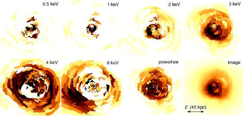
Figure 19: Results from the multitemperature plus $\Gamma=2$ powerlaw fits to regions containing $\sim 2.5\times 10^{5}$ counts. The images show the emission measures per unit area for each of the components, and finally the broad band Chandra image of the same region.

Our first model is a multitemperature model made of different temperature components plus a powerlaw to account for the hard emission. This is a more complex model than that used by Sanders et al. (2005), as we wished to account for the known cool gas in the cluster which may affect the powerlaw signal if not modelled correctly. Hotter gas projected from larger radii in the cluster can also give a false signal. The data were fitted using a model made up of apec thermal components at fixed temperatures of 0.5, 1, 2, 3, 4 and 8 keV, plus a $\Gamma=2$ powerlaw, all absorbed by a phabs photoelectric absorber. The normalisations of the components were allowed to vary, the metallicities tied to the same free value, and the absorption was free. We used a $\Gamma=2$ powerlaw here as this is close to the best fitting photon index of the radio emission (Sijbring, 1993), and the best fitting X-ray spectral index in the core (Sanders et al., 2005). Fig. 19 shows the emission measure per unit area for each of the thermal components, the powerlaw normalisation per unit area, and the broad band Chandra image of the same region.

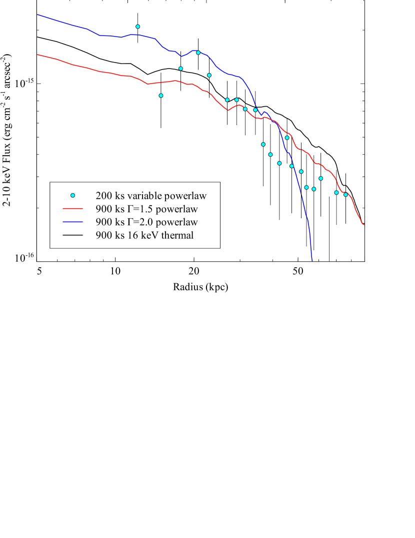
Figure 20: Flux per unit area on the sky for multicomponent models plus powerlaws or plus a hot 16 keV component. Also plotted are the background-subtracted results from an earlier analysis (Sanders et al., 2005).

The thermal gas maps show similar distributions to the earlier analyses with smaller uncertainties (Sanders et al., 2004; Fabian et al., 2006). We plot the radial profile of the 2-10 keV flux of the powerlaw component in Fig. 20. Also shown is the radial profile for a $\Gamma=1.5$ powerlaw instead of the $\Gamma=2$ powerlaw, or a 16 keV thermal component, and the older results from Sanders et al. (2005) (after subtracting the estimated ‘background’ from hot projected thermal gas). The total emitted flux from each of the models is fairly consistent, except at large radii where the signal is low. Hot thermal gas, as expected, gives similar results to a $\Gamma=1.5$ powerlaw. The best fitting powerlaw index looks similar to the results in Sanders et al. (2005), with a transition of $\Gamma\sim 2.2$ powerlaw in the centre to $\Gamma\sim 1.4$ in the outskirts.

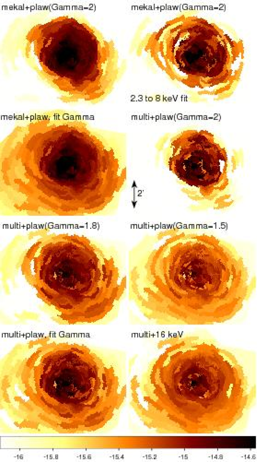
Figure 21: Fluxes for the powerlaw or hot thermal components for various models. The units are $\mathrm{log}_{10}\,\hbox{$\rm\thinspace erg\rm\thinspace cm^{-2}\rm\thinspace s^{-1}\,$}$, in the 2–10 keV band. The panels show, from left to right, top to bottom, (1) fitting a thermal mekal plus a $\Gamma=2$ powerlaw from 0.6 to 8 keV, (2) only fitting it between 2.3 and 8 keV, (3) allowing the $\Gamma$ to vary from 1.4 to 2.4, (4) multicomponent thermal apec model plus a $\Gamma=2$ powerlaw, (5) using $\Gamma=1.8$, (6) using $\Gamma=1.5$, (7) allowing $\Gamma$ to vary between 1.4 and 2.4, and (8) multicomponent thermal apec model plus 16 keV component.

We map the distribution of hard flux per unit area for a variety of different models in Fig. 21. We show the variation of flux (top left) just using a single thermal model plus powerlaw (as in Sanders et al. 2005), (top right) fitting that model just in the high energy band, and (second row left) allowing the powerlaw index to vary. We also show the results (second row right, and third row) from multitemperature plus powerlaw models with $\Gamma=2,1.8$ and 1.5, and (bottom left) fitting for the index. Finally we show the result (bottom right) using a multitemperature model including a 16 keV hard component.

There are problems with steep powerlaw components as they predict significant extra flux at low X-ray energies. Such flux is not observed, and therefore the best fitting photoelectric absorption increases in the central regions where the powerlaw is strong. It is possible that there is excess absorption in the central regions, but the flux of the powerlaw is very closely correlated with the absorption, so some physical connection between the two would be required. Presumably the non-thermal emission process would need to be dependent on absorbing material, which appears unlikely.

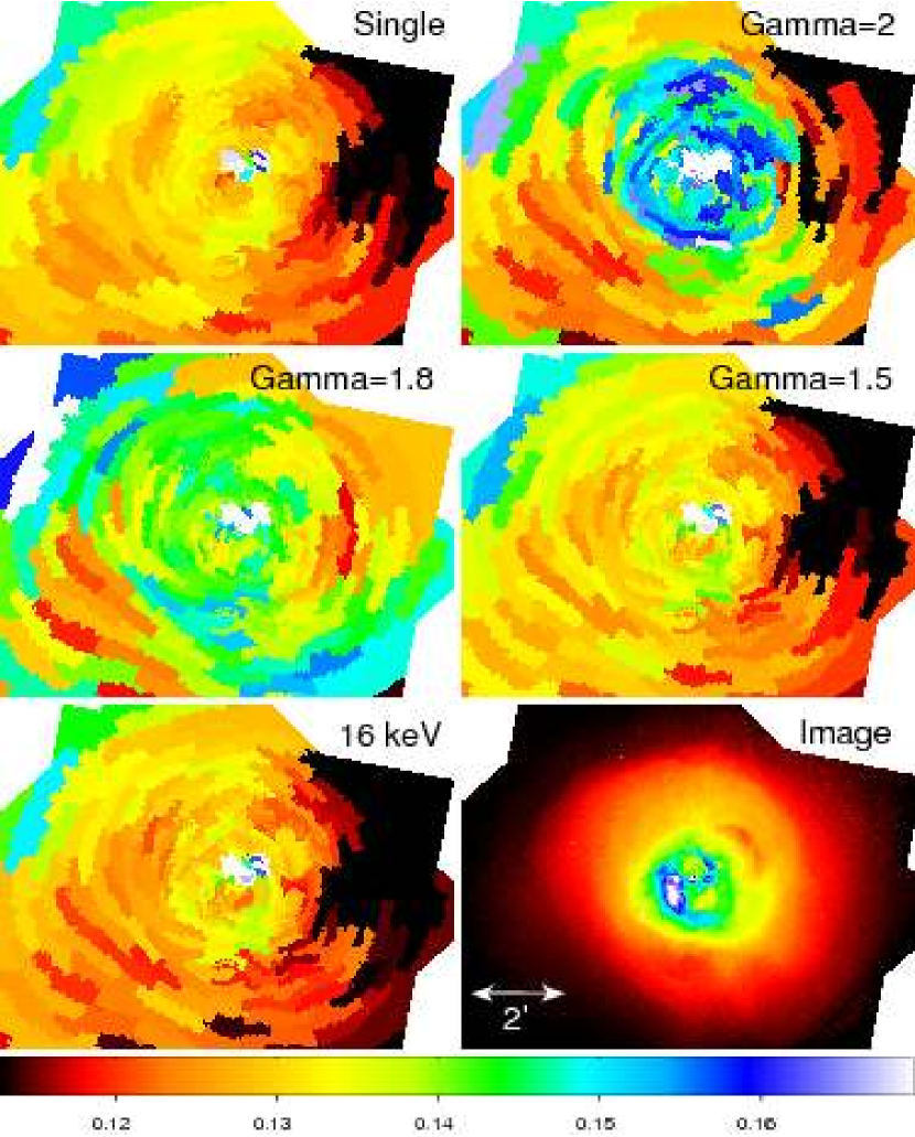
Figure 22: $N_{\mathrm{H}}$ column density maps in units of $10^{22}\hbox{$\rm\thinspace cm^{-2}\,$}$ generated by fitting different spectral models to regions containing a signal to noise ratio of 500. Also shown is an X-ray image of the same area. ‘Single’ shows the results of fitting a single phabs absorbed mekal. ‘Gamma=2, 1.8 and 1.5’ shows the results fitting a multitemperature model plus a powerlaw of the photon index given. ‘16 keV’ shows the results using a multitemperature model including a 16 keV hot thermal component.

Fig. 22 shows the absorption distribution for different models. The top-left panel shows the distribution from fitting a single mekal plasma to the projected spectra. There is obvious variation across the image. Some of this variation may be due to the buildup of contaminant on the ACIS detector, but the current calibration should account for this in the creation of ancillary response matrices. Probably most of the variation is because the cluster lies close to the Galactic plane ($b\sim-13^{\circ}$). If the image is aligned to Galactic coordinates, the variation is mostly in Galactic latitude.

Fitting using a multitemperature model plus a $\Gamma=1.5$ powerlaw or 16 keV thermal component produces absorption maps very similar to the single temperature map. These models require no additional absorption. The $\Gamma=1.8$ requires moderate additional absorption, and $\Gamma=2$ produces absorption clearly correlated to the powerlaw flux (Fig. 21 centre-top row, right column).

Figure 23: Spectrum showing the effect of the 16 keV component to spectral fit. The spectrum shown is a region around 1.8 arcmin north from the nucleus containing $\sim 2.5\times 10^{5}$ counts. The solid line in the top panel is the model, after removing the 16 keV component. The bottom panel is the ratio of the data to the model not including the hard component.

To demonstrate the effect of the hard component on the spectral fit, we show in Fig. 23 the contribution of the hard component to the best fitting model to a spectrum from a region around 1.8 arcmin north of the nucleus. For a 16 keV component the effect is around 10 per cent at low energies, increasing to fifty per cent at high energies: the hard component is about one third or more flux above 4 keV.

7.1 Origin of the hard emission

If we assume that the hard component is real and not an instrumental or modelling artifact, there are two sets of possible emission mechanisms, thermal or non-thermal. If it is non-thermal emission it is likely to be inverse Compton emission from CMB or IR photons being scattered by relativistic electrons in the ICM (Sanders et al., 2005). Another possible origin is hot thermal gas. The probable origin of such material in the cluster is from a shock, and the obvious candidate is the HVS.

7.1.1 Thermal origin: merger of HVS

From Section 5, the HVS lies at minimum distance from the cluster core of 110 kpc, where the electron density of the gas is $\sim 5\times 10^{-3}\hbox{$\rm\thinspace cm^{-3}\,$}$ (Sanders et al., 2004). The HVS is moving at $3000\hbox{$\rm\thinspace km\rm\thinspace s^{-1}\,$}$ relative to the main NGC 1275 system along the line of sight to the observer (Minkowski, 1957). Assuming a 5 keV plasma for the cluster, and that the galaxy is travelling along the line of sight, the Mach number of the HVS is around 2.3.

The collision should produce a shocked Mach cone around the HVS. If the HVS lies at its minimum distance from the cluster, using the Rankine-Hugoniot jump conditions, the density of the post-shocked material should be a factor of 2.1 times greater than its surroundings ($n_{e}\sim 10^{-2}\hbox{$\rm\thinspace cm^{-3}\,$}$) and its temperature around 15 keV.

If the origin of the hard component is the shocked material in the cone, and it lies at the minimum distance from the cluster, we can estimate the depth of the cone from the emission measure of the 16 keV component (close to the expected 15 keV temperature) using the density above. The depth we derive from the peak of the emission is between 200-300 kpc. If this is the correct interpretation, the layer of shocked material is extremely large. This number can be reduced significantly if the preshocked material has a higher density, as the depth is inversely proportional to the square of the density. At the previous minimum distance of around $60\rm\thinspace kpc$ from the HVS from the core of the cluster (Gillmon et al., 2004), the minimum depth is only a few kpc, as the density was increased by a factor of 10. If the HVS lies further away than our minimum distance from the cluster core, it becomes much harder for the thermal interpretation to be a plausible explanation. Whether a thermal origin for the hard component is plausible depends on whether our lower limit of the distance from the cluster to the HVS is overestimated (see Section 5).

7.1.2 Non-thermal origin: inverse Compton processes

If the origin of the flux is from inverse Compton emission, there is a large population of relativistic electrons scattering CMB or IR photons. The bright radio emission from the mini radiohalo in the cluster core indicates that there are relativistic electrons, but we cannot directly observe the required $\gamma\sim 1000$ electrons by their synchrotron emission. The powerlaw index of the inverse Compton emission will be the same as the radio emission, if a single population of electrons produces both. We do not know whether there is a single population. There could be a break in the powerlaw index, or a cut-off in the population.

Under the assumption of a single population, we previously estimated the magnetic field in the core of the cluster to be a 0.3-1$\mu$G (Sanders et al., 2005).

There are some potential issues with an inverse Compton explanation. If the source electron population creates a $\Gamma\sim 2$ powerlaw, we require significant amounts of additional absorption in the core of the cluster (Fig. 22), as the powerlaw is significant at low X-ray energies, unless it breaks in the X-ray band. Such absorption is not seen on the X-ray spectrum of the nucleus using XMM (Churazov et al., 2003). The excess absorption is not required with a flatter powerlaw index ($\Gamma\sim 1.5$). However a flat $\Gamma=1.5$ powerlaw will emit significant flux in the hard ($>20$ keV) band.

Hard X-rays were observed from Perseus using HEAO 1 (Primini et al., 1981) in the 20-50 keV band with a photon index of around 1.9. The flux translates to a total luminosity in the 2-10 keV band of around $1.6\times 10^{44}\hbox{$\rm\thinspace erg\rm\thinspace s^{-1}\,$}$ above the thermal emission. This component was found to be variable over a four year timescale. Nevalainen et al. (2004) observed a flux around four times lower than this value using the high energy PDS detector on BeppoSAX. The variable component must be associated with the central nucleus rather than inverse Compton emission. The separation of the nuclear spectrum from any hard component is difficult, particularly if the nucleus varies on short timescales. Nevalainen et al. (2004) concluded that the central nucleus can account for all of the nonthermal emission observed from Perseus using BeppoSAX. More sensitive measurements of the hard flux from, for example, Suzaku are vital to resolve this issue. Observations with higher spatial resolution close in time would help remove uncertainty about the nuclear component.

The cooling time for electrons producing 10 keV electrons from inverse Compton scattering of CMB photons is $\sim 10^{9}$ yr. It is therefore likely that the spectrum could be broken at these energies. Such breaks could reduce the need for increased absorption for steeper powerlaw models here, or reduce the hard X-ray flux for those with flatter spectra.

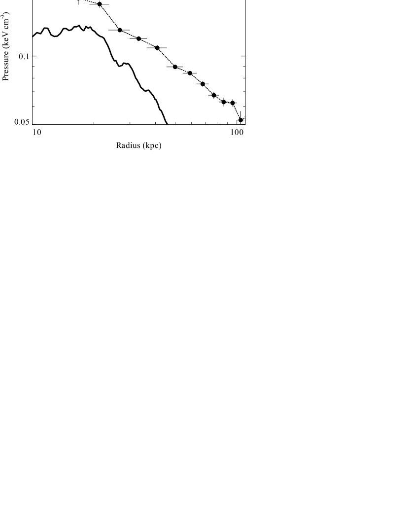
Figure 24: Inferred average nonthermal particle pressure calculated from the $\Gamma=1.5$ powerlaw plus multitemperature results in Fig. 21, assuming inverse Compton emission. Also plotted is the average thermal gas electron pressure from Sanders et al. (2004).

If the emission is the result of inverse Compton emission, the pressure of the relativistic electrons, $P$, is related to the emissivity of the inverse Compton emission, $\mathcal{E}$, by (e.g. Erlund et al. 2006)

$$P=\frac{1}{4}\frac{\mathcal{E}\,m_{\mathrm{e}}\,c}{U\,\gamma\,\sigma_{\mathrm{T}}},$$ (4)

where $U$ is the energy density of the photon field being scattered, $\gamma$ is the Lorentz factor of the electron scattering the photon to the observed waveband, $m_{\mathrm{e}}$ is the rest mass of the electron, $\sigma_{\mathrm{T}}$ is the Thomson cross-section and $c$ is the speed of light in a vacuum. If we assume that the depth of an emitting region in the hard X-ray maps is its radius, and that the X-ray emission is the result of scattering CMB and IR photons (Sanders et al., 2005) we can estimate the nonthermal pressure as a function of radius. We plot this in Fig. 24, showing that the nonthermal pressure is comparable to the thermal pressure near the centre of the cluster.

8 Thermal content of the radio bubbles

Earlier Chandra data have been used to limit the amount of thermal material material within the radio bubbles (Schmidt et al., 2002). This analysis is made more difficult because the geometry of the core of the cluster is complex, and techniques accounting for projection appear not to work generally when examining the bubbles (Sanders et al., 2004). Here we place stringent limits on the volume filling factor of thermal gas using this 900-ks combined dataset using a comparative technique which depends far less on geometry.

We fit the projected spectrum from the inside of the bubble with a model made up of multiple temperature components at relatively low temperatures (fixed to 0.5, 1, 2, 3, 4 and 6 keV with normalisations varied and metallicities tied together) to account for the projected gas, plus a component fixed to a higher temperature to test for the existence of hot thermal gas within the bubble. We also do the fit again with an additional $\Gamma=2$ powerlaw to account for any possible non-thermal emission. We compare the normalisation per unit area of the component accounting for hot thermal gas in the bubble against that from a fit to a neighbouring region at the same radius in the cluster. The temperature of the gas in the bubble is stepped over a range of temperatures in the bubble and comparison regions.

The normalisation per unit area in the bubble and comparison region can be converted into an upper limit on the difference in normalisation per unit area between the two. We use any positive difference between the bubble region normalisation and background, plus twice the uncertainty on the difference (Using the positive uncertainty on the background and the negative uncertainty on the foreground. This is slightly pessimistic compared to symmetrising the errors), to make a 2$\sigma$ upper limit.

Assuming a volume for the bubble, an upper limit on the density of gas at that temperature can be calculated, assuming the gas is volume filling. If the gas is at pressure equilibrium with its surroundings and the pressure is known, then a limit of the volume filling fraction of gas at that temperature can instead be calculated.

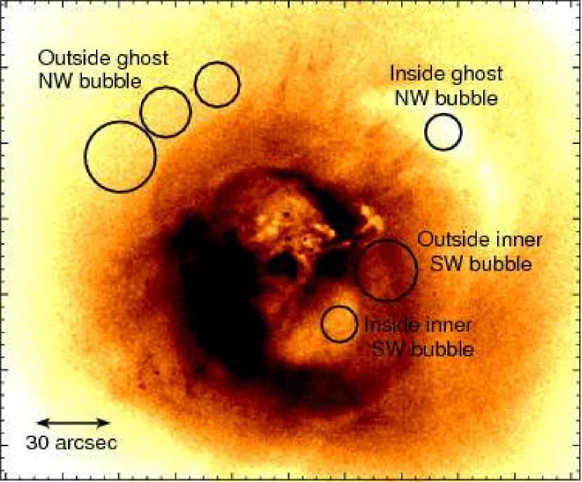
Figure 25: Regions used for examining the spectra inside and outside of the bubbles.

We examine the inner SW bubble and ghost NW bubbles using the regions shown in Fig. 25. Also indicated are the regions used for background. The inner NE bubble is obscured by the High Velocity System, so we do not consider that. The ghost S bubble has somewhat uncertain geometry. We try to place the regions away from any contamination by low temperature gas (though we have tried alternative regions with little effect), and the background regions at a similar radius to the bubbles. We assume the bubble regions are cylindrical in shape, with depths of 9.4 kpc and 13.4 kpc for the inner SW and ghost NW bubbles, respectively. We take the deprojected electron pressure of the surrounding thermal gas from the mean value of the sectors surrounding the bubbles in figure 19 of Sanders et al. (2004). This leads to values of 0.195 and $0.111\rm\thinspace keV\hbox{$\rm\thinspace cm^{-3}\,$}$ for the inner SW and ghost NW bubbles, respectively.

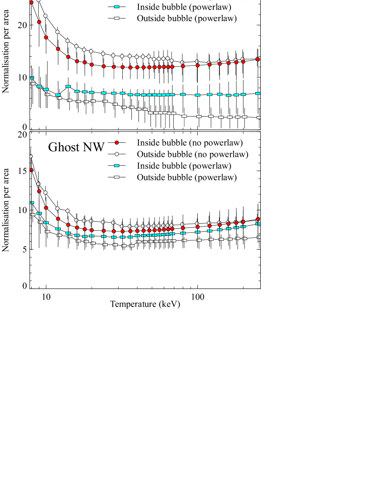
Figure 26: Hot thermal component normalisation per unit area (defined by the BACKSCAL header keyword) as a function of temperature inside the bubbles compared to outside. The results of including a $\Gamma=2$ powerlaw component are also shown.

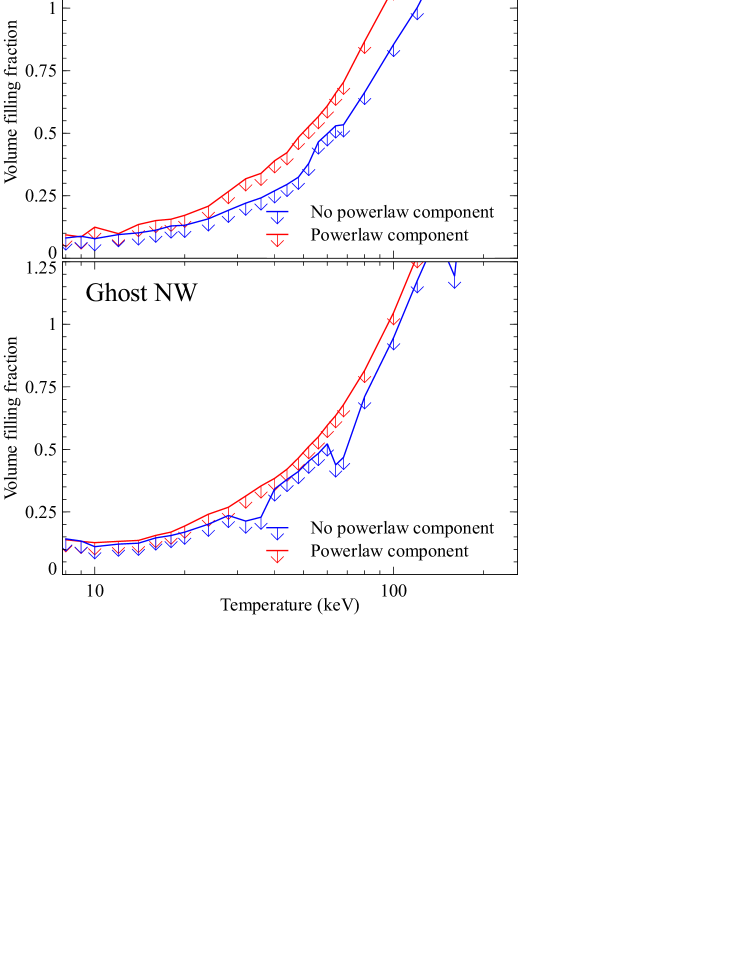
Figure 27: 2$\sigma$ upper limits to the volume filling fraction of the bubbles. Models including a $\Gamma=2$ powerlaw component are indicated.

For the two bubbles, including and not including the $\Gamma=2$ powerlaw component, we show the normalisation (emission measure) per unit area for the foreground and background regions in Fig. 26. We convert these values to upper limits on the volume-filling fraction in Fig. 27. We find that if there is volume-filling thermal gas within the bubbles, it must have a temperature of less than $\sim 100\rm\thinspace keV$ for either bubble.

9 Discussion

We have investigated several issues from the Chandra data of the Perseus cluster and now attempt to tie the interpretation of the various phenomena more closely together. In particular we try to understand the interplay between heating and cooling in the cluster core, and how energy is transported and distributed through the ICM.

9.1 Sound waves

Observations of Perseus and many other similar clusters show that jets feed relativistic plasma from around the massive central black hole into twin radio lobes. The power associated with this process is large and comparable to that required to balance radiative cooling within the regions of 50–100 kpc where the radiative cooling times is 3–5 Gyr (Rafferty et al., 2006; Dunn & Fabian, 2006). In the case of the Perseus cluster the jets are producing on average around $5\times 10^{44}-10^{45}\hbox{$\rm\thinspace erg\rm\thinspace s^{-1}\,$}$ in total, as estimated from the $P\mathrm{d}V$ work done over the 5-10 Myr age of the bubbles (Fabian et al., 2002b; Dunn & Fabian, 2004). These estimates depend on the filling factor of the bubbles by the relativistic plasma, which from the results given in Section 8 could well be unity. Therefore at least about 20–40 per cent of the bubble power goes into sound waves.

We expect the jets to provide power more or less continuously over the lifetime of the cluster core (several Gyr). This is supported by the high incidence of bubbles found in cluster cores that require heating (Dunn & Fabian, 2006) and by the train of ghost bubbles seen in our Perseus cluster data (Fabian et al., 2006). Note however, that there is probably much fluctuation in the jet power over short timescales (the radio source has weakened in strength over the past 40 yr), but variations over a cooling time of $10^{8}\rm\thinspace yr$ are probably less than an order of magnitude.

We now address the question of how the energy in the bubbling process, occurring on a timescale of 10 Myr, is fed into the bulk of the core and dissipated as heat which balances the cooling. The smooth cooling time profiles seen in cluster cores, and the peaked metal distributions argue for a relatively gentle, continuous (on timescales of $10^{7}-10^{8}\rm\thinspace yr$ or more) and distributed heat source. The inflation of the bubbles does $P\mathrm{d}V$ work on the surroundings and thus creates pressure waves – sound waves – which carry the energy outward in a roughly isotropic manner. We discovered ripples in surface brightness in the first 200 ks of the Perseus cluster data (Fabian et al., 2003a) which we interpreted sound waves and have extended the analysis of them here.

Fig. 5 shows that there is considerable power in these waves, around $2-3\times 10^{44}\hbox{$\rm\thinspace erg\rm\thinspace s^{-1}\,$}$ at radii of 30–70 kpc. It is similar to the level of heat required to offset radiative cooling within that region. The wave power drops with radius between 30 and 100 kpc indicating that the energy is being dissipated and confirming the idea that viscous dissipation of the sound waves is the distributed heat source. The dissipation length is comparable to that estimated on the basis of Spitzer-Braginski viscosity (Fabian et al., 2003a), although the process in the likely tangled magnetic, and cosmic-ray infused, plasma may be more complex and involve some form of bulk viscosity.

There is however a deficit of power shown by this analysis within 30 kpc. Although it could just be variability of the central power source (the jets), our results on the nonthermal component associated with the radio minihalo indicates that there is a significant nonthermal pressure from the cosmic rays there, comparable to the thermal pressure. This would quadruple (if the nonthermal wave pressure is the same as the thermal pressure in Equation 2) the predicted wave power in this region, bringing it into agreement with the region between 30 and 60 kpc and meaning that dissipation of sound waves can be the dominant heat source balancing radiative cooling.

The increase in power seen in Fig. 6 beyond 100 kpc can be explained as associated with the power $\sim 10^{8}\rm\thinspace yr$ ago being 2–3 times larger than present. This may fit in with the presence of the long Northern optical filament (Conselice et al., 2001), which if drawn out from the centre by a bubble (Hatch et al., 2006) must have been an exceptional bubble, possibly seen at 170 kpc north of the nucleus (Section 3.3). Also the ghost bubbles seen to the South in the X-ray pressure maps (Fabian et al., 2006) may be larger and so require more power than the present inner bubbles. If correct, the central source thus does vary by a factor of few on timescales of $10^{8}\rm\thinspace yr$. Deeper X-ray observations at larger radii than the current ones are needed to test this interesting possibility further.

We conclude the discussion of sound waves by noting that typical sound waves will be difficult to see in current data on other clusters. The X-ray surface brightness of the central 50 kpc of the Perseus cluster is more than twice that of another cluster. Large ripples, interpreted as weak shocks have been seen in the Virgo cluster (Forman et al., 2006) and possible outer ripples may occur in A 2199 and and 2A 0335+096 (Sanders & Fabian, 2006). These may just be the peaks in the distribution of sound waves in those clusters from the more exceptional power episodes of their central engines. Like tree rings or ice cores for the study of geological history, ripples in cluster cores offer the potential to track the past history of an AGN for more than $10^{8}\rm\thinspace yr$. Observations of a yet wider region are required to see where the ripples eventually die out.

9.2 The nonthermal component

We have reported on a hard X-ray component coincident with the radio minihalo (section 7). It is difficult to support a thermal origin for this emission in terms of a $\sim 16\rm\thinspace keV$ gas associated with the HVC. A simple energy argument against the thermal hypothesis is to note that the crossing time of the 200 kpc diameter inner core of the cluster at $3000\hbox{$\rm\thinspace km\rm\thinspace s^{-1}\,$}$ takes nearly $7\times 10^{7}\rm\thinspace yr$. The radiative cooling time of 16 keV gas with a plausible density of $10^{-2}\hbox{$\rm\thinspace cm^{-3}\,$}$ is $10^{10}\rm\thinspace yr$, so the shocked gas would radiate only 0.7 per cent of its energy. With the luminosity of this component at $5\times 10^{43}\hbox{$\rm\thinspace erg\rm\thinspace s^{-1}\,$}$ we obtain a total injected energy of $2\times 10^{61}\rm\thinspace erg$. This is the total kinetic energy of $2\times 10^{11}\hbox{$\rm\thinspace M_{\odot}$}$ moving at $3000\hbox{$\rm\thinspace km\rm\thinspace s^{-1}\,$}$. So an implausible large mass needs to be stripped from an apparently small galaxy in order to explain the hard component as due to shocking by the HVC.

The hard component is therefore most readily interpreted as inverse Compton emission from the minihalo. As discussed by Sanders et al. (2005) this means that it must be well out of equipartition for the electrons and magnetic field with the electrons dominating the nonthermal pressure (as also deduced for the radio lobes, Fabian et al. 2002b). It is possible that the radio bubbles leak a small fraction of their cosmic-ray electron content (and presumably protons or positrons for charge neutrality) into their surroundings. These accumulate, losing their energy principally through inverse Compton losses on the Cosmic Microwave Radiation. A half-power break in the power-law spectrum is then expected around 10 keV in the hard X-ray flux if this process has, as expected, been continuing for more than a Gyr. This matches what is inferred of the observed spectrum.

The presence of the nonthermal component increases the heating within the inner 30 kpc if $\delta P$ is raised proportionately, and also means that some direct collisional heating of gas is possible. Ruszkowski et al. (2007) have since investigated this idea in more detail.

9.3 The distribution of metals

The enhanced metallicity in the core of the Perseus cluster shows a spatial distribution which extends to the S along the axis of old bubbles, as expected if the bubbles push and drag the gas around (Roediger et al., 2007). What is particularly interesting here is evidence that the distribution is clumpy and also that the central drop is a real effect.

The clumpiness and especially the sharp edges of at least one clump (Fig. 13) likely require a magnetic field configured to prevent dispersal. The central metallicity drop is not easily explained as just due to some outer gas falling in to replace inner gas dragged out, since it has a significantly lower entropy. It could be accounted for if the metals are highly inhomogeneous on a small scale, with the higher metallicity gas which has the shorter cooling time cooling out (Morris & Fabian, 2003).

An interesting possibility raised by the high nonthermal pressure near the centre is that the gas is made buoyant by the cosmic rays (Chandran, 2004, 2005). In this picture the simple entropy inferred from just the gas temperature and density are insufficient to determine its behaviour. The gas cosmic-ray mixture becomes convectively unstable where the cosmic-ray pressure begins to drop steeply outward, leading to the gas overturning. The pressure drop is inferred to occur at about 30 kpc (Fig. 24) and is about the radius where the metallicity peaks (Fig. 9). Such a turnover of gas may happen sporadically when the cosmic-ray density has built up for some time.

9.4 The optical filaments

Finally we briefly discuss the H$\alpha$ filaments. These radiate most of their energy at Ly$\alpha$ (see Fabian et al. 1984 for an image) and are mostly composed of molecular gas at a few thousand down to 50 K (Hatch et al., 2005; Johnstone et al., 2007; Salomé et al., 2006). We have shown that they are surrounded and mixed with soft X-ray emitting plasma at 0.5–1 keV temperature. In section 6 we consider one filament in detail. The H$\alpha$ luminosity of its peak is about one per cent of the total measured by Heckman et al. (1989), so scaling the X-ray inferred mass cooling rate there of $0.06\hbox{$\hbox{$\rm\thinspace M_{\odot}$}\rm\thinspace yr^{-1}\,$}$ we obtain a total mass cooling rate into filaments of $5\hbox{$\hbox{$\rm\thinspace M_{\odot}$}\rm\thinspace yr^{-1}\,$}$.

This value assumes however that the X-ray emitting gas loses its energy solely by radiating X-rays. If in addition it loses energy by conduction, mixing or other means, with the cold gas in the filament and thereby powers the Ly$\alpha$ emission then we need to scale the above rate by a factor of 20 (the expected Ly$\alpha$/H$\alpha$ ratio for recombination) to obtain a total mass cooling rate of about $100\hbox{$\hbox{$\rm\thinspace M_{\odot}$}\rm\thinspace yr^{-1}\,$}$. This value agrees of course with that obtained by just taking the total H$\alpha$ luminosity and assuming it is obtained from the thermal energy of the hot gas. It is about one third of the total inferred mass cooling rate obtained if there is no heating. We note that radiation at other wavelengths such as O vi emission (Bregman et al., 2006) can increase this fraction.

This implies that a high non-radiative mass cooling rate is possible in the Perseus cluster. By extension, it suggest that this happens in most cool-core clusters (which generally also have optical filaments; see Crawford et al. 1999). It can account for part of the lack of cool X-ray emitting gas in such cluster cores (Fabian et al., 2002a).

A cooling rate of $100\hbox{$\hbox{$\rm\thinspace M_{\odot}$}\rm\thinspace yr^{-1}\,$}$ for 5 Gyr gives a total of $5\times 10^{11}\hbox{$\rm\thinspace M_{\odot}$}$ of cold gas. This is about 10 times more than is inferred from CO measurements (Salomé et al., 2006). Star formation is another possible sink. NGC 1275 has long been known to have an A-star spectrum and excess blue light. UV imaging of NGC 1275 by Smith et al. (1992) shows a lack of stars above $5\hbox{$\rm\thinspace M_{\odot}$}$, which means that any continuous star formation (which would have been only $20\hbox{$\hbox{$\rm\thinspace M_{\odot}$}\rm\thinspace yr^{-1}\,$}$) must have ended about 50 Myr ago. Burst models of star formation at rates up to many $100\hbox{$\hbox{$\rm\thinspace M_{\odot}$}\rm\thinspace yr^{-1}\,$}$ 100 Myr or so ago are consistent with the UV data (Smith et al., 1992). A picture in which gas accumulates through filaments and is then converted into stars sporadically on a 100 Myr timescale appears possible.

If however much of the power in the filaments is due to sources other than the hot gas, cosmic rays or kinetic motions for example, then the above star formation estimate is an upper limit.

9.5 Summary

We have quantified the properties of the X-ray surface brightness ripples found in the core of the Perseus cluster and, assuming that they are due to sound waves, have determined the power propagated as sound waves. The power found in this way is sufficient to balance radiative cooling within the inner 70 kpc, provided that it is dissipated as heat over this lengthscale. This provides the quasi-isotropic, relatively gentle, heating mechanism required to prevent a full cooling flow developing. Ultimately the power is derived from the jets emitted by the central black hole.

A hard X-ray component is confirmed and argued to be plausibly due to inverse Compton scattering by cosmic-ray electrons in the radio minihalo. The electrons may have leaked out of the radio lobes of 3C84 and now have a pressure comparable to the thermal pressure of the hot gas in the innermost 30 kpc. The lobes themselves appear to be devoid of any thermal gas unless its temperature is very high (50–100 keV). The cosmic-ray electrons are important in enhancing the heating and possibly also in changing the convective stability of the central 30 kpc.

The X-ray data provide insight on the history of the past 100 Myr of activity of the nucleus of NGC 1275. There are hints from the large ripples beyond 100 kpc, and from the the large Northern filament and the presence of many A stars, of a higher level of activity before that, a few 100 Myr ago. This can be tested by deep, high spatial resolution, observations of a wider region than covered out so far.

We infer that a close balance between heating and cooling is established in the core of the Perseus cluster over the past few 100 Myr. The average heating rate is, and has been, close to the radiative cooling rate, although there can be variations by a factor of a few on longer timescales. The primary energy source is the central black hole and jets; the energy is distributed by the sound waves generated by the inflation of the lobes. We suspect that this process is common to most cool core clusters and groups and is the mechanism by which heating of the cool core occurs. It will however be difficult to verify observationally in those other objects since the X-ray surface brightness is so much lower. Only the extreme peaks in the distribution of activity will generally be detectable.

Appendix A A Direct Spectral Deprojection Method

A.1 Problems with existing spectral deprojection methods

Results from fitting cluster data using the projct model in xspec can be misleading. projct is a model to fit spectra from several annuli simultaneously, to account for projection. There are one or more components per deprojected annulus, each with parameters (e.g. temperature, metallicity). The projected sum of the components along line of sights (with appropriate geometric factors) are fitted against each of the spectra simultaneously. Often the resulting deprojected profiles (e.g. temperature) oscillate between values separated by several times the uncertainties on the values. This oscillation can disappear if different sized annuli are used. Sometimes halving the annulus width can halve the oscillation period, indicating they are not physical changes on the sky.

The oscillation can be alleviated by fitting the shells sequentially from the outside, freezing the parameters of components in outer shells before fitting spectra from shells inside them (see e.g. Sanders et al. 2004). This helps to solve the issue where poorly modelled spectra near the centre can affect the results in outer annuli (The standard way to fit the data is simultaneous. All the spectra are used to calculate each point, even though interior shells and not projected in front of outer shells.) The difficulty with this method is that uncertainties calculated on parameters to the model are underestimated. They do not include the uncertainties on outer shells.

The outside-first fitting procedure does not fix every oscillating profile. Numerical experiments, when clusters are simulated and fit with projct (R. Johnstone, private communication), show that assuming the incorrect geometry when trying to account for projection does not produce oscillating profiles. Something which does create oscillating profiles are shells which contain more than one spectral component (e.g. several temperatures). It appears that projct tends to account for one of the components in one of the annulus fit results, and another in a different shell. By assuming that a spectral model is a good fit to the data, a very misleading result is produced. Other deprojection methods which assume a spectral model to do the deprojection will have similar issues.

A.2 Direct spectral deprojection

We describe here a method to create ‘deprojected spectra’, which appears to alleviate some of the issues found using projct. It is a model independent approach, assuming only spherical geometry (at present).

The routine takes spectra extracted from annuli in a sector, and their blank-sky background equivalents. From each of these foreground count rate spectra we subtract the respective blank sky background spectrum. Taking the outer spectrum, we assume that it was emitted from part of a spherical shell, and calculate the (count rate) spectrum per unit volume. This is then scaled by the volume projected onto the next innermost shell, and subtracted from the (count rate) spectrum from that annulus. After subtraction we calculate a spectrum per unit volume for the next innermost shell. We move inwards shell-by-shell, subtracting from each the calculated contributions from outer shells. This yields a set of deprojected spectra which are then directly fitted by spectral models.

To calculate the uncertainties in the count rates in the spectral channels in each spectrum we used a Monte Carlo technique. Firstly each of the input foreground and background spectra are binned using the same spectral binning, using a large number of counts per spectra channel (we used 100 in this work) so that Gaussian errors can be assumed in each spectral bin. We repeat the deprojection process 5000 times, creating new input foreground and background spectra by simulating spectra drawn from Gaussian distributions based on the initial spectra and their uncertainties. The output spectra are the median output spectra from this process, and the 15.85 and 84.15 percentile spectra were used to calculate the 1$\sigma$ errors on the count rates in each channel.

This technique assumes that the response of the detector does not change significantly over the detector. This is the case for the ACIS-S3 detector on Chandra used here. It also assumes that the effective area does not change significantly, as we do not account for the variation of the ancillary response. This could be incorporated into this method, but we have not implemented this yet.

References

- Allen et al. (2001) Allen S. W., Schmidt R. W., Fabian A. C., 2001, MNRAS, 328, L37
- Anders & Grevesse (1989) Anders E., Grevesse N., 1989, Geochim. Cosmochim. Acta, 53, 197
- Arnaud (1996) Arnaud K. A., 1996, in Jacoby G. H., Barnes J., ed, ASP Conf. Ser. 101: Astronomical Data Analysis Software and Systems V, p. 17
- Balucinska-Church & McCammon (1992) Balucinska-Church M., McCammon D., 1992, ApJ, 400, 699
- Böhringer & Fabian (1989) Böhringer H., Fabian A. C., 1989, MNRAS, 237, 1147
- Böhringer et al. (1993) Böhringer H., Voges W., Fabian A. C., Edge A. C., Neumann D. M., 1993, MNRAS, 264, L25
- Bregman et al. (2006) Bregman J. N., Fabian A. C., Miller E. D., Irwin J. A., 2006, ApJ, 642, 746
- Brüggen et al. (2007) Brüggen M., Heinz S., Roediger E., Ruszkowski M., Simionescu A., 2007, ArXiv e-prints, arXiv:0706.1869
- Cash (1979) Cash W., 1979, ApJ, 228, 939
- Chandran (2004) Chandran B. D. G., 2004, ApJ, 616, 169
- Chandran (2005) Chandran B. D. G., 2005, ApJ, 632, 809
- Churazov et al. (2000) Churazov E., Forman W., Jones C., Böhringer H., 2000, A&A, 356, 788
- Churazov et al. (2003) Churazov E., Forman W., Jones C., Böhringer H., 2003, ApJ, 590, 225
- Conselice et al. (2001) Conselice C. J., Gallagher J. S., III, Wyse R. F. G., 2001, AJ, 122, 2281
- Crawford et al. (1999) Crawford C. S., Allen S. W., Ebeling H., Edge A. C., Fabian A. C., 1999, MNRAS, 306, 857
- Dunn & Fabian (2004) Dunn R. J. H., Fabian A. C., 2004, MNRAS, 355, 862
- Dunn & Fabian (2006) Dunn R. J. H., Fabian A. C., 2006, MNRAS, 373, 959
- Dunn et al. (2006) Dunn R. J. H., Fabian A. C., Sanders J. S., 2006, MNRAS, 366, 758
- Erlund et al. (2006) Erlund M. C., Fabian A. C., Blundell K. M., Celotti A., Crawford C. S., 2006, MNRAS, 371, 29
- Fabian et al. (2002a) Fabian A. C., Allen S. W., Crawford C. S., Johnstone R. M., Morris R. G., Sanders J. S., Schmidt R. W., 2002a, MNRAS, 332, L50
- Fabian et al. (2002b) Fabian A. C., Celotti A., Blundell K. M., Kassim N. E., Perley R. A., 2002b, MNRAS, 331, 369
- Fabian et al. (1984) Fabian A. C., Nulsen P. E. J., Arnaud K. A., 1984, MNRAS, 208, 179
- Fabian et al. (2005) Fabian A. C., Reynolds C. S., Taylor G. B., Dunn R. J. H., 2005, MNRAS, 363, 891
- Fabian et al. (2003a) Fabian A. C., Sanders J. S., Allen S. W., Crawford C. S., Iwasawa K., Johnstone R. M., Schmidt R. W., Taylor G. B., 2003a, MNRAS, 344, L43
- Fabian et al. (2003b) Fabian A. C., Sanders J. S., Crawford C. S., Conselice C. J., Gallagher J. S., Wyse R. F. G., 2003b, MNRAS, 344, L48
- Fabian et al. (2000) Fabian A. C. et al., 2000, MNRAS, 318, L65
- Fabian et al. (2006) Fabian A. C., Sanders J. S., Taylor G. B., Allen S. W., Crawford C. S., Johnstone R. M., Iwasawa K., 2006, MNRAS, 366, 417
- Forman et al. (2006) Forman W. et al., 2006, ArXiv preprint astro-ph/0604583
- Gillmon et al. (2004) Gillmon K., Sanders J. S., Fabian A. C., 2004, MNRAS, 348, 159
- Hatch et al. (2005) Hatch N. A., Crawford C. S., Fabian A. C., Johnstone R. M., 2005, MNRAS, 358, 765
- Hatch et al. (2006) Hatch N. A., Crawford C. S., Johnstone R. M., Fabian A. C., 2006, MNRAS, 367, 433
- Heckman et al. (1989) Heckman T. M., Baum S. A., van Breugel W. J. M., McCarthy P., 1989, ApJ, 338, 48
- Johnstone et al. (2007) Johnstone R., Hatch N., Ferland G., Fabian A., Crawford C., Wilman R., 2007, ArXiv preprint astro-ph/0702431
- Kaastra (1992) Kaastra J. S., 1992, An X-ray spectral code for optically thin plasmas, Technical report, SRON, updated version 2.0
- Landau & Lifshitz (1959) Landau L. D., Lifshitz E. M., 1959, Fluid mechanics. Course of theoretical physics, Oxford: Pergamon Press, 1959
- Liedahl et al. (1995) Liedahl D. A., Osterheld A. L., Goldstein W. H., 1995, ApJ, 438, L115
- Lynds (1970) Lynds R., 1970, ApJ, 159, L151
- McNamara et al. (2005) McNamara B. R., Nulsen P. E. J., Wise M. W., Rafferty D. A., Carilli C., Sarazin C. L., Blanton E. L., 2005, Nat, 433, 45
- Mewe et al. (1985) Mewe R., Gronenschild E. H. B. M., van den Oord G. H. J., 1985, A&AS, 62, 197
- Mewe et al. (1986) Mewe R., Lemen J. R., van den Oord G. H. J., 1986, A&AS, 65, 511
- Minkowski (1957) Minkowski R., 1957, in van de Hulst H. C., ed, IAU Symp. 4: Radio astronomy, p. 107
- Morris & Fabian (2003) Morris R. G., Fabian A. C., 2003, MNRAS, 338, 824
- Nevalainen et al. (2004) Nevalainen J., Oosterbroek T., Bonamente M., Colafrancesco S., 2004, ApJ, 608, 166
- Nipoti & Binney (2004) Nipoti C., Binney J., 2004, MNRAS, 349, 1509
- Nulsen et al. (2005a) Nulsen P. E. J., Hambrick D. C., McNamara B. R., Rafferty D., Birzan L., Wise M. W., David L. P., 2005a, ApJ, 625, L9
- Nulsen et al. (2005b) Nulsen P. E. J., McNamara B. R., Wise M. W., David L. P., 2005b, ApJ, 628, 629
- Pedlar et al. (1990) Pedlar A., Ghataure H. S., Davies R. D., Harrison B. A., Perley R., Crane P. C., Unger S. W., 1990, MNRAS, 246, 477
- Peterson & Fabian (2006) Peterson J. R., Fabian A. C., 2006, Phys. Rep., 427, 1
- Peterson et al. (2003) Peterson J. R., Kahn S. M., Paerels F. B. S., Kaastra J. S., Tamura T., Bleeker J. A. M., Ferrigno C., Jernigan J. G., 2003, ApJ, 590, 207
- Primini et al. (1981) Primini F. A. et al., 1981, ApJ, 243, L13
- Rafferty et al. (2006) Rafferty D. A., McNamara B. R., Nulsen P. E. J., Wise M. W., 2006, ApJ, 652, 216
- Rebusco et al. (2005) Rebusco P., Churazov E., Böhringer H., Forman W., 2005, MNRAS, 359, 1041
- Roediger et al. (2007) Roediger E., Brüggen M., Rebusco P., Böhringer H., Churazov E., 2007, MNRAS, 375, 15
- Ruszkowski et al. (2004) Ruszkowski M., Brüggen M., Begelman M. C., 2004, ApJ, 611, 158
- Ruszkowski et al. (2007) Ruszkowski M., Ensslin T. A., Bruggen M., Begelman M. C., Churazov E., 2007, ArXiv e-prints, arXiv:0705.3235
- Salomé et al. (2006) Salomé P. et al., 2006, A&A, 454, 437
- Sanders (2006) Sanders J. S., 2006, MNRAS, 371, 829
- Sanders & Fabian (2006) Sanders J. S., Fabian A. C., 2006, MNRAS, 371, L65
- Sanders et al. (2004) Sanders J. S., Fabian A. C., Allen S. W., Schmidt R. W., 2004, MNRAS, 349, 952
- Sanders et al. (2005) Sanders J. S., Fabian A. C., Dunn R. J. H., 2005, MNRAS, 360, 133
- Schmidt et al. (2002) Schmidt R. W., Fabian A. C., Sanders J. S., 2002, MNRAS, 337, 71
- Sijacki & Springel (2006) Sijacki D., Springel V., 2006, MNRAS, 366, 397
- Sijbring (1993) Sijbring D., 1993, Ph.D. thesis, Groningen Univ.
- Smith et al. (1992) Smith E. P. et al., 1992, ApJ, 395, L49
- Smith et al. (2001) Smith R. K., Brickhouse N. S., Liedahl D. A., Raymond J. C., 2001, ApJ, 556, L91
- Spitzer (1962) Spitzer L., 1962, Physics of Fully Ionized Gases. Physics of Fully Ionized Gases, New York: Interscience (2nd edition), 1962